Article

Using a Statistical Crop Model to Predict Maize Yield by the End-Of-Century for the Azuero Region in Panama

by
Marlemys M. Martínez
1,
Tosiyuki Nakaegawa
2,
Reinhardt Pinzón
3,4,
Shoji Kusunoki
2,5,
Román Gordón
6 and
Javier E. Sanchez-Galan
4,7,*
1
Facultad de Ciencias y Tecnología, Universidad Tecnológica de Panamá (UTP), P.O. Box 0819-07289 El Dorado, Panama
2
Meteorological Research Institute, Tsukuba 305-0052, Ibaraki, Japan
3
Centro de Investigaciones Hidráulicas e Hidrotécnicas, Universidad Tecnológica de Panamá (UTP), P.O. Box 0819-07289 El Dorado, Panama
4
Centro de Estudios Multidisciplinarios de Ingeniería Ciencias y Tecnología (CEMCIT-AIP), P.O. Box 0819-07289 El Dorado, Panama
5
Faculty of Societal Safety Sciences, Kansai University, Takatsuki-shi 569-1098, Osaka, Japan
6
Instituto de Investigación Agropecuaria de Panamá (IDIAP), Estafeta de Los Santos, 0739 Los Santos, Panama
7
Facultad de Ingenieria de Sistemas Computacionales, Universidad Tecnológica de Panamá (UTP), P.O. Box 0819-07289 El Dorado, Panama
*
Author to whom correspondence should be addressed.
Atmosphere 2020, 11(10), 1097; https://doi.org/10.3390/atmos11101097
Submission received: 10 September 2020 / Revised: 4 October 2020 / Accepted: 8 October 2020 / Published: 14 October 2020
(This article belongs to the Special Issue Climate Change and Agrometeorological Time Series)

Abstract

:
In this article, we evaluate the impact of temperature and precipitation at the end of the 21st century (2075–2099) on the yield of maize in the Azuero Region in Panama. Using projected data from an atmospheric climate model, MRI-ACGM 3.2S, the study variables are related to maize yield (t ha 1 ) under four different sea surface Temperature (SST) Ensembles (C0, C1, C2, and C3) and in three different planting dates (21 August, 23 September, and 23 October). In terms climate, results confirm the increase in temperatures and precipitation intensity that has been projected for the region at the end of the century. Moreover, differences are found in the average precipitation patterns of each SST-ensemble, which leads to difference in maize yield. SST-Ensembles C0, C1, and C3 predict a doubling of the yield observed from baseline period (1990–2003), while in C1, the yield is reduced around 5%. Yield doubling is attributed to the increase in rainfall, while yield decrease is related to the selection of a later planting date, which is indistinct to the SST-ensembles used for the calculation. Moreover, lower yields are related to years in which El Niño Southerm Oscilation (ENSO) are projected to occur at the end of century. The results are important as they provide a mitigation strategy for maize producers under rainfed model on the Azuero region, which is responsible for over 95% of the production of the country.

1. Introduction

The biophysical effect of changing climate patterns on agriculture and crop management has been largely studied [1,2]. Moreover, the impact of this change is known to be higher in developing countries and small farmers relegated to subsistence rainfed agriculture (no irrigation) [3]. Therefore, it is imperative for countries to study the changes in their yield values in actual climates, and simulate their yields in future climates [4]. In fact, this process often is done via biophysical models, agro-ecological models, statistical analysis models, and global gridded crop models. These models are done to provide worldwide estimates, usually for selected crops (high food energy cereals) such as maize, wheat, rice, and soybean [4,5], and often are studied in relation to food security [6]. However, there are also studies carried out on crops of specific economical interest in a country, or those used as foodstuffs, such as sugarcane or others [7]. A comprehensive review of the effects of climate change in agricultural crops is provided in [8].
Some studies have been geared toward the projection of maize in countries or regions, for instance, in the case of the Latin American region, a seminal 2003 article by Jones and Thornton [9] is often used as an example. In this article, the authors focuses on the impact that climate change will have on maize for Africa and Latin America, country by country up to 2055, using the Crop Estimation through Resource and Environment Synthesis crop model (CERES)-Maize models. The authors project an overall 10% decrease in maize yield in 2055, but suggest that this be counteracted with technological interventions and selective plant breeding. For the case of maize yield in Panama, Jones and Thornton [9] calculate a loss of 238 kg ha 1 which represents a loss of more than 14,000 tonnes in 2055. In the work by Ruane et al. [
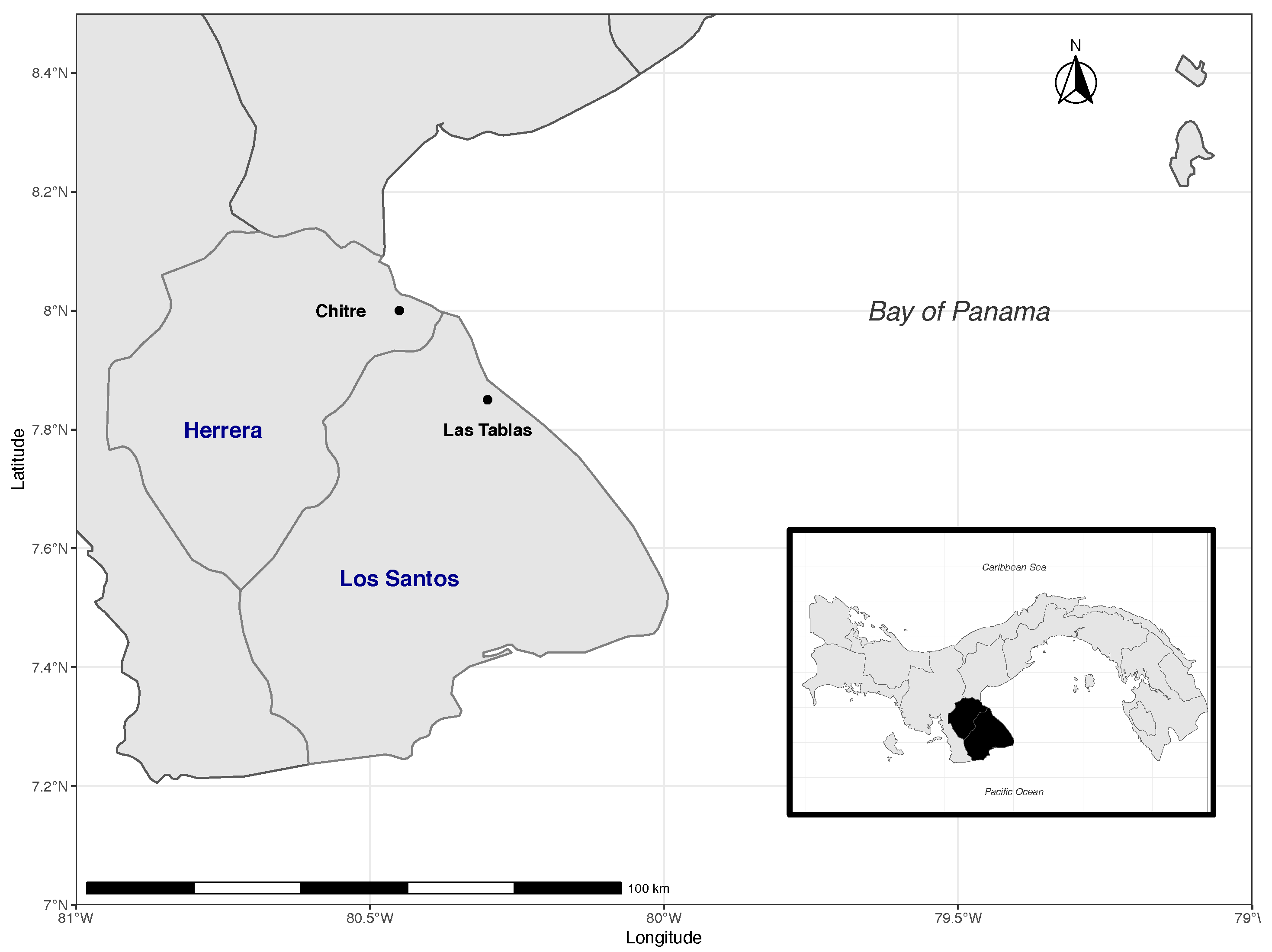
10], a clearer picture is presented about Panama and the production of maize. The authors focus on Los Santos and investigate the impact on maize yield in three distinct time periods: near-term (2005–2034), mid-century (2040–2069), and end-of-century (2070–2099) using an ensemble of 16 GCM models and the CERES-Maize model in two different scenarios, one with high emissions A2 (comparable forcing as RCP8.5) and low emission B1 (comparable to RCP 4.5). The resulting yields are as follows (for A2 and B1, respectively), decrease of 0.5% and 0.1% for near-term, increase of 2.4% and decrease of 0.8% for mid-century, and increase of 4.5% and 1.5% for end-of-century.
Besides these process-based models, other developments are based on statistical crop yield models, often called empirical models. In terms of their output, both models are comparable having strong overlap in their results [11,12,13]. The first type of model often include the effects of CO 2 which can be related to warming, while in statistical models this is not accounted for [11]. Kogo et al. [14] states that while simulation and process-based models need to be validated, a regression model is adjusted from real agronomic yields, thus reflecting the true phenomenon. In Holzkämper et al. [15], the effects of temperature and precipitation has been assessed with a statistical crop model for maize. In Holzkämper et al. [16], the analysis is extended to include both process-based and statistical crop models for the determination of climate impact on maize. Specifically in regards to statistical methods, Shi et al. highlights the issues existing in the crop yield sensitivity to climate change using statistical models, which include defining the extent of spatial and temporal scales, trend removal, and removing co-linearity in models. Some of this issues are also discussed in [17].
The case of the future climate in The Republic of Panama has been addressed by many researchers and with different models. However, a considerable number of studies have focused in precipitation at the End-of-Century data using the MRI-AGCM model [18,19,20,21]. Most of these studies indicate that in the future, precipitation will increase in the central and eastern parts of Panama from May to November, corresponding to the rainy season. The increase in precipitation in most regions can be attributed to the increased transport of water vapor originating in the Caribbean Sea, which converges on Panama.
Compared to the amount of work dedicated to predictive climate studies for Panama, less work has been done regarding the implications of these future climate changes. Early work by Espinosa et al. [22] assessed the impact of climate change impacts on the water resources of Panama for three regions in La Villa (Los Santos Province), Chiriquí, and Chagres river basins. In [23], the climate change is assessed for agricultural development for the highlands of Western Panama in Chiriquí Province. More interestingly, Garcia et al. [24] focused on climate anomalies found on the projections for La Villa River Basin for the years 2050 and 2070 using data from the WorldClim Meteorological Database.
In fact, aside from Ruane’s efforts using a process-based model for maize in the Azuero Region, little research has been carried out to evaluate climatic scenarios and relate their implications on crop yields. In response to this reality, the objectives of this work are as follows. (1) Explore the meteorological predictions data set provided by the MRI-ACGM model. (2) Study the projected precipitation and temperature for the RCP8.5 scenarios for four different Sea Surface Temperature ensembles. (3) Explore the impact of precipitation and temperature in the Azuero Region using a statistical crop model and study its implications for maize production in different planting dates. (4) Provide bias-corrected estimates for key meteorological variables for further use.

2. Materials and Methods

2.1. Location of the Study

Maize cultivation in Panama is concentrated in the eastern portion of the Azuero Peninsula that extends into the Pacific from the south of the country [25]. The Azuero Region has limits to the north with the provinces of Coclé and Veraguas, to the south with the Pacific Ocean, to the east with the Gulf of Montijo, and to the east with the Gulf of Panama. In the same area, the provinces of Herrera, Los Santos, and the southeastern part of the province of Veraguas are located (as shown in Figure 1).
The tropical climate of the country is affected by the seasonal migration of the inter-tropical convergence zone (ITCZ) where two maize growing seasons are established: “first plantation” and “second plantation”. In addition, the particular case of the Azuero Region with respect to its location near sea level (for instance the town of Los Santos is at an altitude of 16 m) and a coastal climate consistent with the scales of the GCMs, which allows working with future C O 2 emissions scenarios [10].

2.2. Meteorological Data Source

The Empresa de Transmisión Eléctrica or ETESA is the entity in charge of the hydro-meteorological functions in Panama and has a National hydro-meteorological Network of more than 215 stations [26]. The data used for this study are observations from 1st January 1965 to 31st December 2017 from the meteorological station No. 128-001, located in the town of Los Santos, Los Santos province, one of the more longstanding stations in the region The global coordinates of the measurement area are longitude 7 56 27 and latitude 80 25 03 . It is a type A Conventional climate station (mechanical), attended daily by meteorological observers trained to make readings of the different instruments that measure rainfall, temperature and relative humidity of the air, and evaporation. According to historical data, the annual average rainfall is 1066.4 mm and the average annual temperature is 27.8 C.
At the country-wide level there are three regions in terms of rainfall regime: Pacific Region, Central Region, and Atlantic Region. We highlight the Pacific Region where the Azuero Region is located and is characterized by abundant rains of moderate to heavy intensity, accompanied by electrical activity that occurs especially in the afternoon. The rainy season starts firmly in the month of May and lasts until November, with the months of September and October having the highest rainfall. However, a dry period known as Veranillo frequently occurs, associated with the absence of precipitation, between late June, July and August [10,27].

2.3. Projected Metereological Data

Among the many models that make part of the 5th phase of CMIP (CMIP5), the MRI-AGCM model is of interest for this work [28] because of high horizontal resolutions and high performance in present climate simulations. This model was jointly developed by the Japan Meteorological Agency (JMA) and the Meteorological Research Institute of Japan (MRI). The last generation of this model is MRI-ACGM 3.2 [29]. The 20 km horizontal resolution used in this study is one of the finest horizontal grid spacing in the latest 6th phase of CMIP (CMIP6) as well as in CMIP5. This model is AGCM without the ocean component in order to represent present climate without almost no biases in sea surface temperature (SSTs) by prescribing observed SSTs and to properly simulate extreme events such as tropical cyclones which are composed of small-scale convection activities. This model, however, inherently has no atmosphere–ocean interactions, which may slightly affect the future climate projections, but has one of the best representations of present climates in CMIP5 models. This model has been used for the projections of rain [21,30] and surface air temperature in South America [21,30] or other hydroclimatic variables in Panama [20], Central America, and the Caribbean [31].
The projected data contained projections for the Central American region (including Panama) at 60 km and 20 km of grid cell resolution. The model had projected values for two variables—precipitation and temperature—under the RCP8.5 (Representative Concentration Pathway) trajectory. This trajectory describes how emissions continue to rise throughout the 21st century, with radiative forcing values of +8.5 W / m 2 of C O 2 in the year 2100. This increase is measured in relation to the registered pre-industrial values. This is one of the trajectories and scenarios described by the Intergovernmental Panel on Climate Change (IPCC AR5) [32].
Present time data (SPA 8.5) were obtained from the Sea Surface Temperature (SST) multimodel set mean pattern calculated from future projections of the 18 CMIP3 models for the 1979–2003 period. Future time data (SFA 8.5) is composed of four different projections of future SSTs for the 2075–2099 period. Each projection encompasses a particular spatial SST anomaly pattern. The four projections can be described as follows: the C0 SST-ensemble projection, which is a multimodel ensemble mean SST computed from future projections by the 18 CMIP3 models, and the C1 SST-ensemble, which results as the first cluster identified in a clustering analysis of the 18 CMIP3 models. The C1 projection is known to have less spatial variation in warming over the tropics in relation to the other clusters and also that it shows that the warming in the southern hemisphere is greater than in the northern hemisphere. The C2 projection is similar to the CMIP3 ensemble average, characterized by a greater warming in the Indian Ocean. Finally, C3 has the largest spatial variation among all SST, and is distinguished by visible warming near Japan (western Pacific and subtropical central Pacific). For a detailed presentation of the methods for the creation of the projections the reader is advised to check Murakami et al. [33,34].
Among the GCMs participating in CMIP5, the MRI-AGCM is the one with the highest horizontal resolutions. I has a resolution of 20 km. The other CMIP5 models have typically horizontal resolution of 100 to 200 km grid spacing or 10,000 to 40,000 km 2 . The whole Azuero peninsula has an area of 8000 km 2 (with a length of 100 km and a width of 90 km). In contrast to the Azuero Region, we only consider the eastern part of this peninsula in this study, which has linear measurements of ~100 km. Therefore, CMIP5 models have problems and cannot resolve the Azuero Region, but MRI-AGCM can do a good job in the present climate simulation in Panama as described in [21]. Due to the limited computer resources, 25-year simulations in both the present and future climates are available at the end-of-century. It is noteworthy that 20 km simulations consume about 10 3 computer resources for 200 km simulations. Therefore, a 25-year time-sliced period was chosen for this study, instead of a sequential simulation for the whole period.
Moreover, RCP8.5 was selected because of having the highest radiative forcing among the RCPs. Instead of projecting other RCP scenarios, the MRI-AGCM model explores four different spatial uncertainties in future changes in SST with 20 km grid spacing. Based on the premise that future changes in climates especially precipitation and surface air temperatures under the three other RCPs are in range from the present climate to the climate under the RCP8.5 and as such can be interpolated.

2.4. Historical Maize Production in Panama and Azuero

In Panama, more than 487,000 tons of maize are consumed per year, of which 96,600 (around 20%) are produced domestically and the rest are imported. Most of the commercial maize (around 88%) is used for animal feed, and the rest is for human consumption. In the Azuero region, the planted area has been on average of 18,000 hectares in the last ten seasons [35]. In fact, it has been calculated that over 97% of the national production is produced in the Azuero Region [27]. In terms of yield, the average tonnage per hectare (t ha 1 ) area calculated for the region from 1990 to 2017 is 3.9 t ha 1 . A graph detailing the yield per year is shown in Figure 2.
It is important to notice that in this graph that the year 1997, which is accounted as one of the hardest hitting El Niño–Southern Oscillation (ENSO) in the Region, a proactive mitigation work was put in place. The planting plots was mostly carried out on the southernmost part of the Azuero Region, where in general there is more water availability, thus not affecting the total yield for the year. However, the total sown and harvested area were considerably lower that previous years. A different scenario happened during the 2015 ENSO event. Mitigation measures were not put in place and a significant reduction of the total yield was tabulated for the 2015, as it can be seen in Figure 2, when comparing the 2014, 2015, and 2016 yields per hectare.

Maize Yield Model

A long-term experiment that began in 2015 at the El Ejido Experimental Station of IDIAP has been set up to evaluate two hybrid materials: one susceptible (Pioneer 30F-35) and the other tolerant (P-4226) to water deficiencies. Seeds are place into plots in dry land (depending on the rainfall of the locality) and with supplementary drip irrigation to meet the water demands of the crop. Three sowings are carried out per year to subject the crop to different rainfall regimes and other climatic variables such as temperature, relative humidity, VPD, solar radiation, and UV in the different periods of crop development.
To further understand the grain yield a regression model was developed for the 30F-35 variety and two of climatic variables were considered, precipitation and temperature. Correlating the yield of a crop to an unique climatic variable or to single planting day is difficult. This is because yield is highly influenced by the weather throughout its development. To solve this situation, the growth stages of the crop that are most affected by water deficiencies are taken into account.
One way to do this is to adjust the days after planting according to the development of the crop. For Panama, in Saéz et al. [37], the authors correlated the yield with the average of the different climatic variables in each growth stage. According to Denmead and Shaw [38] and McWilliams et al. [39], the stages can be divided as follows.
  • The first stage goes from germination to V9 (0 to 30 days after planting – DAP); in this stage, the hydric deficiency affects very little the grain yield and there are no losses in the yield if hydric deficiencies appear.
  • The second stage begins in V10 until VT (31 to 50 DAP), in this period several components of the yield are defined, such as the number of rows and the number of grain per row of the ears. A deficiency in this stage can cause up to a 25% reduction in performance potential.
  • The third stage begins in R1 and ends in R3 (51 to 80 DAP); this is the most critical stage of the crop [40], it is the stage where the plant has the highest water consumption [41], a water deficiency in the crop can reduce the yield up to 50% of its potential.
  • The fourth and last stage comprises from R4 to R6, and in this stage there may be a 25% reduction in the presence of water deficiencies in the development of the crop.
Finally, the yield was correlated with the climatic conditions in each of these stages with a regression model. The regression was fitted with observed data from the Azuero region for the 2015, 2016, and 2017 harvest years, under rainfed conditions. The resulting model achieved a R 2 of 0.96 with all the parameters of the equation being significant (p < 0.10). The resulting model and its coefficients are expressed in the Equation (1). Further details of the fitting of the model are described in Table A1.
Y i e l d = 0.028 × P R E 3 2.078 × T E M P 3 + 0.045 × P R E 4 + 2.109 × T E M P 4
where Yield is the grain yield in t ha 1 , P R E 3 represents the accumulated rainfall between 51 and 80 DAP, T E M P 3 represents the average temperature between 51 and 80 DAP, P R E 4 represents accumulated rainfall between 81 and 100 DAP, and T E M P 4 represents the average temperature between 81 and 100 DAP. It is important to notice that the sub-indexes 3 and 4 are just a way to refer to third and fourth stages of the crop growth. A validation of the model is described in detail in the Appendix A, with Table A2, showing the residuals of the model in two subsequent periods 2018 and 2019.
It is important to explain that the regression model presented has a way to account for independent climatic effects. In fact, to isolated the effect of rain in crop yield, three different planting dates (21 August, 23 September, 10 October) are used. These dates are important as they are correlated to the precipitation and overall water availability of the Azuero Region. Rainfall in the Azuero region begins at the end of April and increases until September, and decreases in November until stopping in December. These dates are important from the plating perspective and further the delay in planting the greater the impact on the yield [25].

2.5. Determining the Impact of Future Climate in Maize Yield at the End-of-century

For determining the impact of future climate in Maize Yield for Azuero, first the accumulated rainfall and the average temperature for the 2075–2099 period were extracted in correspondence to the normal planting intensive months in the Azuero region (August to December) for both C0 and C1 SST-ensembles.
The analysis consisted of comparing the average maize yield observed and projected for present time (Figure 2), to the calculated yield using Equation (1) with projected estimates (C0, C1, C2, and C3 ensembles) for precipitation and temperature. Moreover, a comparison between plantation dates was made, with 100 DAP happening in an earlier date (21 August), a middle date (23 September), and later date (10 October), reflecting the extremes of planting dates that have been observed in the Azuero region [25,27].
A simple delta-change correction Equation (2) was proposed to adjust the yield values predicted by the regression model in present time data (SFA):
Y c = Y p p × Y ¯ h i s t Y ¯ p p
where Y c is the corrected yield, Y h i s t is the average historical yield for the period, and Y p p the average yield projected by the model.
For future time yield, a modified version of Equation (2) is used. It was modified to be used as estimates for the end-of-century calculations, in the similar way that Araya et al. used it in [42]. The modified equation is shown in (3):
Y f c = Y f p × Y ¯ p p Y ¯ f p
where Y f c is the corrected yield, Y p p is the present time average yield, and Y f p the average future yield projected by the model at the end of century.

2.6. Bias Correction for Projections

Climate modeling is far from perfect and it is known that models tend to overestimate the projected values. Moreover, most GCMs do not consider regional information in their resolutions, and therefore information is lost on topographic variability and related atmospheric processes, causing errors and uncertainties. Bias correction is a postprocessing technique useful to provide a better fit to the output values of model that can be biased due to the uncertainty in parameterization of unsolved or unaccounted processes [43]. Various methods have been developed to make these corrections, such as Bias correction [44,45], Delta Change method, Change Factor, Linear scaling, Variance Scaling, Power Transformation, and Quantile mapping [46,47]. Among these correction methods listed, the Delta Method is often used to correct the variables of extreme temperatures and rainfall was of interest. Therefore, in this work the Delta Method was selected to correct for errors in projection estimates of average maximum and minimum temperature and daily precipitation estimates [31].
The equations used to correct the temperature (T) (Equation (4)) and precipitation (P) (Equation (5)) are listed below,
T f c = T h i s t + ( T ¯ f p T ¯ p p )
P f c = P h i s t × P ¯ f p P ¯ p p
where T f c and P f c are the corrected future estimates for temperature and precipitation, f p is the future time projected data (SFA), p p is present time projected data (SFA), and h i s t is the historical observed that data for each of the variables. These bias correction equations were used for both SST-ensembles C0 and C1 to estimate corrected temperature and corrected precipitation values.

3. Results and Discussion

3.1. Assessment of the Projected Data

For the extraction of the projected data, a subroutine was defined in Grid Analysis and Display System (GrADS). Latitude and longitude were varied to obtain data at the country level and then adjusted to further analyze the Azuero Region for both temperature and precipitation. For each variable daily projections were grouped in monthly files and further analyzed.
Furthermore, a comparison was made between the four different SST-ensembles schemes for the variables precipitation (Figure 3A) and average daily temperature (Figure 3B) and both extremes, minimum (Figure 3C) and maximum temperatures (Figure 3D), for all SST-ensembles.
According to Figure 3A, plot for C0 shows the typical heat wave of the Azuero Region. Interestingly, it shows the same pattern of Veranillo, with a decrease in precipitation in the month of June. In contrast, for projections under C1 a big change in precipitation months appears. The peak rainy season, usually perceived in October is shown to happen in June. This shift is very important since, the maize planting period usually is centered around this peak in Azuero and historically, the average for the region in the months August–December is around 635mm. On the other hand, projections for C2 follows a shifted but almost normal pattern with highest rainfall would be June–August. This implies that SST-Ensembles C1 and C2 project significant variations in Azuero precipitation at the end of the century. It can also be suggested that C0 will reflect the present time climate for the localities to the northern part of the Azuero region, while C1, C2, and C3 will reflect present climates that now occur on localities on the southern portion of Azuero region. This with respect to data observations in years prior to the current [25].
In regards to monthly temperatures for the Azuero region at the end-of-century, Figure 3B shows that the four SST-ensembles project temperatures above the annual average temperature 27.8 C [26], but remain between the average temperature for the Azuero Region (28 C and 34 C).
Figure 3C shows the monthly averages of extreme minimum temperature. Figure 3D shows the monthly averages of extreme maximum temperature. The minimum temperatures are projected to be between 28 C and 30 C. While the maximum temperatures are projected to be between 29 C and 32 C. According to the data from the work in [21], values are observed for the minimum temperatures (14.4 C and 18.3 C) and maximum (35.4 C and 38.4 C) in the Azuero region from historical data. When comparing historical values versus projected values, we can affirm that the model tends to overestimate the minimum temperature and underestimate the maximum temperature.

3.2. Crop Yield

Using the model in Equation (1) and the projected data shown in Figure 3, initial yield estimates for present time data (SPA) for Azuero region were calculated. A comparison of the historical yields in the 1990–2003 (average of 3.5 t ha 1 ) and the projected estimates for the same period is shown in Figure 4.
As it can be seen in Figure 4 the projected values for present time are higher than the observed (average of 21.70 t ha 1 ). By using Equation (2), these estimates were corrected to values shown in gray in the figure with an root mean square error (RMSE) of 1.06.
Table 1 and Table 2 show the results of the calculated yield using the proposed regression model. The planting date corresponds to 21 August, 23 September, and 10 October of each year. The values provided by the model project annual production in the Azuero region range from 2 t ha 1 to more than 60 t ha 1 (minimum and maximum values are shown in italics for each column). The average for the whole 25-year period for each planting date and SST ensemble is annotated at the bottom of the table in italics.
By comparing the results of Table 1 and Table 2, the results for the first two dates (21 August and 23 September) correspond to early and mid planting dates in the Azuero region and show higher yield values than the last date (10 October), which otherwise is a date of late sowing with a greater risk of being exposed to drought and consequently to water stress.
In terms of maximum and minimum yields, 2078 appears to have the lowest yields regardless of planting date, while 2091 appears to have the highest yields. It is worth mentioning the years 2083, 2085, and 2093, which reflect the experimental set-up used to make the projections with the MRI-AGCM, with the interannual variations of Sea Surface Temperatures corresponding events in present time climate. For instance, the year 2075 is modeled after 1979 (a normal year). The years 2078, 2083, 2091, and 2093 are modeled after 1982, 1987, 1995, and 1997, respectively, which were El Niño–Southern Oscillation (ENSO) years, with 1997 having the hardest hitting and largest ENSO in the 20th century. Last, the year 2085 is modeled after 1989, which had La niña events until May or June. It is well known that ENSO affects precipitation and rain patterns in Central America [48]. Specifically, ENSO usually means less overall precipitation and higher temperatures in the Azuero Region. It seems that the projections are well adjusted to the observed model years, which is shown in the projected maize yields.
In general the predicted yields are above the annual observed (1990–2017) average yield in Azuero, which is equal to 3.6 t ha 1 , therefore a correction was made using Equation (3) for future time yields.
Following that correction the average change from the simulated baseline (1990–2003) was calculated and are summarize by pentad in Table 3 and Table 4, respectively. (The minimum and maximum values are shown in italics for the whole period column). The average for the all pentads (25-year period) for each planting date and SST ensemble is annotated at the bottom of the table in italics.
Results analyzed for the whole 2075–2099 period shows two very distinct patterns. In general estimations from C0, C2, and C3 SST-ensemble showing a greater positive change from baseline, with average increases above 40% for the whole period and with heavy influence in the later planting date, more prominent in the 2080–2084 and 2085–2090 periods.
For the C1 SST-ensembles the story is reversed with negative change or decrease in yield overall, with having negative averages for most pentads and specifically negative average yields for the whole 2075–2099 period. This phenomenon might be attributed to the shift in the precipitation peak in the 2nd and 3rd trimester of the year far from the maize planting season and the overall greater temperature variability as is shown in Figure 3, with maximum and minimums higher and lower when compared to C0 estimates.

3.3. Bias Correction of Projected Estimates

As the values for the maize yield even when corrected showed to be higher than expected and to further enhance the maize yield predictions bias correction was made using the Delta change Method (DM) described in Equation (4). However, correction was made to the SST-ensembles with extreme behaviors around the month of June (Figure 3), namely, SST-ensemble C0 and C1.
Figure 5A,C shows the projected and corrected maximum and minimum temperature for C0 and C1 SST-ensembles. It is observed that for both the projected and corrected values, the differences between each SST ensemble are minimal. The maximum temperature projected values reach up to 30 C; however, for the corrected values, there is an increase of up to 6 C. Similarly for the minimum temperature, values go up to 30 C; whereas for the corrected values there is a decrease of 5 C. In general it can be said that it reflects how the future projections tends to underestimate the maximum temperature and overestimate the minimum temperature.
The temperature variability (maximum and minimum), projected for the end of the century (2075–2099), in relation to historic monthly averages, are shown in Figure 5B,D. It is important to state that for the historical values, the maximum temperature was available up to 2017, while the minimum temperature was only available up to 2015.
The maximum temperature, shown in Figure 5B, values reach up to 36 C for the months of April and May and 33 C in August. This reflects an increase in temperature, but a consistent behavior is maintained during the dry and rainy seasons. This last statement corresponds to the comparison of the historical maximum temperature averages (1965–2017) in Azuero [49] with values up to 33 C in April. The minimum temperature, shown in Figure 5D, values are between 25 and 27 C. This reflects an increase in temperature compared to the historical minimum temperature averages (1965–2015) in Azuero with an average value of 23 C. However, the minimum temperature does not show such a marked variability due to the dry and rainy seasons.
A further analysis consisted of comparing the monthly precipitation averages from historical data (1965–2017) and the corrected data (2075–2099) can be seen in Figure 6. Figure 6A shows the daily precipitation data projected by the model for C0 and C1 SST-ensembles. It is observed that the projected values the differences between each scheme are shown in the month of June (5 mm/day).
The projected precipitation values were up to 25 mm/day; however, for the corrected values shown in Figure 6A, this amount is reduced to 8 mm/day in June. Figure 6B shows that the projected values are significantly reduced and coincide with the typical behavior of the dry and rainy seasons, where greater precipitation is observed during the months of May to November, up to 15 mm/day on a monthly average for October. This reflects an increase in precipitation with respect to the historical monthly averages (1965–2017) in Azuero [26] with values up to 7 mm/day in October. It is interesting to note that the typical heat wave of July is projected for the end of the century and that the sowing months of August to November ensure the production of maize in Azuero.
As a general result, the behavior of the precipitation variable at the end of the century may give us a sign that the projection can be more accurate for this variable, although the increase in extreme temperatures coincides with what other models project in the latest IPCC reports [32]. Moreover, it is well known that both the increased precipitation and temperatures will affect maize cultivation in Azuero, causing, for example, water stress, increased pests, among other problems.

4. Conclusions

It is well known that climate variability translates to an important change in the rules of the game for crop production. This obviously represents enormous challenges for producers, farmers, and government, but also for other actors in academia that might need to provide solutions for planning and mitigation. In consequence, it implies that there is a necessity to make deep adjustments in the agricultural activity for its future subsistence [25]. In other words, understanding that climate change implies a clear and direct risk for food security at the regional and global levels. For this reason, there is a need to study climate projections from models and their short-, medium, and long-term for the agricultural sector [12]. For The Republic of Panama, this risk extends to understanding the changes that might occur in water critical activities in Panama (see The Panama Canal operation, hydroelectric power generation, and, of greater importance to our study, agriculture) [20].
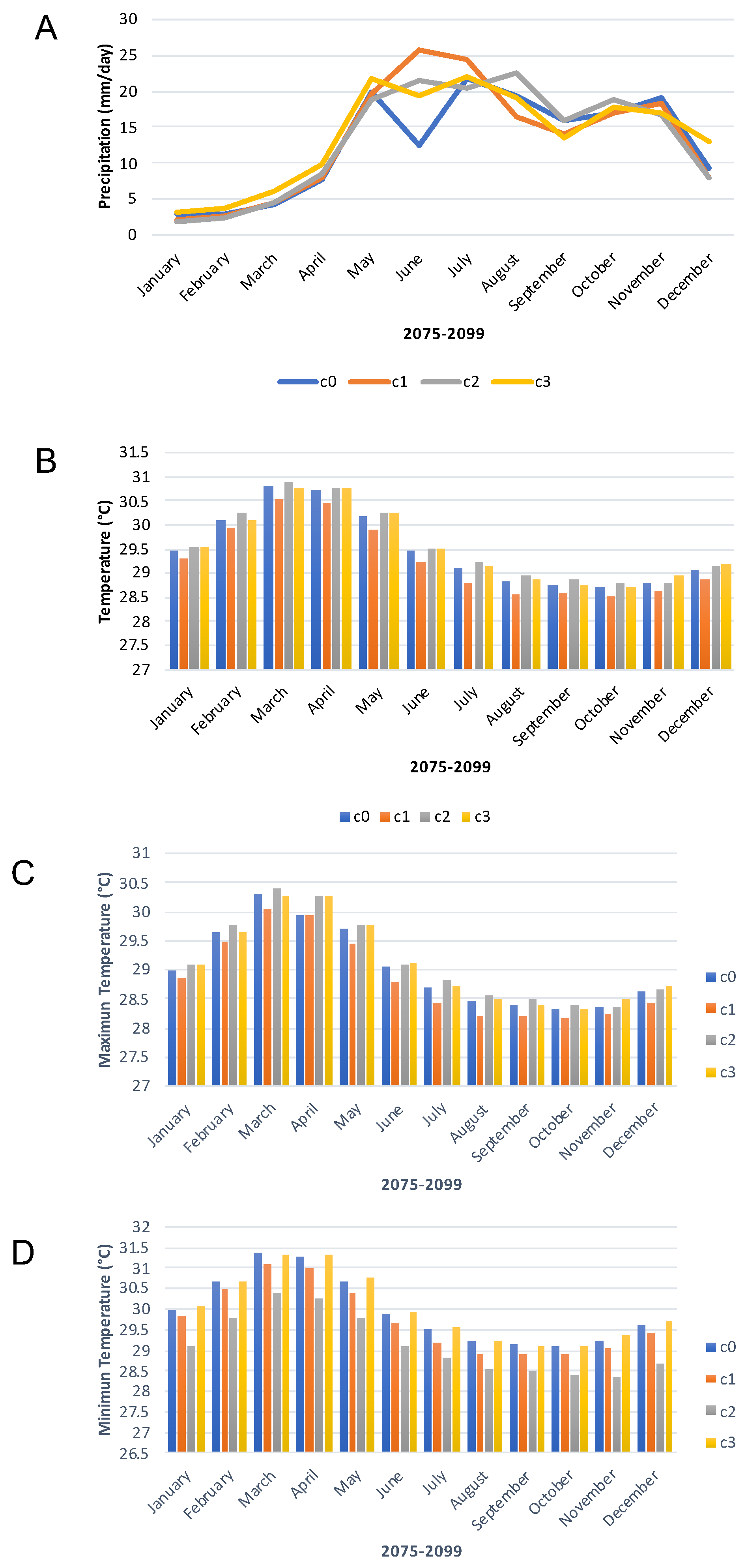
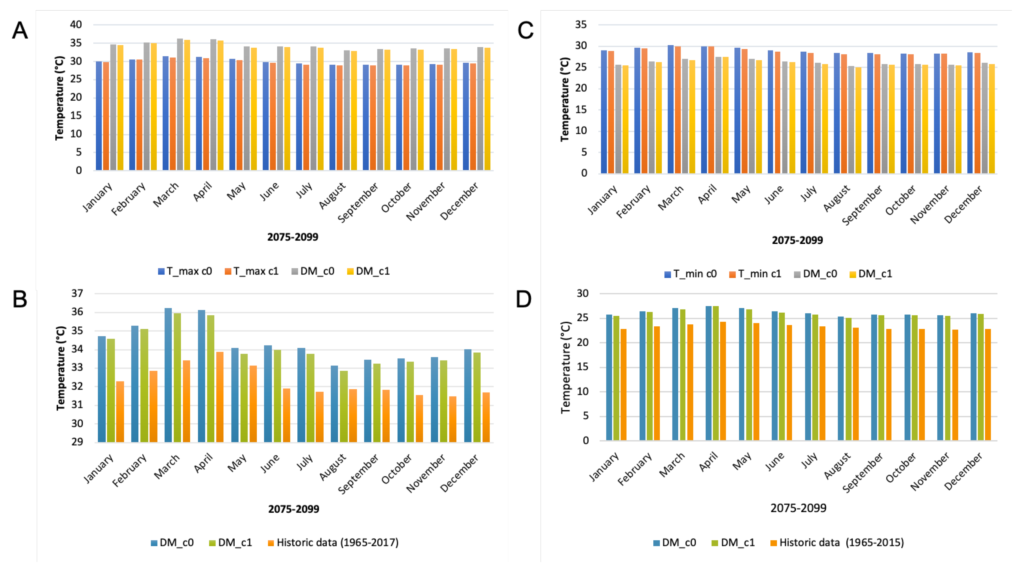
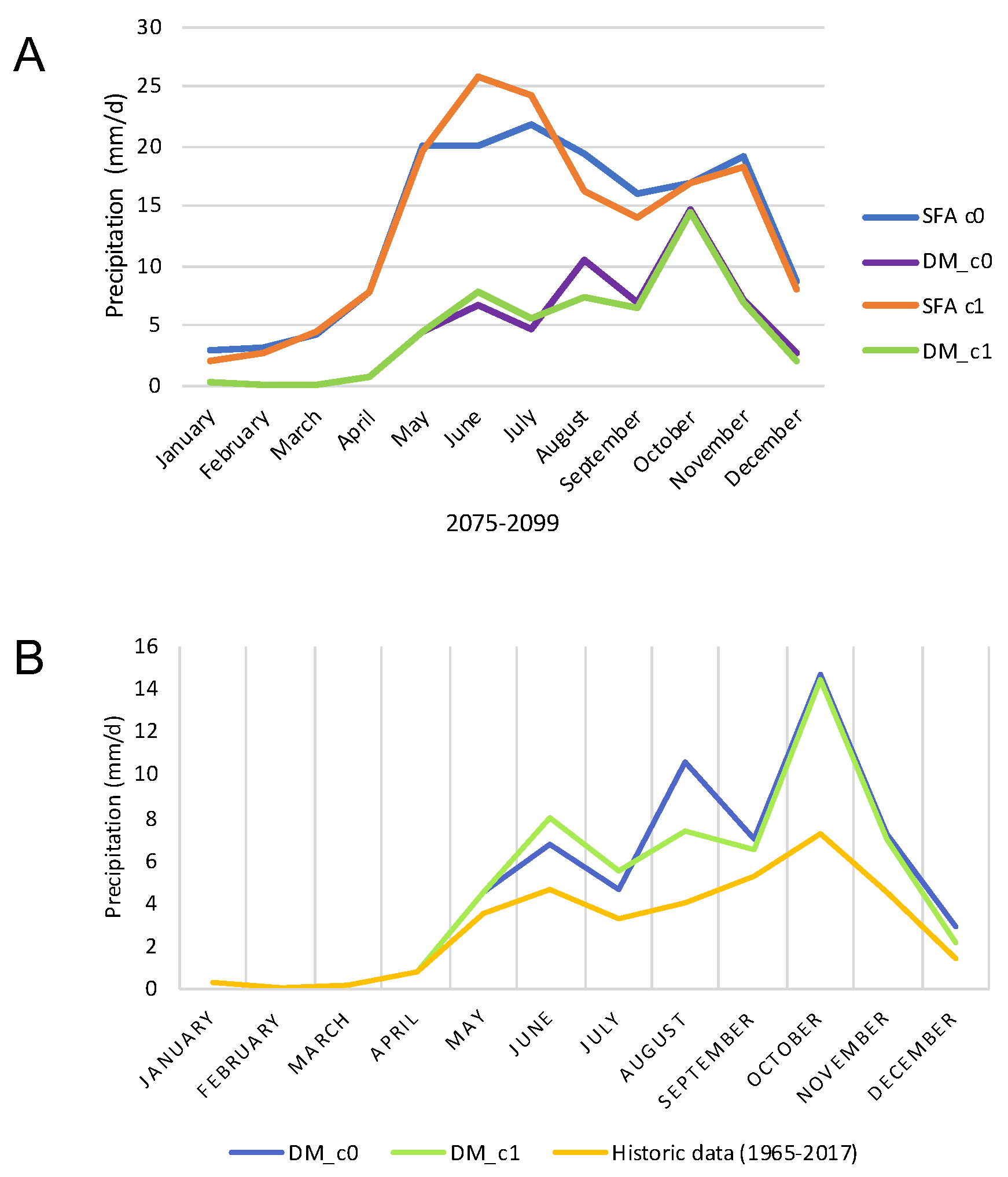
In this work, projected variables precipitation and temperature, from the MRI-AGCM 3.2 model, were studied in the Azuero region. Results confirmed that an increase in precipitation will be appreciated in the region at the end of the century [50]. More specifically, daily precipitation is projected to go up on average >15mm and temperatures will rise above 26 C and up to 36 C. Regarding localities, future precipitation projections are adjusted for localities north of Azuero region with respect to the C0 SST-ensemble. Future precipitation projections are adjusted for the localities south of Azuero with respect to SST-ensembles C1, C2, and C3.
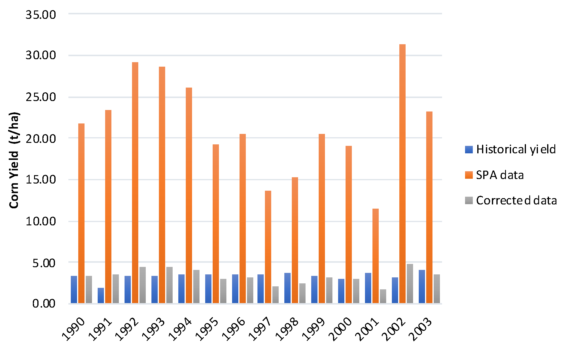
Simple correction was used to reduce the yield on the present time projections (SPA). The Delta Method was used to reduce the biases of the future climate estimates (SFA), for both variables precipitation and temperature. In the case of the maximum temperature, the values increase with respect to the corrected ones. The regression model tends to underestimate the maximum projected temperature and overestimate the minimum projected temperature. Not surprisingly, the lowest yields are found for all SST-ensemble for the later planting date. More interestingly, the yield model showed that for the C0, C2, and C3 SST-ensembles, the yield will double, while for the C1 SST-ensemble predicts, an average of 5% decrease for the period. This suggests that while the yield model shows that the production will be doubled, this change is sensitive to the future sea surface temperature distribution.
As future work, in terms of the agronomic model, a longer time series could be used to calculate maize yield. In this new model, it would be sensible to include the number of plants that exist at harvest time, to adjust the expected yield to the number of maize plants per hectare. This number now amounts to 65,000 per hectare and is a crucial factor to determine the yield.
Another important point would be to have data on irrigated maize, to be able to have a model that predicts the yield without water deficiencies. This will help to further separate the effect of rainfall and temperature, since for the regression model for the Azuero Region, rainfall captures more the variability of the response of the grain yield than temperature. This is in part due to its greater variation. In that same vein a model can incorporate a different treatment of variables, for instance de-trending of dependent and independent variables, log-transformation of the yield variable), to provide additional information about on how to determine the independent effect of temperature and precipitation on the crop yield, on present and future time.
Precipitation is well studied phenomenon in Panama, mostly for ensuring its availability for the functioning of the Panama Canal and the water cycle on the Canal watershed. However, other variables that are important for crop growth, for instance, VPD, solar radiation, and UV rays, which are important for maize, have not been projected in the end-of-century period. These variables should be incorporated into newer models as they become available to the research community.
Moreover, it is known that the CO 2 fertilization effect [51] is not well managed in statistical crop models [14]. Subsequent models need to include this component either by making an ensemble of both process-based and statistical crop models as suggested by Roberts et al. [13] and Lobell et al. [11], subtracting the effect of CO 2 from having yields under different RCPs [10], calculating it from a multi model comparison [5], or estimating it on-site as are done with the rain-forest in Barro Colorado Island in Panama [52].
Finally, it is important to state that this study and similar studies are of great relevance; The Azuero Region alone is responsible for over 95% of the maize grown in the country, with 18,000 hectares produced annually and a total production of 45,000 tons of grains per year [49]. Therefore, all mitigation efforts and efforts to understand future climates and their implications are very for the sovereignty and food security of Panama.

Author Contributions

Conceptualization, M.M.M., R.P., T.N., S.K., R.G., and J.E.S.-G.; methodology, M.M.M., T.N., S.K., R.G., and J.E.S.-G.; software, M.M.M., R.P., T.N., S.K., R.G., and J.E.S.-G.; validation, M.M.M., R.P., T.N., S.K., R.G., and J.E.S.-G.; resources, R.P., T.N., S.K., R.G., and J.E.S.-G.; writing–original draft preparation, M.M.M. and J.E.S.-G.; writing–review and editing, M.M.M., R.P., T.N., S.K., R.G., and J.E.S.-G.; visualization, M.M. and J.E.S.-G.; supervision of students, J.E.S.-G. All authors have read and agreed to the published version of the manuscript.

Funding

M.M.M. was supported by a scholarship of the Programa de Fortalecimiento de los Postgrados Nacionales from the National Secretariat for Science, Technology and Innovation (SENACYT). T.N. had funds and support from the JSPS KAKENHI Grant Numbers-in-Aid for Specially Promoted Research (grant number, 16H06291 and 20K12154), and support from Theme C of the TOUGOU program (JPMXD0717935498) funded by the Japanese Ministry of Education, Culture, Sports, Science and Technology. R.P. and J.E.S.-G. had the scientific support from SENACYT through projects: APY-GC-2016-18, FID-2016-275 and EIE-2018-16; and throught the Sistema Nacional de Investigación (SNI) of SENACYT. The APC was covered by J.E.S.-G. SNI funds (Contract No. 129-2018).

Acknowledgments

The authors acknowledge administrative support provided by the Universidad Tecnológica de Panamá.

Conflicts of Interest

The authors declare no conflict of interest.

Appendix A. Regression Model Validation

As introduced in Section 2.4.1, the model corresponds to multiple regression using material Pioneer 30F-35 yield of the plots in dry land for the 2015–2017 period. The regression model takes into account the precipitation and average temperature in the third and fourth stages, with all variables being significant at p < 0.10, and with precipitation having a greater influence in the yields, as shown in Table A1.
Table A1. Regression Model taken into account observations from 2015 to 2017 (3 years).
VariableDFParameter EstimateStandard Errort-Valuep >|t|
PRE310.02820.012.90.03
PRE410.04460.013.080.03
TEMP31−2.07860.96−2.160.08
TEMP412.10930.952.210.08
As for model validation (or out-of-sample validation) of the regression model, the yield of 2018 and 2019 was used in three different planting dates, results shown in Table A2.
Validation results with the regression model show that on average the residual value amounted to 1.47 t ha 1 . More importantly, the predicted yields were comparable, with the observed yields, and even more interesting and effect of planting date, that is difference between planting on an earlier date and later date is distinguishable, and the yield is reduced.
Table A2. Residual Analysis of Yield for 2018 and 2019 for the model.
YearPlanting DateObserved YieldPredicted YieldResidual
21 August9.426.692.73
23 September6.693.263.42
201810 October1.310.930.38
21 August7.955.202.75
23 September6.153.672.48
201910 October1.494.39−2.90
Average1.47

References

  1. Adams, R.M.; Hurd, B.H.; Lenhart, S.; Leary, N. Effects of global climate change on agriculture: An interpretative review. Clim. Res. 1998, 11, 19–30. [Google Scholar] [CrossRef] [Green Version]
  2. Nelson, G.C.; Valin, H.; Sands, R.D.; Havlík, P.; Ahammad, H.; Deryng, D.; Elliott, J.; Fujimori, S.; Hasegawa, T.; Heyhoe, E.; et al. Climate change effects on agriculture: Economic responses to biophysical shocks. Proc. Natl. Acad. Sci. USA 2014, 111, 3274–3279. [Google Scholar] [CrossRef] [PubMed] [Green Version]
  3. Morton, J.F. The impact of climate change on smallholder and subsistence agriculture. Proc. Natl. Acad. Sci. USA 2007, 104, 19680–19685. [Google Scholar] [CrossRef] [PubMed] [Green Version]
  4. Lobell, D.B.; Field, C.B. Global scale climate–crop yield relationships and the impacts of recent warming. Environ. Res. Lett. 2007, 2, 014002. [Google Scholar] [CrossRef]
  5. Rosenzweig, C.; Elliott, J.; Deryng, D.; Ruane, A.C.; Müller, C.; Arneth, A.; Boote, K.J.; Folberth, C.; Glotter, M.; Khabarov, N.; et al. Assessing agricultural risks of climate change in the 21st century in a global gridded crop model intercomparison. Proc. Natl. Acad. Sci. USA 2014, 111, 3268–3273. [Google Scholar] [CrossRef] [Green Version]
  6. Gregory, P.J.; Ingram, J.S.; Brklacich, M. Climate change and food security. Philos. Trans. R. Soc. B Biol. Sci. 2005, 360, 2139–2148. [Google Scholar] [CrossRef]
  7. Pipitpukdee, S.; Attavanich, W.; Bejranonda, S. Climate Change Impacts on Sugarcane Production in Thailand. Atmosphere 2020, 11, 408. [Google Scholar] [CrossRef] [Green Version]
  8. Mall, R.; Gupta, A.; Sonkar, G. Effect of climate change on agricultural crops. In Current Developments in Biotechnology and Bioengineering; Elsevier: Amsterdam, The Netherlands, 2017; pp. 23–46. [Google Scholar]
  9. Jones, P.G.; Thornton, P.K. The potential impacts of climate change on maize production in Africa and Latin America in 2055. Glob. Environ. Chang. 2003, 13, 51–59. [Google Scholar] [CrossRef]
  10. Ruane, A.C.; Cecil, L.D.; Horton, R.M.; Gordón, R.; McCollum, R.; Brown, D.; Killough, B.; Goldberg, R.; Greeley, A.P.; Rosenzweig, C. Climate change impact uncertainties for maize in Panama: Farm information, climate projections, and yield sensitivities. Agric. For. Meteorol. 2013, 170, 132–145. [Google Scholar] [CrossRef]
  11. Lobell, D.B.; Asseng, S. Comparing estimates of climate change impacts from process-based and statistical crop models. Environ. Res. Lett. 2017, 12, 015001. [Google Scholar] [CrossRef]
  12. Lobell, D.B.; Burke, M.B. On the use of statistical models to predict crop yield responses to climate change. Agric. For. Meteorol. 2010, 150, 1443–1452. [Google Scholar] [CrossRef]
  13. Roberts, M.J.; Braun, N.O.; Sinclair, T.R.; Lobell, D.B.; Schlenker, W. Comparing and combining process-based crop models and statistical models with some implications for climate change. Environ. Res. Lett. 2017, 12, 095010. [Google Scholar] [CrossRef]
  14. Kogo, B.K.; Kumar, L.; Koech, R.; Langat, P. Modelling Impacts of Climate Change on Maize (Zea mays L.) Growth and Productivity: A Review of Models, Outputs and Limitations. J. Geosci. Environ. Prot. 2019, 7, 76. [Google Scholar]
  15. Holzkämper, A.; Calanca, P.; Fuhrer, J. Statistical crop models: Predicting the effects of temperature and precipitation changes. Clim. Res. 2012, 51, 11–21. [Google Scholar] [CrossRef] [Green Version]
  16. Holzkämper, A.; Calanca, P.; Honti, M.; Fuhrer, J. Projecting climate change impacts on grain maize based on three different crop model approaches. Agric. For. Meteorol. 2015, 214, 219–230. [Google Scholar] [CrossRef]
  17. Auffhammer, M.; Schlenker, W. Empirical studies on agricultural impacts and adaptation. Energy Econ. 2014, 46, 555–561. [Google Scholar] [CrossRef] [Green Version]
  18. Nakayama, K.; Beitia, C.; Vallester, E.; Pinzon, R.; Fábrega, J.; Nakaegawa, T.; Maruya, Y.; Espinosa, J.; Olmedo, B.; Kato, J. Increase in simple precipitation intensity index in Panama. J. Jpn. Soc. Civ. Eng. Ser. B1 (Hydraulic Eng.) 2012, 68, I_163–I_168. [Google Scholar] [CrossRef] [Green Version]
  19. Beitia, C. Aplicación del Modelo del Clima Global MRI-AGCM en la Proyección de Precipitación en la República de Panamá. Bachelor’s Thesis, Faculty of Civil Engineering, Universidad Tecnologica Panamá, Panama City, Panama, 2012. [Google Scholar]
  20. Fábrega, J.; Nakaegawa, T.; Pinzón, R.; Nakayama, K.; Arakawa, O. Hydroclimate projections for Panama in the late 21st Century. Hydrol. Res. Lett. 2013, 7, 23–29. [Google Scholar]
  21. Kusunoki, S.; Nakaegawa, T.; Pinzón, R.; Sanchez-Galan, J.E.; Fábrega, J.R. Future precipitation changes over Panama projected with the atmospheric global model MRI-AGCM3. 2. Clim. Dyn. 2019, 53, 5019–5034. [Google Scholar] [CrossRef]
  22. Espinosa, D.; Mendez, A.; Madrid, I.; Rivera, R. Assessment of climate change impacts on the water resources of Panama: The case of the La Villa, Chiriqui and Chagres River Basins. Clim. Res. 1997, 9, 131–137. [Google Scholar] [CrossRef]
  23. Hobeika, M.; Wagner, A.C. The Impacts of Climate Change on Agriculture in Tierras Altas, Panama and Recommendations for Adaptation: Perspectives of Local Farmers; Panama Field Study Semester; McGill University: Montreal, QC, Canada, April 2018. [Google Scholar]
  24. García, K.; Del Castillo, L.; Saavedra, C. Analysis of climate anomalies for La Villa river basin, Panama, based on RCP scenarios. I+ D Tecnológico 2020, 16, 84–90. [Google Scholar]
  25. Gordón, R. Los Granos Básicos y la Variabilidad Climática en Azuero: Caso Maíz; Primer Congreso Científico Universidad de Panamá, Centro Regional Universitario de Los Santos: Las Tablas, Panama, 2014. [Google Scholar] [CrossRef]
  26. Empresa de Transmision Electrica S.A., (ETESA). Datos Climaticos Historicos. 2019. Available online: http://www.hidromet.com.pa/clima_historicos.php (accessed on 2 February 2019).
  27. Gordón-Mendoza, R. Variabilidad Climática y su Efecto en la Producción del Maíz; Instituto de Investigación Agropecuaria de Panamá: Calle Carlos Lara, Panama, 2020; 48p. [Google Scholar]
  28. Mizuta, R.; Yoshimura, H.; Murakami, H.; Matsueda, M.; Endo, H.; Ose, T.; Kamiguchi, K.; Hosaka, M.; Sugi, M.; Yukimoto, S.; et al. Climate simulations using MRI-AGCM3. 2 with 20-km grid. J. Meteorol. Soc. Japan. Ser. II 2012, 90, 233–258. [Google Scholar] [CrossRef] [Green Version]
  29. Mizuta, R.; Oouchi, K.; Yoshimura, H.; Noda, A.; Katayama, K.; Yukimoto, S.; Hosaka, M.; Kusunoki, S.; Kawai, H.; Nakagawa, M. 20-km-mesh global climate simulations using JMA-GSM model—Mean climate states. J. Meteorol. Soc. Japan. Ser. II 2006, 84, 165–185. [Google Scholar] [CrossRef] [Green Version]
  30. Kitoh, A.; Kusunoki, S.; Nakaegawa, T. Climate change projections over South America in the late 21st century with the 20 and 60 km mesh Meteorological Research Institute atmospheric general circulation model (MRI-AGCM). J. Geophys. Res. Atmos. 2011, 116, 21. [Google Scholar] [CrossRef]
  31. Nakaegawa, T.; Kitoh, A.; Kusunoki, S.; Murakami, H.; Arakawa, O. Hydroclimate change over Central America and the Caribbean in a global warming climate projected with 20-km and 60-km mesh MRI atmospheric general circulation models. Pap. Meteorol. Geophys 2014, 65, 15. [Google Scholar] [CrossRef] [Green Version]
  32. Change, I.C. Synthesis Report. Contribution of working groups I. II III Fifth Assess. Rep. Intergov. Panel Clim. Chang. 2014, 151. [Google Scholar]
  33. Murakami, H.; Mizuta, R.; Shindo, E. Future changes in tropical cyclone activity projected by multi-physics and multi-SST ensemble experiments using the 60-km-mesh MRI-AGCM. Clim. Dyn. 2012, 39, 2569–2584. [Google Scholar] [CrossRef] [Green Version]
  34. Murakami, H.; Sugi, M.; Kitoh, A. Future changes in tropical cyclone activity in the North Indian Ocean projected by high-resolution MRI-AGCMs. Clim. Dyn. 2013, 40, 1949–1968. [Google Scholar] [CrossRef] [Green Version]
  35. Ministerio de Desarrollo Agropecuario. Cierre Agrícola 2018–2019. 2020. Available online: https://www.mida.gob.pa/upload/documentos/cierre___2018-2019_ok.pdf (accessed on 15 August 2020).
  36. Ministerio de Desarrollo Agropecuario. Serie Histórica de los Rubros Agrícolas 1992–2019. 2019. Available online: https://www.mida.gob.pa/direcciones/direcciones_nacionales/direcci-n-de-agricultura/serie-hist-rica-de-los-rubros-agr-colas-1992-2019.html (accessed on 3 February 2019).
  37. Sáez-Cigarruista, A.E.; Gordón-Mendoza, R.; Núñez-Cano, J.I.; Jaén-Villarreal, J.E.; Franco-Barrera, J.E.; Ramos-Manzané, F.; Ávila-Guevara, A. Coeficientes genéticos de dos cultivares de maíz, Azuero-Panamá. Cienc. Agropecu. 2018, 29, 80–99. [Google Scholar]
  38. Denmead, O.; Shaw, R.H. The Effects of Soil Moisture Stress at Different Stages of Growth on the Development and Yield of Corn 1. Agron. J. 1960, 52, 272–274. [Google Scholar] [CrossRef]
  39. McWilliams, D.A.; Berglund, D.R.; Endres, G. Corn growth and management quick guide. In North Dakota Cooperative Extension Service; North Dakota State University: Fargo, ND, USA, 1999; pp. 1–8. [Google Scholar]
  40. Sah, R.; Chakraborty, M.; Prasad, K.; Pandit, M.; Tudu, V.; Chakravarty, M.; Narayan, S.; Rana, M.; Moharana, D. Impact of water deficit stress in maize: Phenology and yield components. Sci. Rep. 2020, 10, 2944. [Google Scholar] [CrossRef] [PubMed]
  41. Kranz, W.L.; Irmak, S.; Van Donk, S.J.; Yonts, C.D.; Martin, D.L. Irrigation management for corn. Neb Guid. Univ. Nebraska Linc. 2008, 10, 1–8. [Google Scholar]
  42. Araya, A.; Kisekka, I.; Lin, X.; Prasad, P.V.; Gowda, P.; Rice, C.; Andales, A. Evaluating the impact of future climate change on irrigated maize production in Kansas. Clim. Risk Manag. 2017, 17, 139–154. [Google Scholar] [CrossRef]
  43. Wang, L.; Chen, W. Equiratio cumulative distribution function matching as an improvement to the equidistant approach in bias correction of precipitation. Atmos. Sci. Lett. 2014, 15, 1–6. [Google Scholar] [CrossRef]
  44. Piani, C.; Weedon, G.; Best, M.; Gomes, S.; Viterbo, P.; Hagemann, S.; Haerter, J. Statistical bias correction of global simulated daily precipitation and temperature for the application of hydrological models. J. Hydrol. 2010, 395, 199–215. [Google Scholar] [CrossRef]
  45. Piani, C.; Haerter, J.; Coppola, E. Statistical bias correction for daily precipitation in regional climate models over Europe. Theor. Appl. Climatol. 2010, 99, 187–192. [Google Scholar] [CrossRef] [Green Version]
  46. Madrigal, J.; Flores Fernandez, G.; Solera, A.; Abreu, J. Corrección del sesgo en los estadísticos de las series de precipitación de cambio climático, en la cuenca del río Angulo. In Proceedings of the 5th Young Water Professionals Conference, Morelia, Mexico, 5–7 July 2017. [Google Scholar]
  47. Cannon, A.J.; Sobie, S.R.; Murdock, T.Q. Bias correction of GCM precipitation by quantile mapping: How well do methods preserve changes in quantiles and extremes? J. Clim. 2015, 28, 6938–6959. [Google Scholar] [CrossRef]
  48. Hidalgo, H.; Alfaro, E.; Quesada-Montano, B. Observed (1970–1999) climate variability in Central America using a high-resolution meteorological dataset with implication to climate change studies. Clim. Chang. 2017, 141, 13–28. [Google Scholar] [CrossRef] [Green Version]
  49. Gordón Mendoza, R.; Franco Barrera, J.E.; Camargo Buitrago, I. Impacto de la tecnología generada en el cultivo de maíz para la Región de Azuero. Cienc. Agropecu. 2016, 24, 1–18. [Google Scholar]
  50. Nakaegawa, T.; Arakawa, O.; Kamiguchi, K. Investigation of climatological onset and withdrawal of the rainy season in Panama based on a daily gridded precipitation dataset with a high horizontal resolution. J. Clim. 2015, 28, 2745–2763. [Google Scholar] [CrossRef]
  51. Dhakhwa, G.B.; Campbell, C.L.; LeDuc, S.; Cooter, E. Maize growth: Assessing the effects of global warming and CO2 fertilization with crop models. Agric. For. Meteorol. 1997, 87, 253–272. [Google Scholar] [CrossRef]
  52. Sugasti, L.; Pinzón, R. First Approach of Abiotic Drivers of Soil CO2 Efflux in Barro Colorado Island, Panama. Air Soil Water Res. 2020, 13, 1178622120960096. [Google Scholar] [CrossRef]
Publisher’s Note: MDPI stays neutral with regard to jurisdictional claims in published maps and institutional affiliations.
Figure 1. Location of the Azuero Region of Panama. Source: The authors.
Atmosphere 11 01097 g001
Figure 2. Maize Yield for the Azuero region (1990–2017). Source: MIDA [36].
Atmosphere 11 01097 g002
Figure 3. Comparison of monthly averages in the 2075–2099 period under different SST schemes (C0 and C1) and the RCP8.5 trajectory. Precipitation month by month (A), Average Temperature month by month (B), and Minimum and Maximum Temperature for C0 and C1 SST Schemes (C,D).
Atmosphere 11 01097 g003
Figure 4. Historical, Projected Present time data, and Corrected Present time maize yield in the 1990–2003 period.
Atmosphere 11 01097 g004
Figure 5. Comparison of the monthly temperature for projected estimates under the C0 and C1 SST-ensembles and their respective corrected counterparts: Monthly maximum temperatures (A), Monthly minimum temperatures (C). Comparison of the corrected temperature to the historical meteorological data: maximum temperatures (B), minimum temperatures (D).
Atmosphere 11 01097 g005
Figure 6. Comparison of monthly averages of daily precipitation for data projected by the model (RCP8.5 trajectory and C0 and C1 SST schemes) and the respective data corrected using Delta Method (A). Comparison of the corrected precipitation values with the historical averages (B).
Atmosphere 11 01097 g006
Table 1. Future time yields in tha 1 for C0 and C1 SST-ensemble and for early, mid, and late planting dates.
C0C1
Year21 August23 September10 October21 August23 September10 October
207536.318.013.418.113.513.4
207640.411.016.728.116.212.9
207729.530.814.422.519.810.0
20787.67.62.53.74.33.7
207916.350.224.822.930.314.1
208036.432.110.720.032.923.6
208128.624.96.811.917.015.5
208229.143.911.115.417.65.5
208337.256.416.826.328.513.9
208429.327.117.324.119.111.8
208533.939.017.922.820.95.4
208623.638.119.522.621.910.9
208728.124.310.311.514.59.9
208850.730.612.920.816.77.5
208937.362.813.516.828.95.8
209036.330.14.812.518.27.7
209163.260.934.848.535.920.4
209224.322.615.520.018.010.6
209315.212.24.25.26.74.2
209432.445.719.224.227.921.1
209540.122.220.934.922.114.6
209649.628.318.729.116.19.7
209738.022.616.931.925.714.2
209820.024.85.66.212.88.6
209924.263.616.624.3
Average32.333.214.620.720.411.4
Table 2. Future time yields in tha 1 for C2 and C3 SST-ensemble and for early, mid, and late planting dates.
C2C3
Year21 August23 September10 October21 August23 September10 October
207527.310.77.623.729.924.2
207634.619.211.834.618.97.3
207727.315.910.211.514.213.4
20786.13.13.08.86.34.5
207931.031.718.630.731.223.8
208032.117.211.124.112.112.9
208133.117.516.648.218.05.4
208221.65.53.731.826.620.5
208334.130.825.233.960.048.3
208435.434.824.230.820.615.8
208535.642.128.135.725.420.0
208622.216.815.434.713.711.0
208719.45.44.118.412.29.5
208849.421.28.853.227.516.3
208930.225.911.220.824.117.4
209016.96.85.334.222.213.4
209155.634.925.624.928.221.2
209231.128.223.844.346.131.1
209318.22.92.120.011.18.7
209438.715.013.234.155.136.6
209531.520.218.930.322.820.4
209630.813.310.150.738.425.7
209731.721.211.734.222.615.6
209841.213.85.314.77.56.3
209936.825.354.934.1
Average30.919.213.131.325.217.9
Table 3. Average change in percentage from simulated baseline for 5-year period at the End-of-Century for C0 and C1 SST-Ensembles.
C0C1
Period21 August23 September10 October21 August23 September10 October
2075–207920%8%−34%−12%−23%−50%
2080–208448%70%−42%−10%6%−35%
2085–208960%79%−32%−13%−5%−64 %
2090–209458%58%−28%2%−2%−41%
2095–209958%49%−29%9%−7%−46%
2075–209949%53%-33%−5%−6%−47%
Table 4. Average change in percentage from simulated baseline for 5-year period at the End-of-Century for C2 and C3 SST-Ensembles.
C2C3
Period21 August 23 September10 October21 August23 September10 October
2075–207916%−26%−53%1%−7%−33%
2080–208444%−2%−25%56%27%−5%
2085–208945%3%−38%50%−5%−32%
2090–209448%−19%−36%45%50%2%
2095–209958%−13%−47%70%16−22%
2075–209942%−12%−39%44%16%−18%

