


INTRODUCTION
For meaningful interpretation of the recorded signals in ice cores from glacier archives, accurate dating is essential. Radiocarbon (14C) is a powerful tool for dating and is widely applied in different fields (Libby Reference Libby1954; Stuiver and Suess Reference Stuiver and Suess1966; Reimer et al. Reference Reimer, Bard and Bayliss2013). For ice cores from high-alpine glaciers 14C-dating is particularly valuable for the ice in the bottom part, where strong thinning of annual layers prevents the use of annual layer counting or the assignment of reference horizons for dating (Thompson et al. Reference Thompson, Davis and Mosley-Thompson1998; Schwikowski et al. Reference Schwikowski, Brütsch and Gäggeler1999a). The 14C half-life of 5730 yr allows covering the typical age range of alpine ice cores. 14C dating of water insoluble organic carbon (WIOC) from glacier ice has been well established. Samples of 10 μg WIOC can now be dated with reasonable uncertainty, requiring less than 1 kg of ice from typical mid-latitude and low-latitude glaciers (Jenk et al. Reference Jenk, Szidat and Schwikowski2007, Reference Jenk, Szidat and Bolius2009; Sigl et al. Reference Sigl, Jenk and Kellerhals2009; Uglietti et al. Reference Uglietti, Zapf and Jenk2016). However, the low WIOC concentration in glaciers remote from sources, e.g. glaciers in the polar regions, puts a limit to this application. Because the concentrations of dissolved organic carbon (DOC) are around a factor 5 higher (10–100 ppbC, Legrand et al. Reference Legrand, Preunkert and Jourdain2013a, Reference Legrand, Preunkert and May2013b), using this fraction promises to allow an extension of this approach to new sites and generally reducing the achievable analytical (dating) uncertainty.
In addition to dating, 14C has proved to be a powerful tool for source apportionment studies, i.e. to distinguish biogenic and fossil source contributions (Szidat et al. Reference Szidat, Jenk and Synal2006; Zhang et al. Reference Zhang, Perron and Ciobanu2012). Alpine ice cores allow access to continuous records of atmospheric pollution back to the preindustrial era in the regions where the majority of humans live (Schwikowski et al. Reference Schwikowski, Döscher and Gäggeler1999b; Eichler et al. Reference Eichler, Tobler and Eyrikh2012, Reference Eichler, Gramlich and Kellerhals2015). A first long-term trend in concentrations separated into the contribution from fossil fuel and biogenic sources of atmospheric organic carbonaceous particles was reconstructed from an ice core at the Fiescherhorn glacier (Swiss Alps; Jenk et al. Reference Jenk, Szidat and Schwikowski2006). In contrast to WIOC, which mainly consists of primary organic aerosol from direct emissions, water soluble organic carbon (WSOC) originates in large part from secondary organic aerosols (SOAs) formed in the atmosphere from volatile organic precursor compounds (Gelencsér et al. Reference Gelencsér, May and Simpson2007). WSOC is a major fraction of organic aerosols in the atmosphere; however, its sources are not well constrained (Pio et al. Reference Pio, Legrand and Oliveira2007). WSOC in snow and ice is only one part of the DOC which is analyzed and additionally contains gaseous organics taken up during snowfall (Legrand et al. Reference Legrand, Preunkert and May2013b). Studying DOC along with its 14C content in samples from ice cores will allow additional insight into historical natural and anthropogenic contributions to the organic carbon content of atmospheric aerosols.
Only very few long-term records of DOC concentrations, and even fewer in combination with the 14C content, exist to date. To our knowledge all of these records were derived from ice cores (Preunkert et al. Reference Preunkert, Legrand and Stricker2010; Legrand et al. Reference Legrand, Preunkert and May2013b; May et al. Reference May, Wagenbach and Hoffmann2013). For studies of DOC in ice cores, one of the major limitations is the rather large demand of sample amount along with relatively low extraction efficiency and the threat of sample contamination (Preunkert et al. Reference Preunkert, Legrand and Stricker2010; Legrand et al. Reference Legrand, Preunkert and May2013b; May et al. Reference May, Wagenbach and Hoffmann2013). With the current state of the art of 14C analysis with accelerator mass spectrometry (AMS) that allows the direct measurement of gaseous CO2 samples, carbon sample masses of as low as 3 μg are sufficient (Ruff et al. Reference Ruff, Wacker and Gäggeler2007). Still, this translates to typical ice sample masses of several hundred grams for DO14C analyses. However, preceding AMS analysis, DOC has to be oxidized to CO2. In contrast to high-temperature combustion or wet-chemical oxidation techniques, the use of ultraviolet (UV) photochemical oxidation has the advantage of being suitable for large volumes of sample with low carbon content (Beaupré et al. Reference Beaupré, Druffel and Griffin2007). It was applied by Singer et al. (Reference Singer, Fasching and Wilhelm2012) to determine the DO14C content of ice samples from different glaciers in the European Alps. However, their method has a limited carbon yield of 50% (Steier et al. Reference Steier, Fasching and Mair2013). May (Reference May2009) and May et al. (Reference May, Wagenbach and Hoffmann2013) developed a setup for 14C microanalysis of glacier ice and applied it to several ice core samples, but unexpected super-modern 14C values led to inconclusive results. It should be noted that a straightforward analysis of DOC is challenging due to its vulnerability to contamination (Legrand et al. Reference Legrand, Preunkert and Jourdain2013a). Ice cores can potentially be contaminated during drilling, storage, and sample processing. Besides, DOC consists of a large part of mono- and di-carboxylic acids that are ubiquitous in ambient and laboratory air (Legrand et al. Reference Legrand, Preunkert and May2013b). Therefore, it is vital to ensure ultra-clean sample preparation and extraction with a low and stable process blank for reliable 14C analysis of DOC. Here, we present such an approach with a new extraction setup for DOC concentration and 14C analysis in low-concentration ice core samples. Our extraction system is designed for samples with volumes of up to ~350 mL and concentrations as little as 25 ppbC DOC (equals to 25 μg C kg–1 ice).
EXPERIMENTAL
Extraction Setup
Figure 1 shows an overview scheme of the complete DOC extraction setup (Schindler Reference Schindler2017). This setup allows handling of the entire sample treatment under inert gas conditions (≥99.999% helium gas, further purified by a homemade getter oven) in order to extract carbon masses of as little as a few micrograms, while aiming to avoid potential contamination during analysis. The getter oven consists of an insulated, resistively heated Inconel (a high temperature resistant nickel-chromium-based super-alloy) tube filled with 15 g tantalum wire. Helium is used as carrier gas in the entire setup. Furthermore, all parts in contact with the sample when in its liquid form were fabricated modularly from either glass or quartz glass to allow thorough cleaning and reduction of memory effects compared to stainless steel. To minimize outgassing or out-washing of organic carbon into the sample, no lubricants are used. The major system components, highlighted in green text in Figure 1, are described in detail in the following:
The glass melting vessel (custom made by GlasKeller AG, Switzerland) with an inner diameter with an inner diameter of 100 mm has a volume of around 1.3 L (Figure 2a). A support holds the vessel and fixes the stainless steel cover plate to the vessel by spring tension. The flange connection is sealed by a PFA coated O-ring. As illustrated in the sketch, the cover plate gives access to four thread connectors (¼ inch): (1) the helium supply, (2) a metering valve (SS-BNTS6MM, Swagelok, USA) with a bubble counter (GlasKeller AG, Switzerland) that acts as a vent with water ballast (vent 1), (3) a manometer for pressure monitoring (PBMN-25B11AA14402201000, Baumer Electric AG, Switzerland), and (4) the ultra-pure water (UPW) supply. The UPW dispenser system consists of a glass bottle filled with UPW (Sartorius, 18.2 MΩ×cm) and connected by PFA tubes to both the helium supply and the cover plate. Applying pressure via the helium supply allows pushing the desired amount of UPW to the melting vessel.
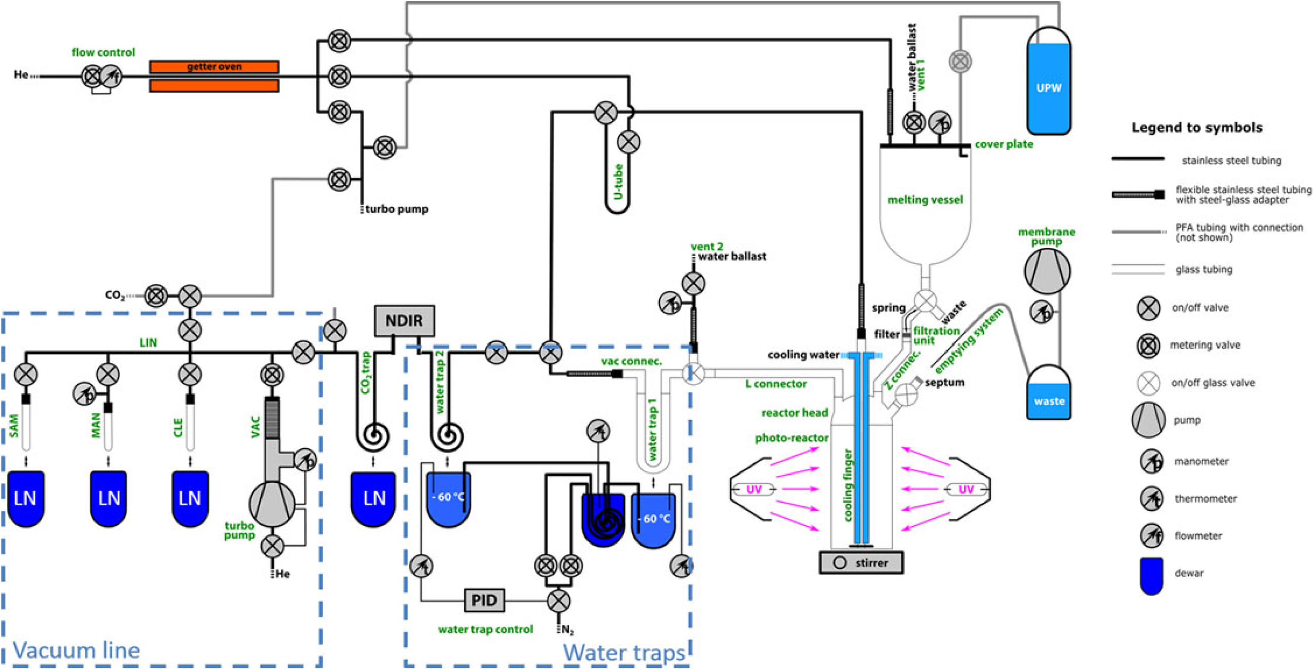
Figure 1 Schematic of the complete DOC extraction setup. Green text labels individual components. UPW (ultra-pure water), LN (liquid nitrogen), NDIR (CO2 detector), LIN (vacuum manifold), VAC (pump manifold), CLE (cleaning tube), MAN (manometry cell), SAM (sampling tube).
The filtration unit is shaped as an adapter piece from glass spherical joint (SJ) 41/25 to SJ 19/7 (Figure 2a). In the center, an 8-mm-diameter frit (160–250 μm) acts as support for a pre-cleaned quartz fiber filter that was baked at 800°C for 2 hr (20 mm diameter, PALLFLEX Tissuquartz, 2500QAO-UP) and fixed onto the frit by a metal spring. The filter used for the separation of POC from the liquid sample is similar to the procedure for WIO14C analysis described in Jenk et al. (Reference Jenk, Szidat and Schwikowski2006). However, in contrast to the commonly used lab filtration unit described therein, this setup allows filtration under inert gas conditions, avoiding potential sample contamination from take-up and mixing of ambient air with the liquid sample during the filtration step.

Figure 2 View of (a) melting vessel, filtration valve and filtration unit, (b) the photo-reactor, reactor head and cooling finger. Italic text refers to the labeling introduced in Figure 1, bold text refers to connections or emphasizes special features.
The photo-reactor is a cylindrical quartz glass vessel (Qsil GmbH, Germany) (Figure 2b), and allows introduction of the filtered solution via a glass connector (Z connector). In the center of the reactor head, the cooling finger is inserted via a glass SJ 41/25 connection and reaches close to the base of the photo-reactor. The cooling finger has several functions and is constructed from three concentric glass tubes. The inner tube is connected to the helium supply. The outer two tubes serve for cooling water circulation in the cooling finger and in combination with external cooling of the photo-reactor by air ventilation is essential to control the sample temperature during photo-oxidation. For sample mixing, the promotion of homogeneous oxidation and efficient degassing, a magnetic stirrer is used. The magnetic stir bar is encapsulated in glass to avoid contamination (Beaupré et al. Reference Beaupré, Druffel and Griffin2007). Two UV lamps (MH-Module 250W Hg XL, Heraeus, Germany) are installed opposite of each other and enclose the reactor in a distance of 3 cm to the reactor walls. A box surrounds the UV lamps and reactor to prevent user-exposure to UV irradiation and ozone. This protection box further enhances the photon-yield because of its reflective aluminum construction. The emptying system consists of a long stainless steel needle, a glass bottle, and a membrane pump. For sample removal the stainless steel needle is introduced through a septum to the reactor and the sample is pumped out with a membrane pump.
Despite cooling with the cool finger, the liquid sample heats up to around 50°C during UV irradiation, resulting in an enhanced content of water vapor. For water removal, two cryogenic water traps are therefore added in front of the CO2 trap that is cooled with liquid nitrogen (LN). Water trap 1 (Figure 1) is a U-shaped glass tube (20 cm length, 10 mm inner diameter) filled with glass capillaries and water trap 2 is made from stainless steel tube bent to a coil (2 m length, ¼ inch outer diameter [OD], Swagelok). A PID temperature controller (Eurotherm Produkte AG, Switzerland) is used to stabilize both water traps at –60ºC by a controlled nitrogen gas transfer from a LN reservoir into the Dewar around the water traps, similar in principle to the system described in Jenk et al. (Reference Jenk, Rubino and Etheridge2016).
All components of the vacuum line (indicated as blue dashed box in Figure 1) are made from stainless steel tubes (¼ inch OD) and stainless steel fittings (Swagelok) allowing operation at high vacuum of about 10–7 mbar. A turbo-molecular pump (HiCube 80 Eco, Pfeiffer Vacuum AG, Germany) is connected to the vacuum line through a dosing valve (SS-6BMRG-MM-SC11, Swagelok). The vacuum line for CO2 sample purification and collection is similar to the one described in Szidat et al. (Reference Szidat, Jenk and Gäggeler2004) and consists of a cleaning tube for CO2 purification (“CLE,” glass tube, 200 mm length, 8 mm OD) with a removable ethanol-dry ice cooling bath (–72°C), the manometry cell (“MAN,” glass tube, 150 mm length, 6 mm OD) with a removable LN bath (–196ºC) and connected to a pressure gauge for CO2 quantification (Baumer Electric AG), and the sampling tube for CO2 transfer and sample flame sealing (“SAM,” glass tube, 150 mm length, 4 mm OD) connected to the vacuum line by a steel-glass adapter (homemade) to allow easy removal and replacement.
Sample Preparation and Decontamination
Prior to the extraction of DOC from ice samples and subsequent 14C analyses, several steps are required. First, ice samples are cut and decontaminated by removing 5 mm from the surface using a band saw in a cold lab (–20°C). Ice samples are then transferred in pre-cleaned PETG containers (1000 mL, Semadeni, Switzerland; soaked three times overnight in UPW) from the cold room to the analytical laboratory. After tempering in the laboratory, ice blocks are inserted into the melting vessel, which is closed and then flushed with helium during rinsing of the ice block with UPW to remove approximately 20% of the ice volume, with the rinsing water then being discarded through the waste outlet (Figure 2a).
Before introducing a sample, the DOC extraction setup is decontaminated by running a procedure to remove potential sources of carbon contamination: After flushing the vacuum line with helium and zeroing the nondispersive infrared CO2 detector (NDIR, LI-820A, LI-COR, USA, modified to allow in-line operation by improved connection seals), the glass setup is pressurized with helium slightly above atmospheric pressure (1.04 bar) to create the inert gas atmosphere. In the next step, the melting vessel is filled with about 50 mL UPW, which is subsequently drained to the photo-reactor to remove potential contamination from the melting vessel, quartz fiber filter, and reactor glass surfaces. 1 mL of 85% H3PO4 (Merck KGaA) is then added via a septum into the reactor using a glass syringe to acidify the water (pH ~1) while it is continuously purged with helium to remove dissolved CO2 and the CO2 evolving from the solvation of inorganic carbon (IC). To enhance the oxidation efficiency, 2 mL of 100 ppm FeSO4 (ACS reagent, ≥99.0%, Sigma-Aldrich) and 1 mL of 50 mM H2O2 (≥30%, Sigma-Aldrich) are additionally injected into the reactor (Hsueh et al. Reference Hsueh, Huang and Wang2005; Kušić et al. Reference Kušić, Koprivanac and Božić2006). With the reactor also being irradiated with UV light, this cleaning process is monitored by continuous measurement of the emerging CO2 being flushed through the NDIR CO2 detector by the helium carrier (flow rate 100 mL/min). Once the CO2 signal drops asymptotically below a set threshold, indicating that cleaning is finished, the UV lamps are turned off. In Figure 3, a typical CO2 detector scan is shown.

Figure 3 Typical NDIR CO2 scan of the decontamination step (first peak) followed by the oxidation of a 5 μM sodium acetate standard solution (Sigma-Aldrich, No. 71180) at a helium flowrate of 100 mL/min.
DOC Extraction
After the ice has been rinsed, it is melted, thereby slightly enhancing the melt rate by heating with an infrared lamp and a hot air gun. The liquid sample is then transferred from the melting vessel to the photo-reactor passing a quartz fiber filter, both pre-cleaned as described earlier. To keep the filter in place, it is fixed with the help of a stainless steel spring, the only metal part in contact with the liquid sample. Filtration is performed at inert gas conditions, always preserving a little overpressure to prevent ambient air from leaking into the setup. After transfer, the sample volume is determined by measuring the reactor fill level. By mixing with the previously cleaned solution, the filtrate gets acidified. After the degassing of CO2 from IC, again 1 mL of 50 mM H2O2 is injected into the reactor right before the UV irradiation is started. During UV oxidation, CO2 is continuously degassed by the helium carrier gas stream and led through three cryogenic traps (Figure 1). The first two traps (water trap 1 & 2) operate at –60°C and retain water vapor, while a further cryogenic trap in a LN bath (CO2 trap) is used to freeze out the CO2 from the carrier gas stream. Once the oxidation has finished, as monitored by the CO2-detector (see Figure 3), the cryogenic trap is isolated and evacuated to remove helium and volatile gases while still being cooled by LN to keep the CO2 sample frozen. After subsequent cryotransfer of the sample CO2 to the CLE with LN, the CLE is closed-off towards the vacuum and the vacuum-lines are again evacuated. The CLE is heated up to room temperature. Afterwards, potential small amounts of remaining water vapor is frozen out using an ethanol-dry ice bath for 4 min before the CO2 is then cryotransferred and collected in the MAN while water vapor is kept frozen in CLE by the ethanol-dry ice bath. In MAN, the sample CO2 is quantified manometrically after the valve towards the vacuum line is closed and the tube reached room temperature. Finally the CO2 is transferred to SAM and flame sealed in the glass tube. For 14C analysis in the AMS laboratory, the glass vial is cracked in the gas interface system and the CO2 sample is injected into the AMS (MICADAS, University of Bern, Switzerland; Ruff et al. Reference Ruff, Wacker and Gäggeler2007; Szidat et al. Reference Szidat, Salazar and Vogel2014).
CHARACTERIZATION
To characterize the setup and procedure in terms of its oxidation efficiency, procedural blanks and accuracy, various standard and blank measurements have been carried out. For a first validation by comparison with other published DOC data, environmental ice samples from Piz Zupò and Fiescherhorn (both Swiss Alps; Jenk et al. Reference Jenk, Szidat and Schwikowski2006; Sodemann et al. Reference Sodemann, Palmer and Schwierz2006; Mariani et al. Reference Mariani, Eichler and Jenk2014) were analyzed.
Oxidation Efficiency
For determination of the oxidation efficiency, multiple standard solutions covering a range of concentrations were prepared from different organic substances using UPW for dissolution which had previously additionally been cleaned from DOC and IC in our photo-reactor as described earlier. The liquid solutions were then added with a syringe via a septum to the UV reactor containing the pre-oxidized water and then were oxidized following the procedure described earlier to quantify their carbon content. The efficiency was then calculated from the determined carbon yield of the initial substrate after subtraction of the oxidation blank which will be discussed in the next section. Using an initial setup with a fixed oxidation time of 45 min; average oxidation efficiencies of 82%, 105%, 79%, and 54% for oxalate, formate, phthalate and acetate were observed, respectively (Figure 4a). With installing the NDIR CO2 detector in-line in the modified setup (Figure 1) allowing for continuous monitoring of the oxidation progress, sample specific adjustment of the oxidation time became possible allowing reaching higher efficiencies of up to 90±6% (Figure 4b). However, the optimized, much longer oxidation times (up to 120 min) limit sample throughput and are thus not favorable. Based on the study of photo-assisted Fenton-type processes for the degradation of phenol, Fe2+ and H2O2 was used to facilitate oxidation in a further improvement aimed at the reduction of the analytical time (Hsueh et al. Reference Hsueh, Huang and Wang2005; Kušić et al. Reference Kušić, Koprivanac and Božić2006). As described, 2 mL of 100 ppm FeSO4 and 1 mL of 50 mM H2O2 solution were therefore added to the reactor at the beginning of the pre-cleaning step and an additional 1 mL H2O2 right before the sample UV irradiation. As a result, the average oxidation efficiency was improved again significantly to 96 ± 6% (n=8, various compounds) while strongly shortened irradiation times of 20–30 min depending on the compound could be achieved (Figure 4c). This is an advancement compared to other existing systems for the analysis of DOC and its 14C content (Table 1). With this setup optimized both for oxidation efficiency and irradiation time, the analysis of one blank and three samples can be performed per day.

Figure 4 Oxidation efficiency for different organic compounds. (a) initial setup with fixed oxidation time at 45 min; (b) modified setup allowing compound specific optimization of the oxidation time (60–120 min); (c) modified setup with added Fe2+ and H2O2 for a catalyzed oxidation reaction (20–30 min).
Table 1 Performances of different DOC extraction setups for ice or non-saline water samples.

1Continuous flow analysis, 2wet chemical oxidation, — no data available, *TOC standard (phthalate) set as 100%.
Standards and Blank
We assume the oxidation step to be the most crucial step of the entire procedure since potential contaminations are oxidized and detected along with the sample. To determine the blank mass (mCOX) and the blank 14C activity (F14COX) of the oxidation step, solutions were prepared from the standard reference material (NIST Oxalic Acid II, SRM 4990C, F14C = 1.3407 ± 0.0005) and sodium acetate (Sigma-Aldrich, No. 71180, F14C = 0.0018 ± 0.0005, Szidat et al. Reference Szidat, Salazar and Vogel2014) over a range of concentrations and with different F14C activity. In Figure 5, the 14C results measured for these two standard samples are shown as a function of the carbon mass. Based on these values and assuming constant contamination, mCOX and F14COX can be estimated by applying isotopic mass balance calculations (Hwang and Druffel Reference Hwang and Druffel2005). The resulting values for the oxidation blank are mCOX = 0.67 ± 0.26 μg C with F14COX = 0.76 ± 0.18 with the uncertainties being derived from a full error propagation including the analytical uncertainty for both, mC and F14C. In reverse, when these values are now applied for a blank correction of the measured standards, good agreement within the uncertainties is found compared to the expected F14C values (Figure 5). This suggests a correction based on the determined blank values under the assumption of a constant contamination is valid. As shown in Figure 5 it can be applied over a wide range of sample sizes, however it does result in an increase of the overall uncertainty for small samples (<10 μg C) due to the uncertainty of the blank.

Figure 5 F14C of radiocarbon standards before (open symbols) and after correction for the oxidation blank (black symbols) with analytical and fully propagated uncertainties (1σ), respectively. Solid horizontal lines indicate the reference values for a fossil standard with F14C=0.0018 ± 0.0005 (sodium acetate) and a modern standard with F14C=1.3407 ± 0.0005 (NIST Oxalic Acid II), respectively. Dashed lines indicate the here determined mean values (1σ uncertainty band in gray) of F14C=0.007 ± 0.006 and F14C=1.331 ± 0.003 for the fossil and modern standard, respectively.
Going one step further, the overall process blank including all pretreatment steps such as ice cutting, melting, and filtration was determined using frozen UPW for the simulation of blank ice (UPIce). As expected, this overall process blank was found to be higher in carbon mass and higher in variability compared to the above discussed oxidation blank alone (Figure 6). Measurements of 26 individual UPIce blanks resulted in a mean carbon mass of mCP = 1.9 ± 1.6 μg C (n=26) with 8 samples giving masses below the detection limit (0.5 μg C; to calculate the mean, the oxidation blank value was considered in these cases). Due to the generally small carbon masses, only a few of these blanks could be measured for 14C resulting in a mean F14CP = 0.68 ± 0.13 (n=7). To check the water quality, UPW from the water system have been measured routinely, also shown in Figure 6. Considering all the results shown in this figure, a trend toward higher blanks with increasing water/ice volumes can be observed, making it apparent that at least a fraction of the determined carbon mass and variability in mCP can be assigned to changing water quality. Similarly setup and method unrelated, a contribution from potential contamination occurring during the freezing process of the UPIce blocks cannot be excluded. With the current data set, a quantitative distinction of these different contribution factors is however not possible and both size and uncertainty of the determined overall process blank can be considered to be rather conservative estimates. Nevertheless, our method still performs excellently in terms of low carbon background if compared to other setups, with our values being at the low end (Table 1).

Figure 6 Process blank including all method steps. Open circles indicate blanks using ultra-pure water samples (UPW blank) and closed circles artificial ice blanks prepared by freezing ultra-pure water (UPIce blank). The UPIce blank mean is indicated by the dashed line with the1σ uncertainty band in gray.
Considering the effect of blank correction on the uncertainty, the conventional approximation is that samples with a carbon content of around 5 times the blank mass still allows obtaining reliable results. In our case, this would require a minimal sample mass of 9.5 μg C. Considering a maximum sample size of about 350 mL, our setup can thus be expected to reliably allow analysis of samples with concentrations as low as ~25 ppbC (= 25 μg C kg–1 ice). This makes our method applicable for the analysis of typical high-alpine ice core samples and potentially Greenland samples (Legrand et al. Reference Legrand, Preunkert and May2013b).
Natural Ice Samples
In order to apply the described setup and method to natural ice samples in a first attempt, sections of a 43-m-long ice core from Piz Zupò (3900 m asl, Swiss Alps), drilled in 2002 were selected. The high mean annual accumulation rate of 2.6 ± 0.8 m w.e. (Sodemann et al. Reference Sodemann, Palmer and Schwierz2006) allows investigating the seasonal variation of DOC. Samples from a depth of 29-41 m (corresponding to the period of 1991–1995) that consisted of porous firn were cut and analyzed. Our results, however, show no clear seasonal DOC trend, but extremely high DOC concentrations of about 950–1400 ppbC with depleted F14C values (~0.15–0.22) especially in the top part of this core, assigned to the years 1994–1995 AD. These high concentrations are unexpected based on available results of similar age from Col du Dôme (French Alps) with DOC values of around 200 ppbC (Legrand et al. Reference Legrand, Preunkert and May2013b). Thus, contamination of this porous firn part of the core has to be assumed. This is supported by the fact that the observed DOC concentrations show significant increase with decreasing density of the firn. An estimate of the mean density at which bubbles are closed-off in the firn can be calculated (Martinerie et al. Reference Martinerie, Raynaud and Etheridge1992, Reference Martinerie, Lipenkov and Raynaud1994) and is around 0.81 kg/L for the conditions at Piz Zupò. With decreasing densities (i.e. depth), the open porous space in the firn increases and is connected to the atmosphere. Core sections from these depths thus do not contain enclosed bubbles but open pores connected to the ambient air allowing potential contaminants to diffuse into the core with the possibility of subsequent deposition. This process is active from the time of drilling, over the entire time of storage until final sample handling. The F14C results of around 0.2 give further indication of the contamination, pointing to a source being dead in 14C if considering the expected F14C range of around 0.8 (May et al. Reference May, Wagenbach and Hoffmann2013). We thus assume the contamination sources to be related to indoor (cold room) storage and packing material (e.g. outgassing plastic bags and isolation foams). Based on these first results, one should be very cautious when analyzing and interpreting DOC data from firn samples, at least if stored for a long time, since this source of contamination cannot be removed by decontamination procedures.
In a second attempt, we selected samples from the Fiescherhorn ice core using sections from greater depth and ice densities of around 0.9 kg/L (i.e. solid ice samples). We analyzed samples from the period 1925–1936 AD, because annual mean DOC concentrations were previously reported for the Alps for that period (Legrand et al. Reference Legrand, Preunkert and Jourdain2013a). The average DOC concentration we found was 66 ± 19 ppbC with an F14C of 0.74 ± 0.05 (n=9), which is in good agreement with the concentrations of 70 ppbC at Col du Dôme (Legrand et al. Reference Legrand, Preunkert and Jourdain2013a). F14C values are comparable to the values we measured in the corresponding WIOC in the Fiescherhorn ice core (F14C = 0.70 ± 0.08).
CONCLUSIONS
We present a new setup for the analysis of DOC and its 14C content. The comparison with other devices for 14C analysis of DOC shows our setup performs excellently in terms of low carbon background with the advantage of higher carbon yields while keeping analysis time low. This was achieved thanks to sample treatment under inert gas conditions, a thorough decontamination procedure of the system prior to sample loading and an enhanced UV oxidation efficiency by taking advantage of the Fenton catalytic reaction. With the current setup, samples with DOC concentrations as low as ~25 ppbC can be reliably analyzed for 14C when using the maximal applicable volume of 350 mL of ice. First analysis of samples from two Alpine ice cores (Fiescherhorn and Piz Zupò, Switzerland) resulted in values comparable to previous studies using different setups. Furthermore, this analysis also indicated the high risk of DOC contamination in firn samples, at least if stored for a longer period of time. In the near future, this system will allow increasing the number of available long-term DOC records covering the preindustrial period, which is an important constraint for emission estimates used to simulate aerosol forcing in current climate models.
ACKNOWLEDGMENTS
We thank the Laboratory for the Analysis of Radiocarbon with AMS (LARA), especially Gary Salazar, for support with radiocarbon measurements. Also we thank Steven Beaupré for his sharing of knowledge and experience with DOC systems resulting in invaluable technical advice and Alexander Vogel for helping with ice cutting in the cold room.


 Open access