Minimum Redundancy Array—A Baseline Optimization Strategy for Urban SAR Tomography
by
 , and
, and
Lianhuan Wei
1,*, 
Qiuyue Feng
1,
Shanjun Liu
1,
Christian Bignami
2,
Cristiano Tolomei
2 and
Dong Zhao
3 1
Institute for Geo-Informatics and Digital Mine Research, School of Resources and Civil Engineering, Northeastern University, Shenyang 110819, China
2
Istituto Nazionale di Geofisica e Vulcanologia, 00143 Rome, Italy
3
Shenyang Geotechnical Investigation & Surveying Research Institute, Shenyang 110004, China
*
Author to whom correspondence should be addressed.
Remote Sens. 2020, 12(18), 3100; https://doi.org/10.3390/rs12183100
Submission received: 17 July 2020
/
Revised: 16 September 2020
/
Accepted: 18 September 2020
/
Published: 22 September 2020
Abstract
:Synthetic aperture radar (SAR) tomography (TomoSAR) is able to separate multiple scatterers layovered inside the same resolution cell in high-resolution SAR images of urban scenarios, usually with a large number of orbits, making it an expensive and unfeasible task for many practical applications. Targeting at finding out the minimum number of images necessary for tomographic reconstruction, this paper innovatively applies minimum redundancy array (MRA) for tomographic baseline array optimization. Monte Carlo simulations are conducted by means of Two-step Iterative Shrinkage/Thresholding (TWIST) and Truncated Singular Value Decomposition (TSVD) to fully evaluate the tomographic performance of MRA orbits in terms of detection rates, Cramer Rao Lower Bounds, as well as resistance against sidelobes. Experiments on COSMO-SkyMed and TerraSAR-X/TanDEM-X data are also conducted in this paper. The results from simulations and experiments on real data have both demonstrated that introducing MRA for baseline optimization in SAR tomography can benefit from the dramatic reduction of necessary orbit numbers, if the recently proposed TWIST method is used for tomographic reconstruction. Although the simulation and experiments in this manuscript are carried out using spaceborne data, the outcome of this paper can also give examples for airborne TomoSAR when designing flight orbits using airborne sensors.
1. Introduction
In high-resolution Synthetic Aperture Radar (SAR) images of urban scenarios, many pixels contain the superposition of responses from multiple scatterers, which is induced by the intrinsic side-looking geometry of SAR sensors (layover) [1]. As an advanced technique, SAR Tomography (TomoSAR) makes it possible to overcome layover problem via estimating the 3D position of each scatterer, targeting at a real and unambiguous 3D SAR imaging [2,3]. Since its proposition in the 1980s, TomoSAR has been gradually applied to simulated data in laboratory, airborne SAR images, medium-resolution and very high-resolution spaceborne SAR images with the rapid evolvement of modern SAR instruments [4,5,6,7,8,9,10,11,12,13,14]. With the high-resolution advantages of modern SAR sensors such as TerraSAR-X/TanDEM-X and COSMO-SkyMed, it is possible to analyze details of urban buildings with an absolute positioning accuracy of around 20 cm and a meter-order relative positioning accuracy [15,16,17,18]. Besides exploiting TomoSAR with new data sources, many researchers have been dedicated to developing new tomographic inversion algorithms and scatterers detectors in recent decades [19,20,21,22,23,24,25,26,27,28,29,30,31,32,33]. In this manuscript, tomographic inversion algorithms refer to those aiming at reconstructing “elevation profiles” from time series SAR images, whereas scatterers detectors refer to those aiming at automatically detecting number of scatterers, their corresponding magnitude/strength and precise elevation positions from the “elevation profiles”. Until now, the tomographic inversion algorithms can be categorized into three groups, including back-propagation, spectrum estimation and compressive sensing-based algorithms [5,19,20,21,22,23,24,25,26,27,28,29,30]. On the other hand, current scatterers detectors can be categorized into three groups as well, such as Multi-Interferogram Complex Coherence (MICC) based detectors, model order selectors, and Generalized Likelihood Ratio Test (GLRT) based detectors [16,31,32,33,34,35].
Notwithstanding, a large number of orbits are usually used for tomographic reconstruction, in order to keep sufficient coherence. Previous study has shown that a single scatterer can always be reliably detected when more than 5 orbits are used in tomographic reconstruction with X-band spaceborne SAR data, whereas approximately more than 40 orbits are necessary for successful detection of double scatterers [19]. However, X-band sensors have problems to handle both spatial coverage and resolution. In many cases, there is no large number of acquisitions available. The minimum number of tracks for tomographic inversion is only estimated for forest structure reconstruction, unfortunately never for urban TomoSAR [36]. Different from the volume scattering mechanism in vegetated areas, the signal inside one pixel of man-made structures is generally composed of components from several scattering centers. Besides, there is no need to carry out tomographic reconstruction for every pixel in urban areas. It is only necessary to carry out tomographic reconstruction for pixels with stable back-scattering magnitude and high coherence (also referred to as persistent scatterers), instead of all pixels. Since persistent scatterers are generally less affected by spatial and temporal decorrelation, tomographic reconstruction of urban structures with limited number of images is therefore possible and exploited in this article.
Ideally speaking, the spatial baselines for tomographic SAR inversion should be uniformly distributed. If the spatial span of baselines is determined for uniform baselines, the estimated elevation resolution is determined [16]. The elevation resolution represents the minimal distinguishable distance between two scatterers, which is the width of the elevation point response function (PRF) [16]. It can be calculated with the following Equation:
where represents the elevation resolution, is the wavelength of SAR sensors, r is the target-sensor distance in Line-Of-Sight (LOS) direction, and is the baseline aperture (the maximum difference between orbits) of the SAR image stack [16]. The elevation resolution only depends on the baseline aperture when the wavelength and height of sensors are determined. If we want to keep the elevation resolution with limited number of SAR images, a possible solution should be increasing the spatial interval between adjacent orbits and optimizing the baseline configuration in consideration of baseline redundancy minimization.
The optimal design of baselines in SAR has been studied for years, which can be categorized into two different ways. One way is to set the interval between adjacent orbits as multiplies of half-wavelength, such as minimum redundancy array (MRA), Restricted Minimum Redundancy Array (RMRA) and Golomb Array (GA), etc. [37,38,39]. The other way is to design an optimal baseline array with fixed number of elements and fixed baseline aperture based on bionics algorithms such as artificial bee colony algorithm, memetic algorithm, and genetic algorithm, etc. [40,41,42]. In recent years, baseline optimization has also been exploited for TomoSAR. Lu et al. has constructed a minimax baseline optimization model based on non-uniform linear array for TomoSAR [43]. Bi et al. has proposed a coherence of measurement matrix-based baseline optimization criterion and missing data completion of unobserved baselines to facilitate wavelet-based Compressive Sensing TomoSAR (CS-TomoSAR) in forested areas [44]. Zhao et al. has explored the impact of baseline distribution in spaceborne multistatic TomoSAR (SMS-TomoSAR) and proposed a baseline optimization method under uniform-perturbation sampling with Gaussian distribution error [45]. However, most of the above-mentioned research is conducted by simulations based on airborne system parameters. Unfortunately, very limited experimental result has been reported on the optimization of spaceborne baselines for urban TomoSAR until now.
Targeting the above-mentioned problem, this paper focuses on finding an optimal baseline configuration of repeat-pass spaceborne SAR images for tomographic reconstruction using limited number of SAR images, which is called baseline optimization. In this paper, the minimum redundancy array (MRA) in wireless communication theory is innovatively applied for tomographic baseline array optimization, for the purpose of keeping equivalent elevation resolution when only non-uniform sampling and limited number of orbits are available.
2. Methodology
2.1. Tomographic Phase Model
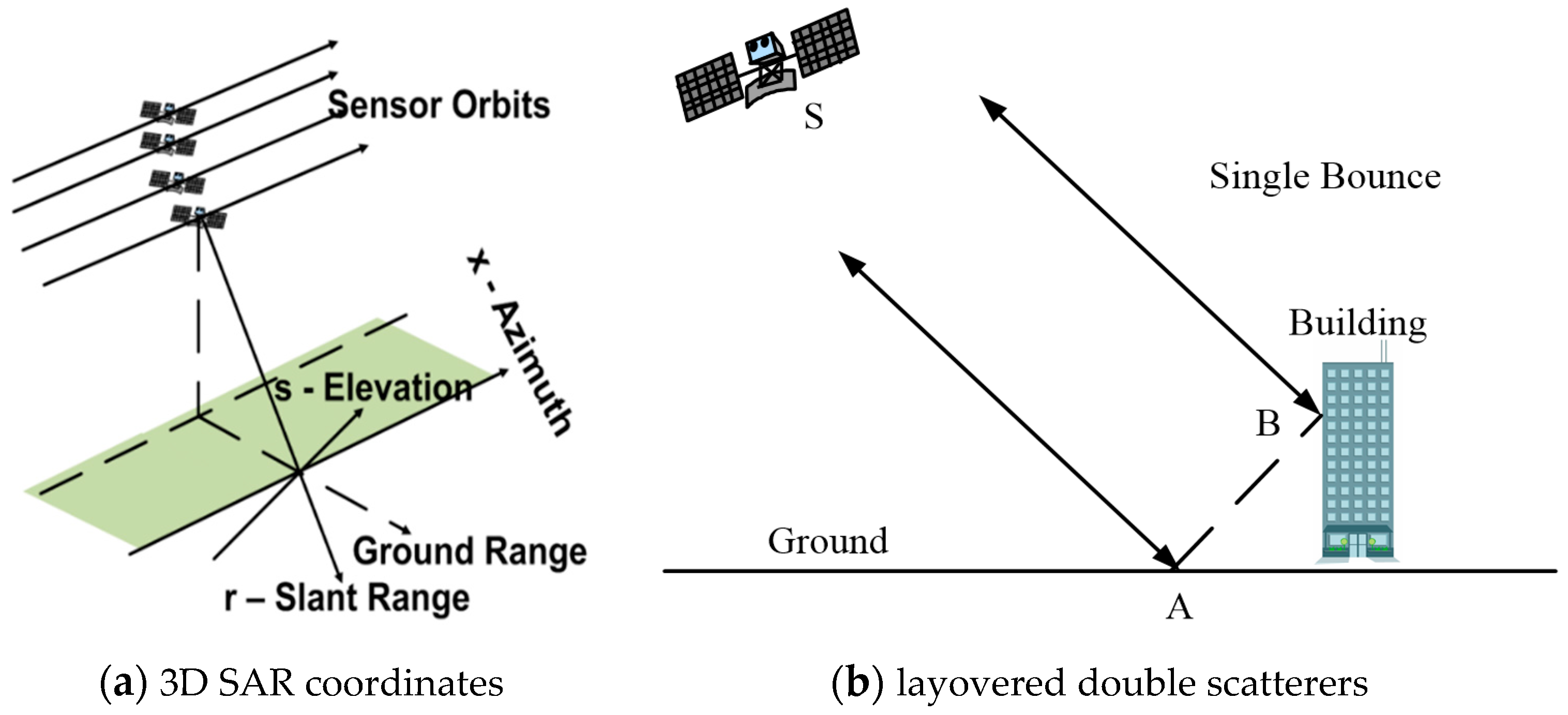
In the SAR image coordinate system, a third coordinate axis orthogonal to the azimuth–slant range (x–r) plane is defined, called elevation (s) [6] as shown in Figure 1a. A focused SAR image can be considered as a 2D projection of the 3D back-scattering scenario into the x–r plane [16]. As shown in Figure 1b, the measurement of the resolution cell contains backscattered signals from two different single-bounce scatterers (scatterers A and B), since those two single-bounce scatterers have the same slant-range distance to the sensor and will be focused into the same resolution cell [21]. With a stack of N co-registered SAR acquisitions, we are able to reconstruct the backscattering profile along the elevation direction for each resolution cell with SAR tomography. The combination of those N acquisitions forms the so-called elevation aperture.
In a stack of N co-registered SAR acquisitions, the complex value of a certain resolution cell in the nth image is considered as the integral of the real backscattering signals along elevation direction, and represented by the following Equation as
where is the elevation span, is the spatial frequency along elevation, is the backscattering magnitude along the elevation direction [16]. There are N measurements in a tomographic data stack. The continuous reflectivity model could be approximated by discretizing the function along s with a sampling frequency of L (L >> 0).
Among various tomographic reconstruction methods, Truncated Singular Value Decomposition (TSVD) is commonly used in spaceborne TomoSAR due to its good performance and computational simplicity [7]. On the other hand, Compressive Sensing (CS) based algorithms have been demonstrated to have super-resolution power. However, its high computational complexity has prevented it from being a useful tool for tomographic reconstruction of large areas on regular personal computers [22,23,24]. In our previous study, Two-step Iterative Shrinkage/Thresholding (TWIST) was proposed for TomoSAR reconstruction as a balance between TSVD and CS [29,46]. The merits of TWIST in terms of robustness, fast convergence speed, and super-resolution capability have been demonstrated by both simulations and experiments on TerraSAR-X datasets [29]. Following tomographic reconstruction, the number of scatterers, their corresponding strength/magnitude, and precise elevation positions are automatically detected from the elevation profiles by scatterers detectors. Many scatterers detectors have been proposed and assessed in literature. It is worth mentioning that with GLRT based detectors, even simple inversion scheme like beamforming can achieve a very high detection rate on single and double scatterers [19,31,32,33,34,35]. Since it is not our goal to compare different tomographic methods nor scatterers detectors, tomographic reconstruction is conducted using both TWIST and classical TSVD, combined with a common BIC-based detector in this article.
Compared to the high resolution in azimuth and range direction, the relatively poor elevation resolution does not necessarily mean that accuracy of estimated elevation is this poor. On the other hand, the estimation accuracy of individual scatterers is defined by Cramer-Rao Lower Bound (CRLB), which can be calculated with the following Equation.
where NOA is the number of acquisitions, SNR is the signal to noise ratio, and is the standard deviation of baselines [16].
2.2. Minimum Redundancy Array in SAR Tomography
The Minimum Redundancy Array (MRA), also known as Minimum Redundancy Linear Array (MRLA), was proposed in antenna array design in radio astronomy [37,47,48]. It is a subset of non-uniform linear array which provides the largest aperture for a given number of elements or uses the minimum number of elements to realize a given aperture [47,48,49]. It has been proved that the Mean Square Error (MSE) and Cramer-Rao Bound (CRB) of MRAs are the least compared with coprime and nested arrays [50,51]. A MRA is formed from a full antenna array by carefully eliminating redundant antennas while the retained elements can generate all possible antenna separation between zero and the maximum antenna length. Its merits come from the fact that it can provide the highest possible resolution with minimized redundancy [51,52]. Numerically, redundancy R is defined as the number of pairs of antennas divided by maximum spacing of the linear array. As shown in literatures [37,47], for a MRA with odd number of elements, for a MRA with even number of elements, where N is the number of elements in a linear array.
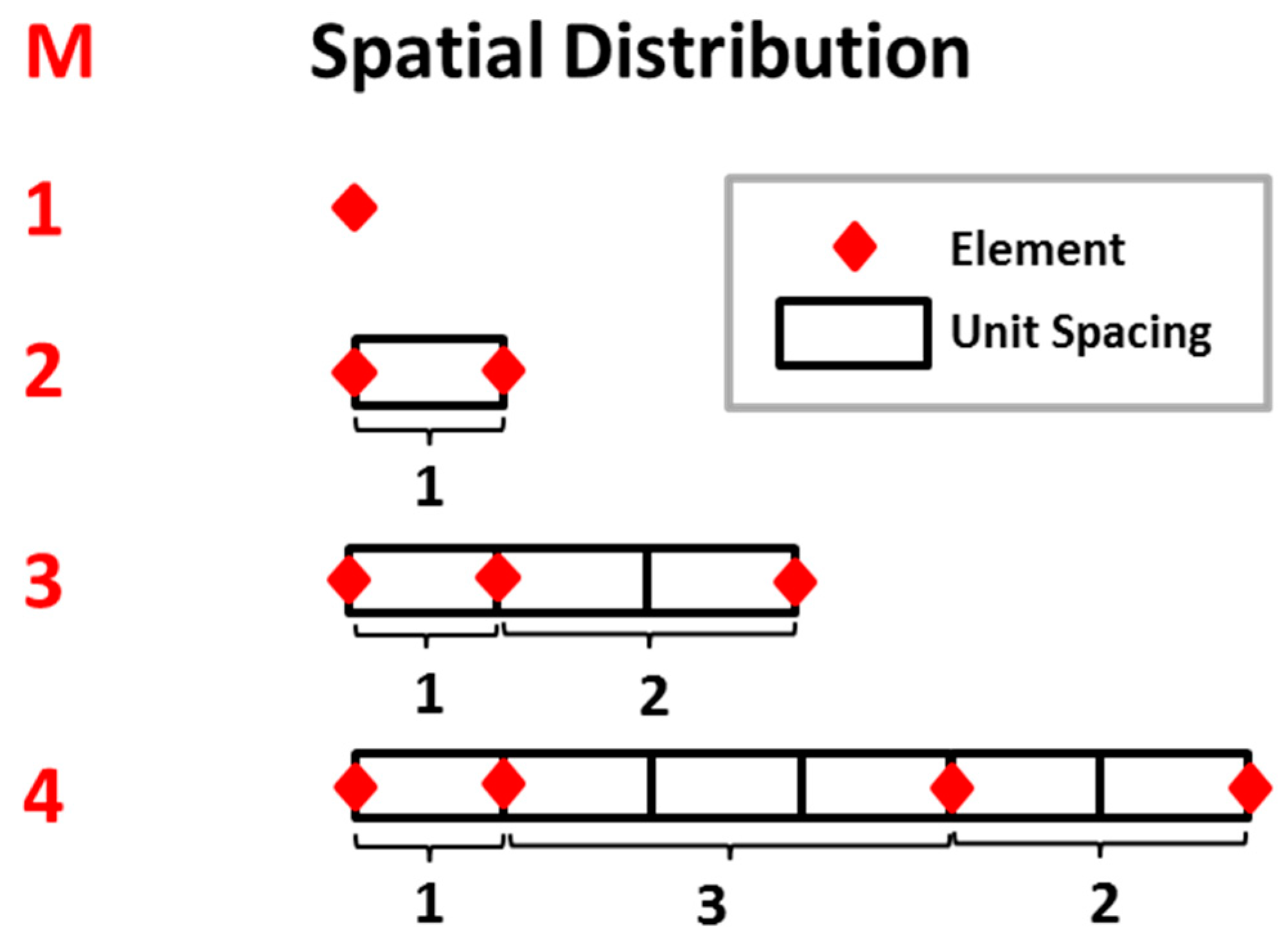
According to literatures [37,47], when the number of elements is less than 5, zero-redundancy arrays exist. In other words, there are only four zero-redundancy arrays, which have been elegantly proved in literature [52]. The four zero-redundancy arrays and their spatial distributions are shown in Figure 2. Except for the zero spacing (spatial distance) in the trivial case of single-element array, each spacing is presented only once. For example, spacing between adjacent elements are 1, 3, and 2, respectively, for the 4-element array, leading to a maximum spatial distance of 6. In other words, there is one, and only one, pair of elements separated by each multiple of the unit spacing in zero-redundancy arrays, resulting in a maximum spacing equal to the distance between the left-end and right-end elements. As shown by Figure 2, the 3-element and 4-element arrays are the only two non-uniformly distributed arrays with zero-redundancy.
For linear arrays with more than 4 elements, redundancy is always larger than 0, and there has to be some configuration of the elements which leads to minimum redundancy. However, it is not easy to find the optimum MRA configurations for a large number of elements. Wherein, the relationship between the number of MRA elements M and the array aperture N can be given by the following theorem:
For any M > 3, a set of positive integers can always be selected to satisfy the condition , and for any integer , there are always two elements with a difference of i in , and .
The problem of finding MRA for a given element number of M has been conducted by an exhaustive search, and solutions for have been given [53,54]. It has also been demonstrated that in the limit of large M, the minimum redundancy lies between 1.217 and 1.332 [54].
In urban TomoSAR, the baselines are distributed in 2-D space and can be decomposed into perpendicular and parallel baselines. What is important for TomoSAR is the so-called “elevation aperture” formed by perpendicular baselines, for the purpose of resolving multiple scatterers superimposed into one pixel along elevation direction. By ignoring the parallel baselines, the perpendicular baselines can therefore be assumed as a 1-D linear array. As shown in Equation (1), the larger the elevation aperture, the higher elevation resolution can be achieved. Similar to antenna theory, only a small elevation aperture can be formed if the baselines are uniformly distributed, and efficiency of the baseline aperture is very low. In other words, there is a high redundancy in uniform baselines configuration. Similar to the antenna theory, MRA orbits can be formed by finding a subset of M elements with baseline aperture equivalent to uniform orbits of N elements (M < N), until the redundancy reaches minimum. Therefore, the baseline distribution of MRA orbits is not strictly non-uniform, but uniform with missing orbits.
When trying to find the MRA orbits for TomoSAR, the spatial positions of SAR sensor at each revisit is considered as elements of the array, and the neighboring baselines are considered as spacing between elements. In order to keep equivalent elevation resolution, the orbits with maximum perpendicular baselines (Δb = b1 − bN) are first selected, and the smallest distance between the end-orbit and its neighbor orbit is chosen as spacing unit (u). So the initial three elements in a baseline array is configured as {.u. (Δb − u).}, where dots represent positions of the orbit and numbers refer to the spacing. Then, between spacing (Δb − u), a fourth orbit can be found located at two spacing units with reference two the end-orbits. So the baseline array becomes {.u.2u.(Δb − 3u).} or {.u.(Δb − 3u).2u.}. Following this scheme, the MRA orbits can be found iteratively. In fact, the baselines are not exactly uniformly distributed, we can only find MRA-like orbits close to the ideal MRA positions by selecting the combination with minimum standard deviation with reference to ideal MRA positions.
Let us assume the original baseline array with N elements is , and the spacing unit is selected as . So, the number of normalized baselines should be . For a given X, the normalized distributions of MRA elements have already been given in Table 1. Table 1 depicts the designed MRA orbits for and their equivalent number of uniform orbits with reference to an interval of u. If the number of MRA orbits is 10, the corresponding number of uniform orbits is 37, with 36 uniform baselines. Considering the interval of x in uniform baselines, the baseline aperture should be 36u. The positions of MRA orbits should be {0,1,3,6,13,20,27,31,35,36} multiplied by u, respectively. As shown in Table 1, the arrangement of elements for MRA is not unique. There are three different MRA orbit arrangements for M = 9, two different arrangements for M = 8, and five different MRA orbit arrangements for M = 7. These different arrangements have been studied and evaluated in [53,54]. Since it is not our goal to compare different MRA orbits, only one set of MRA orbits (highlighted in bold font in Table 1) for each M is selected for tomographic simulations in this paper.
Let us assume the optimal virtual positions of MRA baselines with M elements are , and M < N. By an exhaustive search, the real orbits close to are . Actually, there could be many choices for . The best fit of MRA-like orbits can be found by calculating the minimum Root Mean Square Error (RMSE) between and . Then the expressions in Equations (2) and (3) can be optimized as
3. Tomographic Simulations
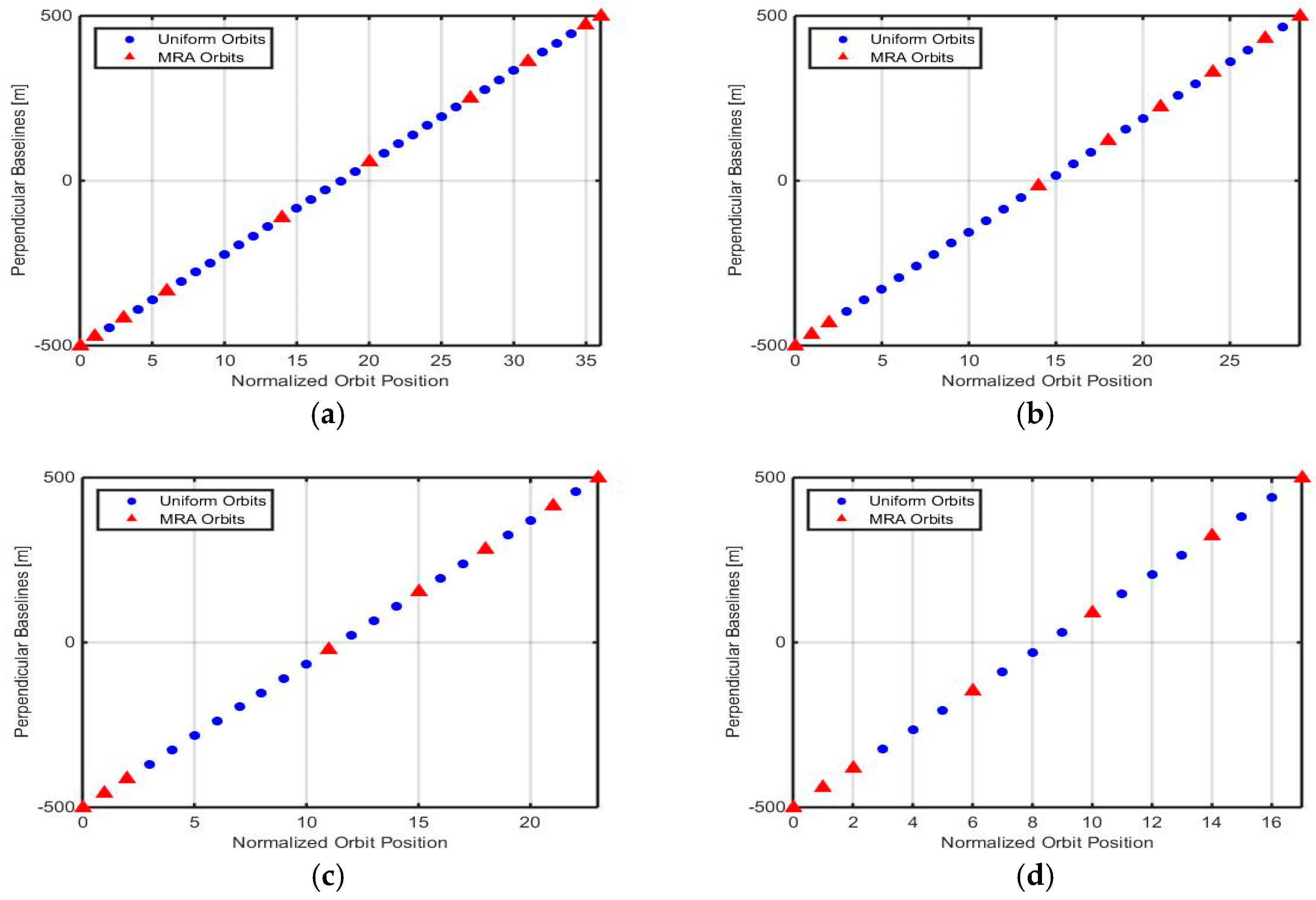
We designed four groups of uniform orbits with perpendicular baseline aperture of 1000 m in the simulation. The numbers of uniform orbits are 37, 30, 24, and 18, respectively. The baseline distributions of the four groups are shown in Figure 3, where the blue dots represent uniform orbits. Their corresponding MRA orbits are also selected following Table 1, as marked with red triangles in Figure 3. Compared to the uniform orbits, the numbers of MRA orbits are dramatically reduced.
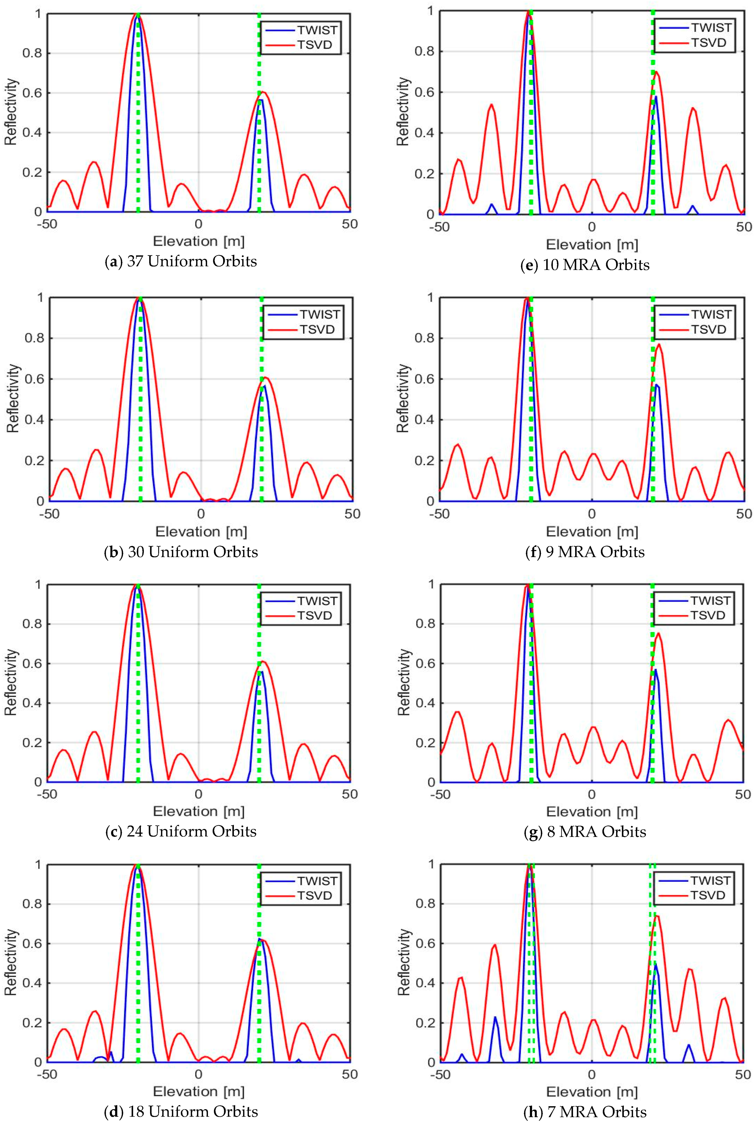
Generally, single-scatterer and double-scatterers pixels most commonly occur in layover areas of high-resolution SAR images for urban scenarios, these two cases are usually considered for TomoSAR [11]. The occurrence of more than two scatterers can increase in medium resolution SAR images like Sentinel-1, but it also depends on the geometry of the ground scene and on the elevation resolution [11]. The merit of TomoSAR is its capability in separating multiple scatterers (at least two) superimposed inside one resolution cell. Therefore, simulations on double scatterers are conducted in this section. Two scatterers located at −20 m and 20 m with normalized reflectivity of 1 and 0.6 respectively are simulated. The X-band system parameters and the four groups of orbits designed in Figure 3 are initialized for simulation. The reconstructed elevation profiles from uniform orbits in noise free case are shown in Figure 4a–d. When the orbits remain uniformly distributed with identical baseline aperture, tomographic performances of both methods are not corrupted by simply reducing the number of orbits from 37 to 18.
If the uniform orbits are replaced by their corresponding MRA orbits, TSVD suffers from dramatic increase of sidelobes, with normalized reflectivity of approximately 0.6 for the largest sidelobe, as shown in Figure 4e–h. The strong sidelobes in TSVD profiles may lead to false detection of a third scatterer. On the other hand, TWIST shows a much better resistance against sidelobes, with the largest sidelobe smaller than 0.23, see Figure 4h. By comparing the four figures in Figure 4e–h, we can tell that the normalized strengths of sidelobes in neither TSVD nor TWIST profiles are further increased when the number of MRA orbits drops from 10 to 7. This means that reducing the number of MRA orbits would also not result in a dramatic increase of sidelobes, as long as MRA orbits are used.
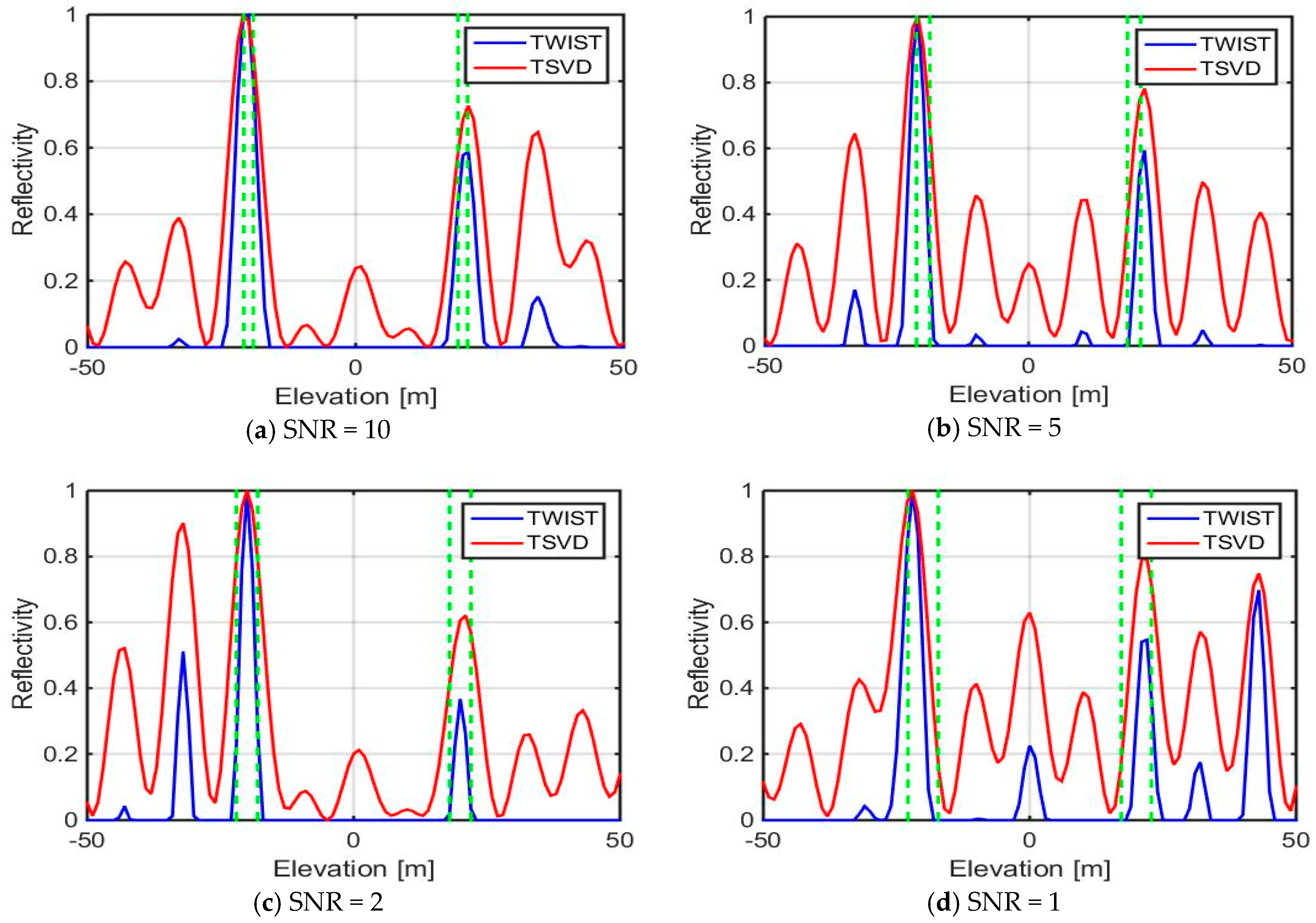
In the second simulation, white Gaussian noise at different SNR levels is added to the simulated signal. The reconstructed profiles of double scatterers from 10 MRA orbits at different SNR levels are depicted in Figure 5. As the SNR decreases, the sidelobes go up gradually for both methods, however the sidelobes in TWIST profiles are much smaller than in TSVD profiles. By comparing Figure 5 with Figure 4a, a preliminary conclusion that tomographic reconstruction can be corrupted if the SNR levels are reduced from infinite (noise free) to 1, since strong sidelobes may bury the weak scatterer’s signal or be mistaken as another scatterer, as shown in Figure 5c,d. Nevertheless, TWIST presents better resistance against noise compared with TSVD.
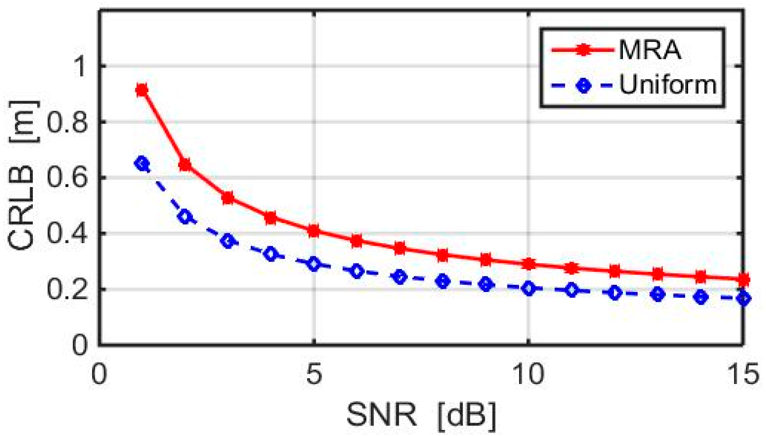
The CRLBs for MRA 10 orbits and 37 uniform orbits at different SNR levels are depicted in Figure 6. Although there is a slight drop on the CRLB using MRA orbits instead of uniform orbits, fortunately the largest decrease is within 0.3 m when SNR is 1 dB. This difference narrows quickly as the SNR increases. For SNR >= 5 dB, the difference is smaller than 0.1 m. The slight differences on CRLBs indicate that using MRA orbits instead of uniform orbits does not corrupt the estimation accuracy very much.
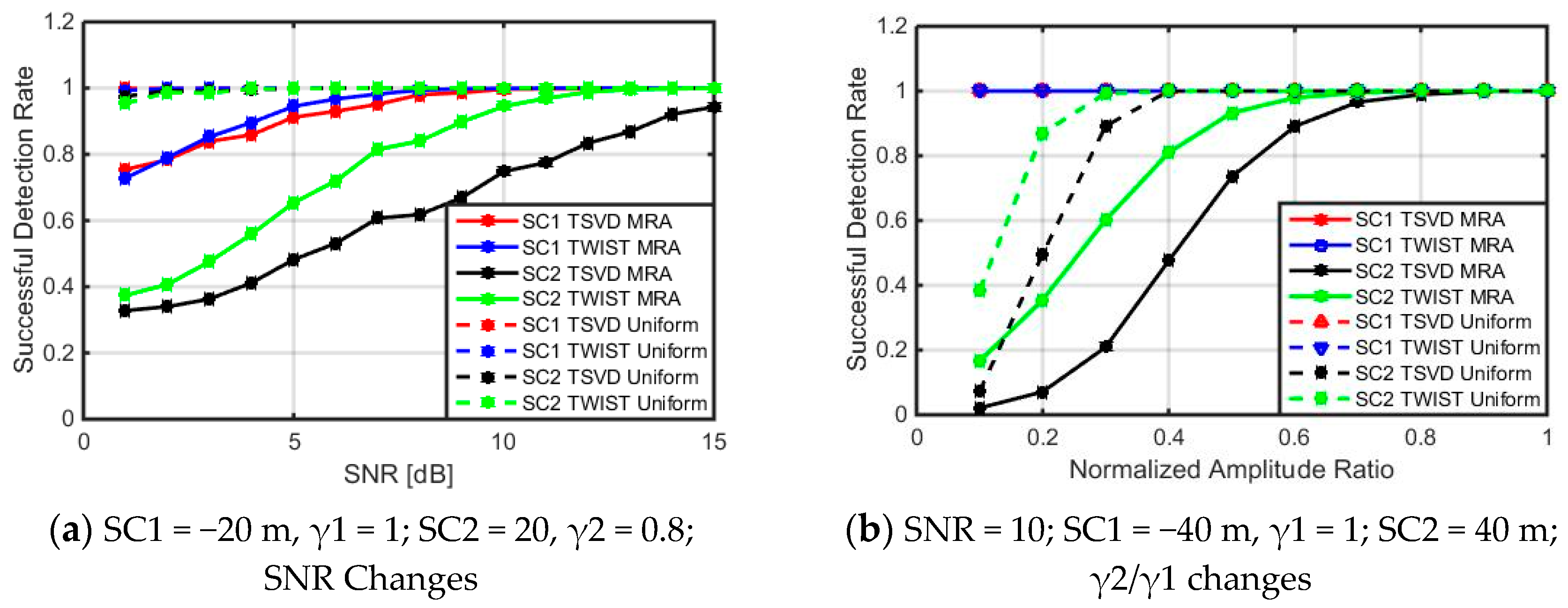
An important characteristic for evaluating the tomographic performance of MRA orbits is to analyze the successful detection rate of scatterers at different SNR levels. In order to do this, a Monte Carlo simulation on 1000 double scatters is conducted. For the purpose of avoiding influence caused by distance or amplitude ratios (γ2/γ1) between the two scatterers, identical scatterers are used for the 1000 double-scatterers pixels. A strong scatterer with normalized reflectivity of 1 is located at −40 m, and a weak scatterer with normalized reflectivity of 0.8 is located at 40 m. At each SNR level (1–15 dB), random white Gaussian noise is added to the 1000 simulated pixels. The normalized reflectivity and elevation position are automatically detected using model selection algorithm based on Bayesian Information Criterion (BIC) [32]. The successful detection rates are calculated for each scatterer at various SNR levels. A successful detection is defined when the estimated elevation is within a theoretical resolution cell centered by the real elevation position, meaning that the maximum difference between the estimated and the real elevation is smaller than half of the elevation resolution in our simulations.
The detection rates of double scatterers at different SNR levels are shown in Figure 7. As shown by the dashed lines in Figure 7a, successful detection rates of both scatterers at various SNR levels are close to 1 using uniform orbits, no matter what method (TWIST or TSVD) is used. When MRA orbits are used instead, detection rates of scatterer 1 drop slightly for both methods, with the lowest detection rate of approximately 0.7 when SNR is 1, as shown by the solid blue and red lines in Figure 7a. On the other hand, detection rates of scatterer 2 drop dramatically when MRA orbits are used, especially when TSVD method is used for tomographic reconstruction at low SNR levels, as shown by the green and black solid lines in Figure 7a. At identical SNR levels, the detection rates of scatterer 2 is generally lower than scatterer 1 using MRA orbits, this is probably caused by the reduced sampling along elevation aperture. Nevertheless, since it is useless to do tomographic analysis if there is no strong backscattering signal in a pixel (e.g., dark points on flat surface), tomographic analysis is usually conducted on pixels with strong backscattering signal (so called bright points in amplitude images). Previous study shows that SNRs of these bright points (pixels with strong backscattering signal) are generally larger than 10 dB [9]. At SNR level of 10 dB, the detection rates of both scatterers from MRA orbits would be larger than 0.95 if TWIST method is used. Therefore, the decrease of successful detection rates using MRA orbits at low SNR levels is to some extent neglectable for TWIST method, compared to the advantages in dramatically reduced number of images.
In order to analyze the successful detection rates of the weak scatterer when the amplitude ratio between two scatterers (γ2/γ1) changes, a second Monte Carlo simulation is carried out. In this simulation, a strong scatterer with normalized amplitude of 1 located at −40 m and a weak scatterer located at 40 m with normalized amplitude changes from 0.1 to 1 are simulated. Random white Gaussian noise with SNR of 10 dB is added to 1000 simulated pixels for each amplitude ratio. Both uniform orbits and MRA orbits are used for tomography. As shown by the red and blue lines in Figure 7b, detection rates of scatterer 1 is always about 1 no matter what method and what kind of orbits are used. On the other hand, detection rate of scatterer 2 increases when γ2/γ1 increases towards 1, as shown by the green and black lines in Figure 7b. The low detection rate of scatterer 2 is probably due to interference of sidelobes of scatterer 1. If the amplitude ratio is 0.4, detection rates of scatterer 2 using both methods from uniform orbits approximate to 1. On the other hand, TWIST has a detection rate of 0.82 on scatterer 2 from MRA orbits when amplitude ratio is 0.4, whereas TSVD only reaches detection rate of 0.5 on scatterer 2. As the amplitude ratio increases to 0.6, detection rate of TWIST on scatterer 2 reaches 1 from MRA orbits. However, detection rate of TSVD on scatterer 2 can only reach 1 when amplitude ratio is higher than 0.8 from MRA orbits. Therefore, using MRA orbits instead of uniform orbits does not affect the detection rate of the weak scatterer as long as the amplitude ratio is higher than 0.6 and TWIST is used for tomographic reconstruction. Unfortunately, TSVD is not able to remain equivalent detection rate from MRA orbits, with amplitude ratios smaller than 0.8.
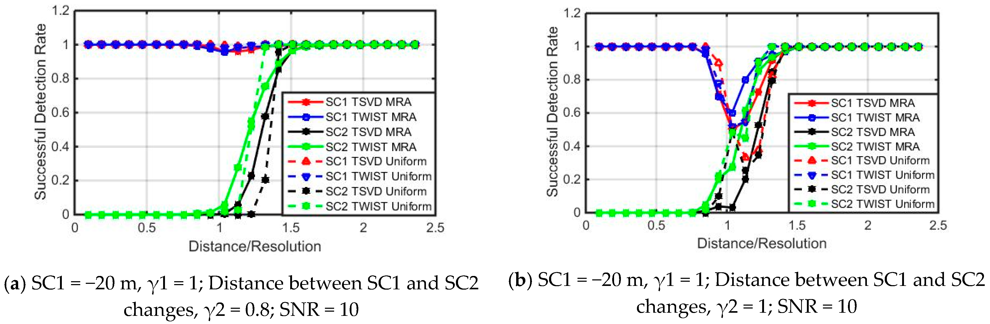
Besides SNR values and amplitude ratios, distance between double scatterers also has an impact on detection rates of both scatterers. A third Monte Carlo simulation is conducted to assess the detection rates of double scatterers when distance between scatterers change. In this Monte Carlo simulation, scatterer 1 with normalized amplitude of 1 is located at −20 m. The distance between two scatterers varies from 0 to 2.5 times of the elevation resolution. Random white Gaussian noise with SNR of 10 dB is added to 1000 simulated pixels for each distancing. Figure 8 shows the detection rates when distance between double scatterers changes. As shown in Figure 8a, when the normalized amplitude of scatterer 2 is 0.8, detection rates of scatterer 1 is generally close to 1 regardless of the distance, except for a slight drop at distances close to the theoretical elevation resolution. This slight drop is caused by interference of scatterer 2 on scatterer 1. The interference effect gets stronger when amplitude of scatterer 2 increases to 1, as shown by the sudden fluctuation on the detection rates of scatterer 1 in Figure 8b. Nevertheless, the interference effect of uniform orbits is even stronger than MRA orbits, by comparing the depth of valleys in profiles of scatterer 1, as shown by the red and blue lines in Figure 8b. This is simply because MRAs are initially designed for interference cancelation in radio astronomy.
This interference effect between two scatterers has already been discussed in literature [9] and presented in our simulations as well. If two scatterers are close enough, the estimated locations of scatterers may be shifted by the sidelobes of nearby scatterers, leading to decrease of successful detection rates, even with two scatterers further apart than the elevation resolution [16]. The elevation estimate of one scatterer is systematically biased by the sidelobes of other scatterers and vice versa, even though the SNR is high [16]. As shown by Figure 8, the interference of the strong scatterer on the weak one is much more serious than the weak one on the strong one. On one hand, the weak scatterer only causes a slight detection rate fluctuation on the strong one when their distance increases from 0 to 1.5 times of the resolution. In Figure 8a, scatterer 1 is assumed to be stronger than scatterer 2, with normalized amplitude of 1 and 0.8, respectively. The detection rate of scatterer 1 only shows a slight drop when then distance between two scatterers is smaller than 1.5 times of the resolution. If the normalized amplitude of scatterer 2 is comparable with scatterer 1, its interference on scatterer 1 gets stronger, leading to deeper fluctuation of detection rate on scatterer 1, as shown in Figure 8b. Therefore, the case of two comparable scatterers is the worst case, instead of the optimal one. If scatterer 2 gets even stronger, it will become the strong one and scatterer 1 will become the weak one. On the other hand, the strong scatterer will definitely bury the weak one if their distance is smaller than the elevation resolution. As shown by Figure 8a,b, the detection rate of scatterer 2 is 0 when distance between two scatterers is smaller than the elevation resolution. The detection rate of scatterer 2 increases gradually from 0 to 1 with distance between two scatterers increases to 1.5 times of the resolution. When the distance between two scatterers is larger than 1.5 times of the resolution, interference between two scatterers is completely gone.
As demonstrated by the above-mentioned tomographic simulations, by using MRA orbits instead of uniform orbits, the number of baselines necessary for tomographic reconstruction can be dramatically reduced, although there is a slight drop on detection rates. This problem can be somehow complemented by using TWIST method instead of spectrum estimation algorithms like TSVD. In order to further demonstrate the potential of MRA orbits in tomographic reconstruction, experimental study and discussion on COSMO-SkyMed and TerraSAR-X/TanDEM-X images are also conducted in Section 4.
4. Experimental Results with Spaceborne SAR Data
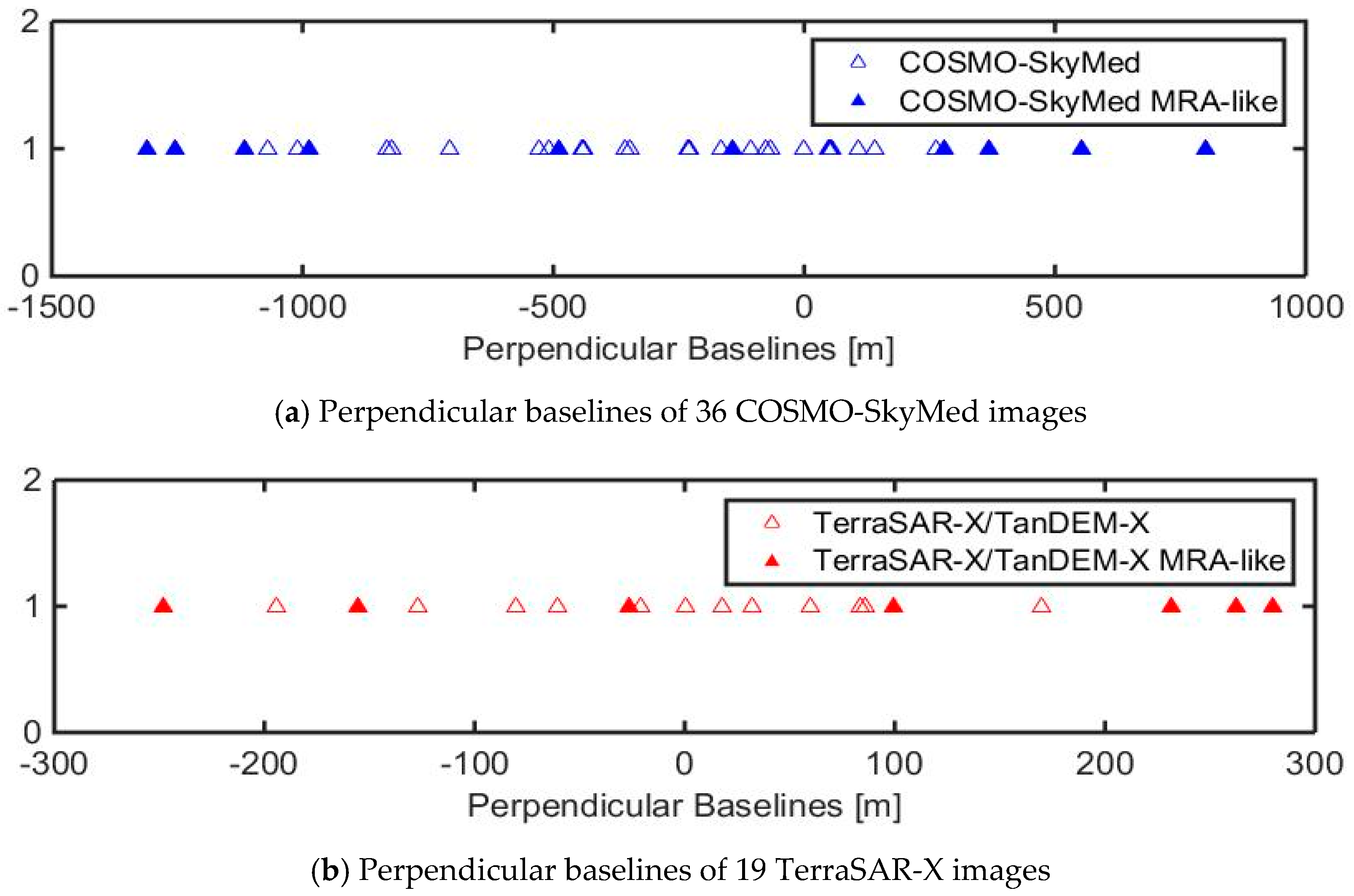
Thirty-six COSMO-SkyMed images acquired from 7 February 2015 to 10 July 2017 and nineteen TerraSAR-X/TanDEM-X images acquired from 25 August 2015 to 5 October 2016 covering Shenyang city are collected in this research. For TerraSAR-X/TanDEM-X, the satellites are orbiting the earth at the altitude of 514 km within an orbital tube of approximately 250 m radius [55,56]. On the other hand, according to the COSMO-SkyMed mission and products description, the COSMO-SkyMed satellites are running within an orbital tube that guarantees a position within +/−1000 m from a reference ground track [57]. The perpendicular baseline distributions of both stacks are depicted in Figure 9, with perpendicular baseline apertures of approximately 2110.5 m (COSMO-SkyMed) and 527.5 m (TerraSAR-X/TanDEM-X), respectively.
Since the orbits are not uniformly distributed, it is difficult to find real MRA orbits from both stacks. Instead, MRA-like orbits are selected by keeping orbits close to normalized MRA positions. As a result, ten out of thirty-six COSMO-SkyMed images and seven out of nineteen TerraSAR-X/TanDEM-X images are selected. The detailed information of both stacks is given in Table 2. According to Equation (1), the elevation resolution should be 16.7 m for TerraSAR-X/TanDEM-X and 5.1 m for COSMO-SkyMed. For comparison, two different random orbit configurations are also used for each dataset in tomographic reconstruction, respectively. The random orbits have equal number of orbits with the MRA orbits, which are ten out of thirty-six for COSMO-SkyMed dataset and seven out of nineteen for TerraSAR-X/TanDEM-X dataset, respectively. Besides, the baseline apertures for the random orbits are also identical to the MRA orbits, which are approximately 2110.5 m (COSMO-SkyMed) and 527.5 m (TerraSAR-X/TanDEM-X), respectively.
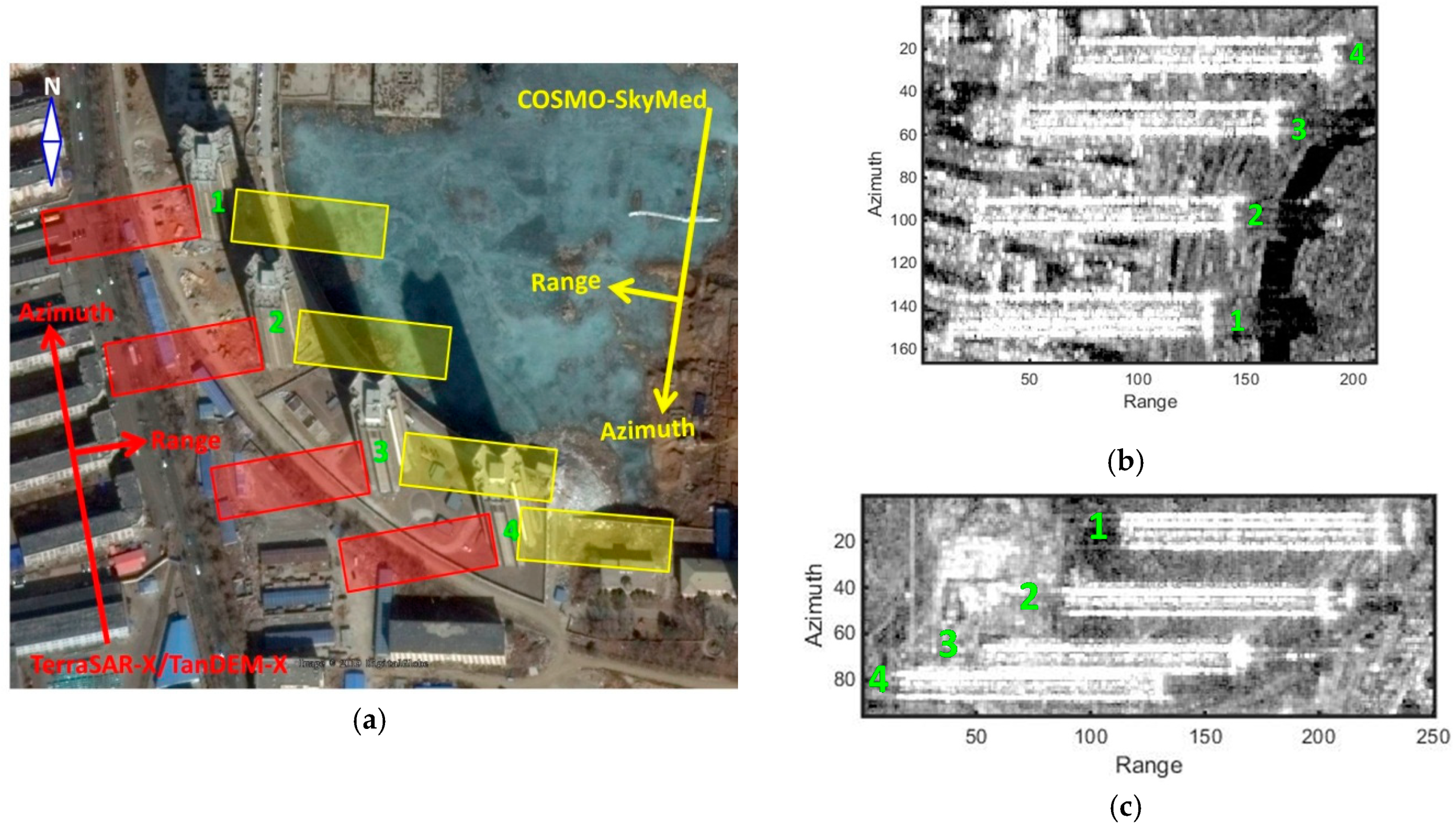
In this experiment, Longzhimeng Changyuan located in east Shenyang, with four high-rise buildings of approximately 167 m is selected as our study area. The Google earth image and SAR average amplitude images are shown in Figure 10. The COSMO-SkyMed and TerraSAR-X/TanDEM-X images are collected from descending and ascending orbits, respectively. Layover problem happens in both stacks, as highlighted with yellow and red rectangles in Figure 10a. The average amplitude images reveal that layover happens between the nearby lower buildings and the high-rise buildings in the TerraSAR-X/TanDEM-X stack, whereas layover happens between ground and the high-rise buildings in the COSMO-SkyMed stack, as shown in Figure 10b,c.
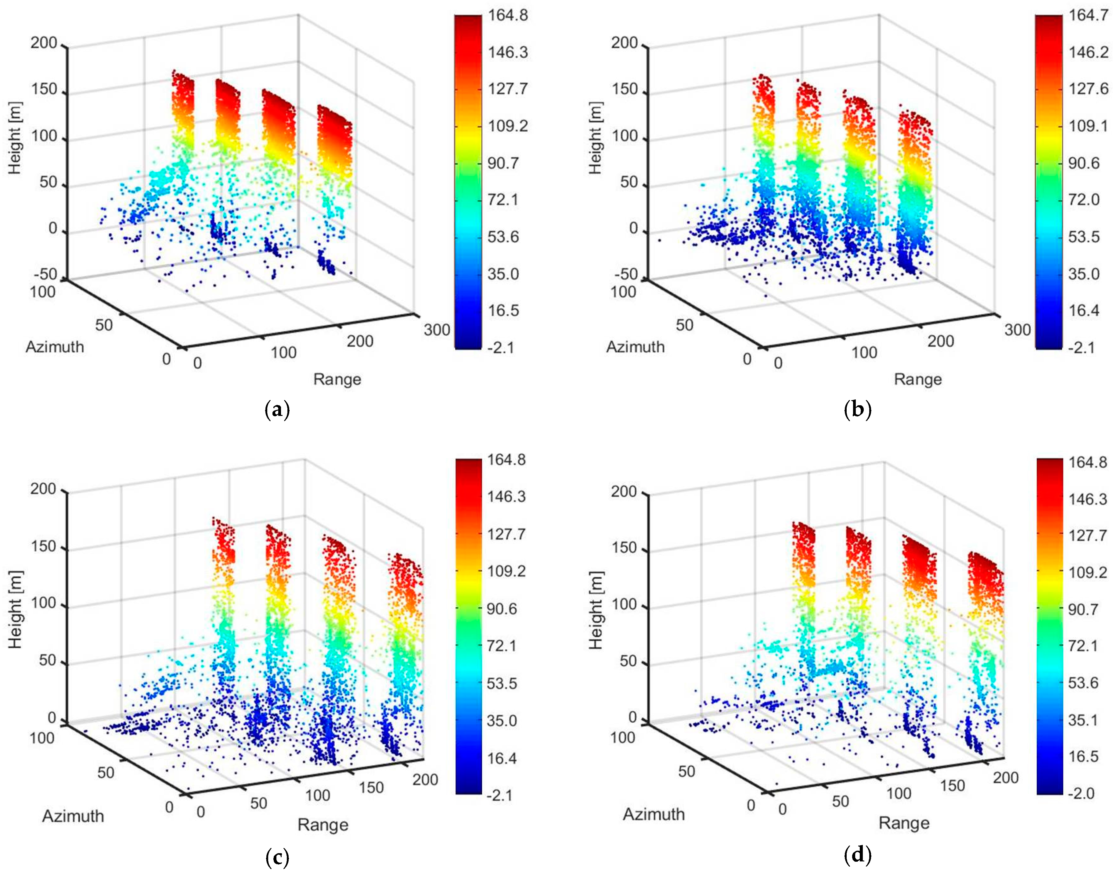
In the experimental study of spaceborne SAR data, tomographic reconstruction for Longzhimeng Changyuan is conducted using real orbits, its corresponding MRA-orbits and two different random orbit configurations, respectively. For the TerraSAR-X/TanDEM-X data stack, 4792 bright pixels are selected and reconstructed by tomographic inversion with TWIST method. As shown by the results in Figure 11a,b, we can see that the four high-rise buildings are all accurately reconstructed from real TerraSAR-X/TanDEM-X orbits and its corresponding MRA orbits. Unfortunately, the upper parts of building facades are missing in the result from random orbit configuration 1 (as shown in Figure 11c), whereas the middle parts of building facades are missing in the result from random orbit configuration 2 (as shown in Figure 11d). Therefore, by using an equally reduced number of acquisitions that do not form an MRA-like configuration, the building reconstruction is not as good.
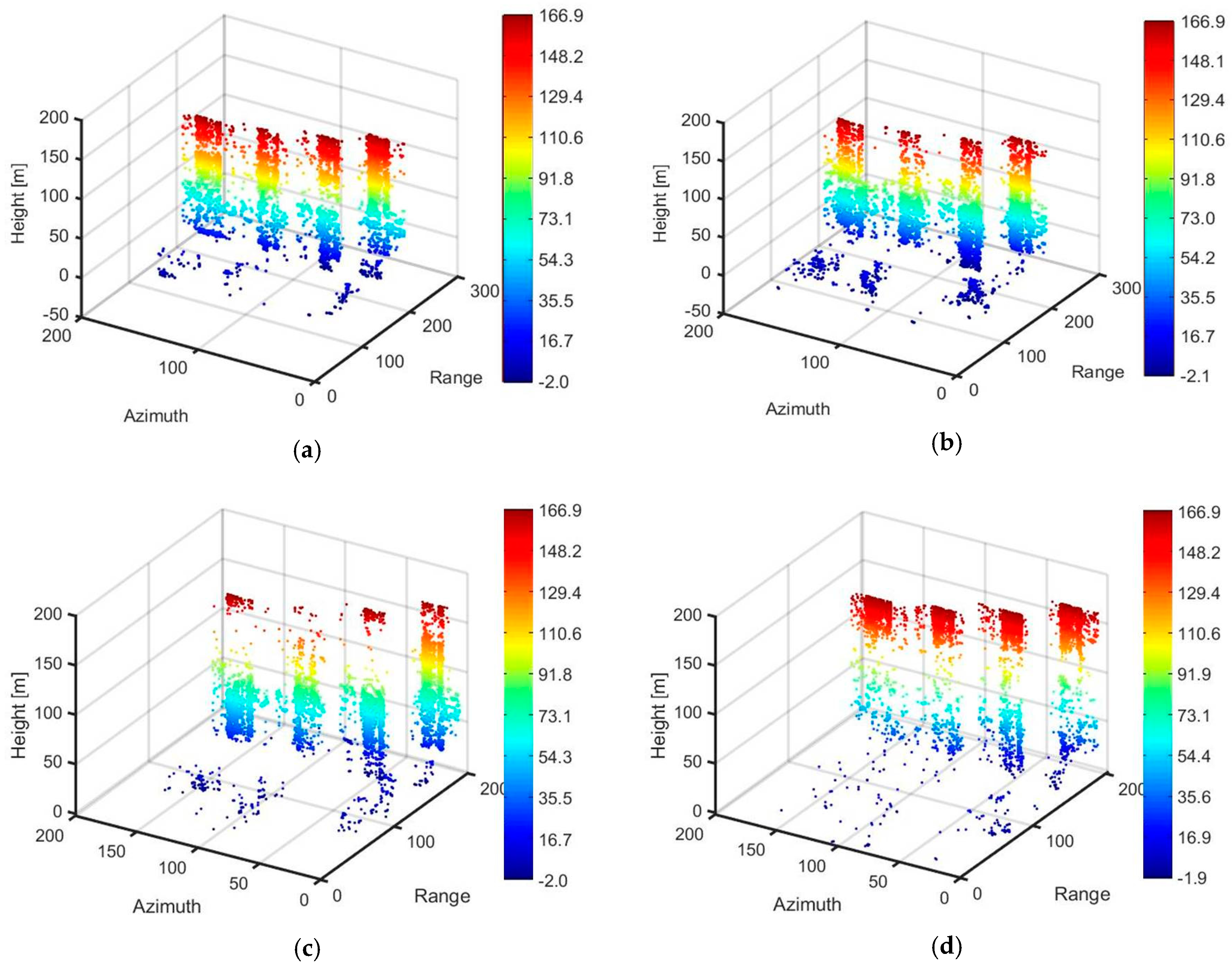
For the COSMO-SkyMed data stack, 5506 bright pixels are selected and reconstructed by TWIST method. The 3D distributions of scatterers from COSMO-SkyMed real orbits, MRA orbits, random orbit configuration 1 and random orbit configuration 2 are shown in Figure 12a–d, respectively. The heights of four high-rise buildings are all accurately reconstructed, however with lower part of building façade missing in Figure 12a,d, respectively. The whole structure of buildings is well-reconstructed from MRA orbits, as shown in Figure 12b. If the real orbits are replaced by random orbits with equal baseline aperture, the lower parts of buildings are not always precisely detected, as shown by Figure 12c,d, especially in Figure 12d. Therefore, it is possible to conduct tomographic reconstruction with robust and relatively high accuracy using dramatically reduced number of images following MRA criterion, especially when the SNR level is usually very high for many bright points in urban scenarios. As demonstrated by the results, for a fixed reduced number of acquisitions, using an MRA-like configuration is more robust than using a random configuration.
5. Discussion
In this paper, the minimum redundancy array designed for antenna formation in radio astronomy is innovatively applied to baselines optimization for the purpose of reducing number of orbits necessary for tomographic reconstruction while keeping equivalent baseline aperture. Monte Carlo simulations on double scatterers are conducted to fully evaluate the tomographic performance when MRA orbits are used instead of uniform orbits. As shown by the simulations, simply reducing the number of orbits does not corrupt tomographic performance as long as the orbits are uniformly distributed. If uniform orbits are replaced by MRA orbits, there is only a slight increase of sidelobes and slight drop on the detection rates of weak scatterers at low SNR levels using recently proposed TWIST method. However, tomographic performance using traditional spectrum estimation like TSVD suffers from dramatic corruption if MRA orbits instead of uniform orbits are used. The CRLBs calculated for simulated data indicate that using MRA orbits instead of uniform orbits has a slight drop, however within 0.1 m at SNR levels larger than 10 dB.
As shown by the experimental results on spaceborne SAR data, the merit of using MRA for baseline optimization and reduction is very well demonstrated. The experimental result from TerraSAR-X/TanDEM-X dataset shows that tomographic performance from MRA orbits is equivalent to that from original orbits. However, not so good results are derived from random orbits with identical baseline aperture and orbit numbers. As given by Figure 12, the four high-rise buildings are even better reconstructed from MRA orbits than from real COSMO-SkyMed orbits, although we do not know why for now. In order to further analyze how the non-uniform distribution of orbits affects tomographic performance, simulations and experiments on real data would be conducted in the future.
6. Conclusions
Targeting at finding out the minimum number of images necessary for tomographic reconstruction, this paper innovatively applies minimum redundancy array (MRA) for tomographic baseline array optimization. Monte Carlo simulations and experiments on spaceborne SAR data are both conducted to fully evaluate the feasibility and tomographic performance of the proposed baseline array optimization strategy. In conclusion, introducing MRA for baseline optimization in SAR tomography can benefit from the dramatic reduction of necessary orbit numbers if the recently proposed TWIST method is used for tomographic reconstruction. Although the simulation and experiments in this manuscript are carried out using spaceborne data, the outcome of this paper can also give examples for airborne TomoSAR when designing flight orbits using airborne sensors.
Author Contributions
Conceptualization, L.W.; Data curation, C.B. and C.T.; Formal analysis, L.W., Q.F. and D.Z.; Investigation, S.L. and D.Z.; Methodology, L.W.; Resources, S.L.; Software, Q.F.; Supervision, S.L.; Writing—original draft, L.W.; Writing—review & editing, L.W. and Q.F. All authors have read and agreed to the published version of the manuscript.
Funding
This research was funded by Natural Science Foundation of China (grant no. 42071453, 41601378) and the Fundamental Research Funds for the Central Universities (grant no. N2001027). The APC was funded by the Fundamental Research Funds for the Central Universities no. N2001027.
Acknowledgments
The COSMO-SkyMed data was provided by ASI via the ASI-ESA Dragon4 Project ID. 32365_4 and ASI-ESA Dragon5 Project ID. 58029. The TerraSAR-X/TanDEM-X data was provided by Airbus Defense and Space. The authors would like to thank the editors and anonymous reviewers for their constructive comments and efforts spent on this manuscript.
Conflicts of Interest
The authors declare no conflict of interest.
References
- Gini, F.; Lombardini, F.; Montanari, M. Layover solution in multibaseline SAR interferometry. IEEE Trans. Aerosp. Electron. Syst. 2002, 38, 1344–1356. [Google Scholar] [CrossRef]
- Fornaro, G.; Lombardini, F.; Pauciullo, A.; Reale, D.; Viviani, F. Tomographic processing of interferometric SAR data: Developments, applications, and future research perspectives. IEEE Sign. Proc. Mag. 2014, 31, 41–50. [Google Scholar] [CrossRef]
- Zhu, X. A review of ten-year advances of multi-baseline SAR interferometry using TerraSAR-X data. Remote Sens. 2018, 10, 1–32. [Google Scholar] [CrossRef]
- Chan, C.; Farhat, N.H. Frequency swept tomographic imaging of three-dimensional perfectly conducting objects. IEEE Trans. Antennas Propag. 1981, 29, 312–319. [Google Scholar] [CrossRef]
- Reigber, A.; Moreira, A. First demonstration of airborne SAR tomography using multibaseline L-band data. IEEE Trans. Geosci. Remote Sens. 2000, 38, 2142–2152. [Google Scholar] [CrossRef]
- Fornaro, G.; Serafino, F.; Soldovieri, F. Three-dimensional focusing with multipass SAR data. IEEE Trans. Geosci. Remote Sens. 2003, 41, 507–517. [Google Scholar] [CrossRef]
- Fornaro, G.; Serafino, F.; Lombardini, F. Three-dimensional multi-pass SAR focusing: Experiments with long-term spaceborne data. IEEE Trans. Geosci. Remote Sens. 2005, 43, 702–714. [Google Scholar] [CrossRef]
- Fornaro, G.; Serafino, F. Imaging of single and double scatterers in urban areas via SAR tomography. IEEE Trans. Geosci. Remote Sens. 2006, 44, 3497–3505. [Google Scholar] [CrossRef]
- Reale, D.; Fornaro, G.; Pauciullo, A.; Zhu, X.; Bamler, R. Tomographic imaging and monitoring of buildings with very high resolution SAR data. IEEE Geosci. Remote Sens. Lett. 2011, 8, 661–665. [Google Scholar] [CrossRef] [Green Version]
- Fornaro, G.; Pauciullo, A.; Reale, D.; Verde, S. Multilook SAR tomography for 3-D reconstruction and monitoring of single structures applied to COSMO-SKYMED data. IEEE J. Sel. Top. Appl. Earth Obs. Remote Sens. 2014, 7, 2776–2785. [Google Scholar] [CrossRef]
- Budillon, A.; Crosetto, M.; Johnsy, A.C.; Monserrat, O.; Krishnakumar, V.; Schirinzi, G. Comparison of persistent scatterer interferometry and SAR tomography using Sentinel-1 in urban environment. Remote Sens. 2018, 10, 1986. [Google Scholar] [CrossRef] [Green Version]
- Budillon, A.; Johnsy, A.C.; Schirinzi, G. Urban tomographic imaging using polarimetric SAR data. Remote Sens. 2019, 11, 132. [Google Scholar] [CrossRef] [Green Version]
- Lu, H.; Zhang, H.; Deng, Y.; Wang, J.; Yu, W. Building 3-D reconstruction with a small data stack using SAR tomography. IEEE J. Sel. Top. Appl. Earth Obs. Remote Sens. 2020, 13, 2461–2474. [Google Scholar] [CrossRef]
- Lombardini, F.; Cai, F.; Pasculli, D. Spaceborne 3-D SAR tomography for analyzing garbled urban scenarios: Single-look superresolution advances and experiments. IEEE J. Sel. Top. Appl. Earth Obs. Remote Sens. 2013, 6, 960–968. [Google Scholar] [CrossRef]
- Montazeri, S.; Zhu, X.; Member, S.; Eineder, M.; Bamler, R. Three-dimensional deformation monitoring of urban infrastructure by tomographic SAR using multitrack TerraSAR-X data stacks. IEEE Trans. Geosci. Remote Sens. 2016, 54, 6868–6878. [Google Scholar] [CrossRef]
- Zhu, X.; Bamler, R. Very high resolution spaceborne SAR tomography in urban environment. IEEE Trans. Geosci. Remote Sens. 2010, 48, 4296–4308. [Google Scholar] [CrossRef] [Green Version]
- Zhu, X.; Montazeri, S.; Gisinger, C.; Hanssen, R.; Bamler, R. Geodetic SAR tomography. IEEE Trans. Geosci. Remote Sens. 2016, 54, 18–35. [Google Scholar] [CrossRef] [Green Version]
- Ge, N.; Gonzalez, F.R.; Wang, Y.; Shi, Y.; Zhu, X.X. Spaceborne staring spotlight SAR tomography-a first demonstration with TerraSAR-X. IEEE J. Sel. Top. Appl. Earth Obs. Remote Sens. 2018, 11, 3743–3756. [Google Scholar] [CrossRef] [Green Version]
- Zhu, X. Spectral Estimation for Synthetic Aperture Radar Tomography. Master’s Thesis, Technical University of Munich, Munich, Germany, 2008; pp. 1–75. [Google Scholar]
- Stoica, P.; Moses, R. Spectral Analysis of Signals; Prentice-Hall: Upper Saddle River, NJ, USA, 2005. [Google Scholar]
- Wei, L.; Balz, T.; Liao, M.; Zhang, L. TerraSAR-X stripMap data interpretation of complex urban scenarios with 3D SAR tomography. J. Sens. 2014, 2014, 386753. [Google Scholar] [CrossRef]
- Candès, E.J. Compressive sampling. In Proceedings of the International Congress of Mathematicians, Madrid, Spain, 22–30 August 2006; pp. 1–20. [Google Scholar]
- Donoho, D. Compressed sensing. IEEE Trans. Inf. Theor. 2006, 52, 1289–1306. [Google Scholar] [CrossRef]
- Zhu, X.; Bamler, R. Tomographic SAR inversion by L1 norm regularization–the compressive sensing approach. IEEE Trans. Geosci. Remote Sens. 2010, 48, 1–8. [Google Scholar] [CrossRef] [Green Version]
- Budillon, A.; Evangelista, A.; Schirinzi, G. Three-dimensional SAR focusing from multipass signals using compressive sampling. IEEE Trans. Geosci. Remote Sens. 2011, 49, 488–499. [Google Scholar] [CrossRef]
- Zhu, X.; Bamler, R. Super-resolution power and robustness of compressive sensing for spectral estimation with application to spaceborne tomographic SAR. IEEE Trans. Geosci. Remote Sens. 2012, 50, 247–258. [Google Scholar] [CrossRef]
- Zhu, X.; Bamler, R. Demonstration of super-resolution for tomographic SAR imaging in urban environment. IEEE Trans. Geosci. Remote Sens. 2012, 50, 3150–3157. [Google Scholar] [CrossRef] [Green Version]
- Zhu, X.; Ge, N.; Shahzad, M. Joint sparsity in SAR tomography for urban mapping. IEEE J. Sel. Top. Sign. Process. 2015, 9, 1498–1509. [Google Scholar] [CrossRef] [Green Version]
- Wei, L.; Balz, T.; Zhang, L.; Liao, M. A novel fast approach for SAR tomography: Two-step iterative shrinkage/thresholding. IEEE Geosci. Remote Sens. Lett. 2015, 12, 1377–1381. [Google Scholar]
- Zhu, X.; Dong, Z.; Yu, A.; Wu, M.; Li, D.; Zhang, Y. New approaches for robust and efficient detection of persistent scatterers in SAR tomography. Remote Sens. 2019, 11, 356. [Google Scholar] [CrossRef] [Green Version]
- Ferretti, A.; Bianchi, M.; Prati, C.; Rocca, F. Higher order permanent scatterers analysis. EURASIP 2004, 1–30. [Google Scholar] [CrossRef] [Green Version]
- Schwarz, G. Estimating the dimension of a model. Ann. Stat. 1978, 6, 461–464. [Google Scholar] [CrossRef]
- De Maio, A.; Fornaro, G.; Pauciullo, A. Detection of single scatterers in multidimensional SAR imaging. IEEE Trans. Geosci. Remote Sens. 2009, 47, 2284–2297. [Google Scholar] [CrossRef]
- Pauciullo, A.; Reale, D.; De Maio, A.; Fornaro, G. Detection of double scatterers in SAR tomography. IEEE Trans. Geosci. Remote Sens. 2012, 50, 3567–3586. [Google Scholar] [CrossRef]
- Budillon, A.; Schirinzi, G. GLRT based on support estimation for multiple scatterers detection in SAR tomography. IEEE J. Sel. Top. Appl. Earth Obs. Remote Sens. 2016, 9, 1086–1094. [Google Scholar] [CrossRef]
- Nannini, M.; Scheiber, R.; Moreira, A. Estimation of the minimum number of tracks for SAR tomography. IEEE Trans. Geosci. Remote Sens. 2009, 47, 531–543. [Google Scholar] [CrossRef]
- Moffet, A.T. Minimum-redundancy linear arrays. IEEE Trans. Antenne Propag. 1968, 16, 172–175. [Google Scholar] [CrossRef] [Green Version]
- Chambers, C.; Tozer, T.C.; Sharman, K.C. Temporal and spatial sampling influence on the estimates of superimposed narrowband signals: When less can mean more. IEEE Trans. Signal Proc. 1996, 44, 3085–3098. [Google Scholar] [CrossRef]
- Abramovich, Y.I.; Spencer, N.K. Gorokhov A Y. Positive-definite Toeplitz completion in DOA estimation for nonuniform linear antenna arrays. IEEE Trans. Signal Proc. 1999, 47, 1502–1521. [Google Scholar] [CrossRef]
- Ahmad, A.; Behera, A.K.; Mandal, S.K. Artificial bee colony algorithm to reduce the side lobe level of uniformly excited linear antenna arrays through optimized element spacing. In Proceedings of the IEEE Conference on Information & Communication Technologies 2013 (ICT 2013), Thuckalay, India, 11–13 April 2013; pp. 1029–1032. [Google Scholar]
- Yang, S.H.; Kiang, J.F. Optimization of asymmetrical difference pattern with memetic algorithm. IEEE Trans. Antennas Propag. 2014, 62, 2297–2302. [Google Scholar] [CrossRef]
- Joshi, P.; Dubey, R. Optimization of linear antenna array using genetic algorithm for reduction in side lobs levels and improving directivity based on modulating parameter M. Optimization 2013, 1, 1475–1482. [Google Scholar]
- Lu, H.; Liu, H.; Luo, T.; Suo, Z.; Jiu, B.; Bao, Z. Optimal baseline design for SAR tomography system. J. Electron. Inform. Technol. 2015, 37, 919–925. (In Chinese) [Google Scholar]
- Bi, H.; Liu, J.; Zhang, B.; Hong, W. Baseline distribution optimization and missing data completion in wavelet-based CS-TomoSAR. Sci. China Inf. Sci. 2018, 61, 1–9. [Google Scholar] [CrossRef]
- Zhao, J.; Yu, A.; Zhang, Y.; Zhu, X.; Dong, Z. Spatial baseline optimization for spaceborne multistatic SAR tomography systems. Sensors 2019, 19, 2106. [Google Scholar] [CrossRef] [PubMed] [Green Version]
- Bioucas-Dias, J.M.; Figueiredo, M.A.T. A new TwIST: Two-step iterative shrinkage/thresholding algorithms for image restoration. IEEE Trans. Image Process. 2007, 16, 2992–3004. [Google Scholar] [CrossRef] [PubMed] [Green Version]
- Ishiguro, M. Minimum redundancy linear arrays for a large number of antennas. Radio Sci. 1980, 15, 1163–1170. [Google Scholar] [CrossRef]
- Bracewell, R.N. Radio astronomy techniques. In Handbuch der Physik; Springer: Berlin/Heidelberg, Germany, 1962; Volume 54, pp. 42–129. [Google Scholar]
- Pearson, D.; Pillai, S.U.; Lee, Y. An algorithm for near optimal placement of sensor elements. IEEE Trans. Inf. Theor. 1990, 36, 1280–1284. [Google Scholar] [CrossRef]
- Wang, M.; Nehorai, A. Coarrays, music, and the Cramér-Rao bound. IEEE Trans. Signal Proc. 2017, 65, 933–946. [Google Scholar] [CrossRef] [Green Version]
- Liu, C.-L.; Vaidyanathan, P.P. Cramér–Rao bounds for coprime and other sparse arrays, which find more sources than sensors. Digit. Sign. Process. 2017, 61, 43–61. [Google Scholar] [CrossRef] [Green Version]
- Patwari, A.; Ramachandra Reddy, G. A conceptual framework for the use of minimum redundancy linear arrays and flexible arrays in future smartphones. Int. J. Antennas Propag. 2018, 2018, 1–12. [Google Scholar] [CrossRef]
- Leech, J. On the representation of 1, 2, …, n by differences. J. London Math. Soc. 1956, 31, 160–169. [Google Scholar] [CrossRef]
- Panayirci, E.; Chen, W.L. Minimum redundancy array structure for interference cancellation. Sign. Process. 1995, 42, 319–334. [Google Scholar] [CrossRef]
- Werninghaus, R.; Buckreuss, S. The TerraSAR-X mission and system design. IEEE Trans. Geosci. Remote Sens. 2010, 48, 606–614. [Google Scholar] [CrossRef] [Green Version]
- Kahle, R.; Kazeminejad, B.; Kirschner, M.; Yoon, Y.; Kiehling, R.; D’Amico, S. First in-orbit experience of TerraSAR-X flight dynamics operations. In Proceedings of the 20th International Symposium on Space Flight Dynamics, Annapolis, MD, USA, 24–28 September 2007. [Google Scholar]
- Fiorentino, C.; Virelli, M. COSMO-SkyMed Mission and Products Description; Agenzia Spaziale Italiana ASI: Rome, Italy, 2019; p. 151.
Figure 1.
3D SAR coordinate system (a) and typical layover effect of double single-bounce scatterers in urban SAR images (b).
Figure 1.
3D SAR coordinate system (a) and typical layover effect of double single-bounce scatterers in urban SAR images (b).

Figure 2.
The four zero-redundancy linear arrays and their spatial distribution, where red diamonds represent spatial positions of elements, white bars represent spacing (spatial distance) between adjacent elements.
Figure 2.
The four zero-redundancy linear arrays and their spatial distribution, where red diamonds represent spatial positions of elements, white bars represent spacing (spatial distance) between adjacent elements.

Figure 3.
The simulated uniform orbits and their corresponding MRA orbits: (a) 10 MRA out of 37 uniform orbits; (b) 9 MRA out of 30 uniform orbits; (c) 8 MRA out of 24 uniform orbits; (d) 7 MRA out of 18 uniform orbits.
Figure 3.
The simulated uniform orbits and their corresponding MRA orbits: (a) 10 MRA out of 37 uniform orbits; (b) 9 MRA out of 30 uniform orbits; (c) 8 MRA out of 24 uniform orbits; (d) 7 MRA out of 18 uniform orbits.

Figure 4.
Tomographic performance of TWIST and TSVD on double scatters using uniform orbits (a–d) and MRA orbits (e–h) in noise free case.
Figure 4.
Tomographic performance of TWIST and TSVD on double scatters using uniform orbits (a–d) and MRA orbits (e–h) in noise free case.

Figure 5.
Tomographic performance of TWIST and TSVD on double scatters at different SNR levels when 10 MRA orbits are used.
Figure 5.
Tomographic performance of TWIST and TSVD on double scatters at different SNR levels when 10 MRA orbits are used.

Figure 6.
Cramer-Rao Lower Bound (CRLB) at different SNR levels.

Figure 7.
Successful detection rate of 1000 simulated double-scatterer pixels at different SNR levels (a) and normalized amplitude ratios (γ2/γ1) (b), where SC abbreviates from scatterer and γ is the normalized reflectivity (amplitude).
Figure 7.
Successful detection rate of 1000 simulated double-scatterer pixels at different SNR levels (a) and normalized amplitude ratios (γ2/γ1) (b), where SC abbreviates from scatterer and γ is the normalized reflectivity (amplitude).

Figure 8.
Successful detection rates of double scatterers when distance between both scatterers changes, where SC abbreviates from scatterer, γ is the normalized reflectivity (amplitude).
Figure 8.
Successful detection rates of double scatterers when distance between both scatterers changes, where SC abbreviates from scatterer, γ is the normalized reflectivity (amplitude).

Figure 9.
Perpendicular baselines of COSMO-SkyMed and TerraSAR-X/TanDEM-X images.

Figure 10.
Remote sensing images of the Longzhimeng Changyuan study area: (a) Google Earth image; (b) average amplitude of the TerraSAR-X/TanDEM-X images; (c) average amplitude of the COSMO-SkyMed images.
Figure 10.
Remote sensing images of the Longzhimeng Changyuan study area: (a) Google Earth image; (b) average amplitude of the TerraSAR-X/TanDEM-X images; (c) average amplitude of the COSMO-SkyMed images.

Figure 11.
3D distribution of scatters reconstructed by TWIST for Longzhimeng Changyuan using TerraSAR-X/TanDEM-X orbits (a) the corresponding MRA orbits (b) random orbit configuration 1 (c) and random orbit configuration 2 (d), respectively.
Figure 11.
3D distribution of scatters reconstructed by TWIST for Longzhimeng Changyuan using TerraSAR-X/TanDEM-X orbits (a) the corresponding MRA orbits (b) random orbit configuration 1 (c) and random orbit configuration 2 (d), respectively.

Figure 12.
3D distribution of scatters reconstructed by TWIST for Longzhimeng Changyuan using COSMO-SkyMed orbits (a) the corresponding MRA orbits (b) random orbit configuration 1 (c) and random orbit configuration 2 (d), respectively.
Figure 12.
3D distribution of scatters reconstructed by TWIST for Longzhimeng Changyuan using COSMO-SkyMed orbits (a) the corresponding MRA orbits (b) random orbit configuration 1 (c) and random orbit configuration 2 (d), respectively.


Table 1.
Normalized distributions of minimum redundancy array (MRA) orbits.
| M | N | Normalized Positions of MRA Orbits with Reference to an Interval of u |
|---|---|---|
| 10 | 37 | 0,1,3,6,13,20,27,31,35,36 |
| 9 9 9 | 30 30 30 | 0,1,2,14,18,21,24,27,29 0,1,3,6, 13,20,24,28,29 0,1,4,10,16,22,24,27,29 |
| 8 8 | 24 24 | 0,1,2,11,15,18,21,23 0,1,4,10,16,18,21,23 |
| 7 7 7 7 7 | 18 18 18 18 18 | 0,1,2,3,8,13,17 0,1,2,6,10,14,17 0,1,2,8,12,14,17 0,1,2,8,12,15,17 0,1,8,11,13,15,17 |
M represents number of MRA orbits; N represents number of uniform orbits; N − 1 represents the number of uniform baselines.
Table 2.
Parameters of the data stacks.
| Sensor | TerraSAR-X/TanDEM-X | COSMO-SkyMed |
|---|---|---|
| Number of Images | 19 | 36 |
| Orbit | Ascending | Descending |
| Work Mode | StripMap | StripMap |
| Altitude | 514 km | 619.6 km |
| Azimuth Resolution | 3.3 m | 3.0 |
| Slant Range Resolution | 1.2 m | 1.3 m |
| Incidence Angle () | 24.3 | 25.1 |
| Baseline Aperture () | 527.5 m | 2110.5 m |
| Elevation Resolution () | 16.7 m | 5.1 m |
© 2020 by the authors. Licensee MDPI, Basel, Switzerland. This article is an open access article distributed under the terms and conditions of the Creative Commons Attribution (CC BY) license (http://creativecommons.org/licenses/by/4.0/).
Share and Cite
MDPI and ACS Style
Wei, L.; Feng, Q.; Liu, S.; Bignami, C.; Tolomei, C.; Zhao, D. Minimum Redundancy Array—A Baseline Optimization Strategy for Urban SAR Tomography. Remote Sens. 2020, 12, 3100. https://doi.org/10.3390/rs12183100
AMA Style
Wei L, Feng Q, Liu S, Bignami C, Tolomei C, Zhao D. Minimum Redundancy Array—A Baseline Optimization Strategy for Urban SAR Tomography. Remote Sensing. 2020; 12(18):3100. https://doi.org/10.3390/rs12183100
Chicago/Turabian StyleWei, Lianhuan, Qiuyue Feng, Shanjun Liu, Christian Bignami, Cristiano Tolomei, and Dong Zhao. 2020. "Minimum Redundancy Array—A Baseline Optimization Strategy for Urban SAR Tomography" Remote Sensing 12, no. 18: 3100. https://doi.org/10.3390/rs12183100
Note that from the first issue of 2016, this journal uses article numbers instead of page numbers. See further details here.