Disentangled Autoencoder for Cross-Stain Feature Extraction in Pathology Image Analysis


1
RECETOX, Masaryk University, 62500 Brno, Czech Republic
2
Chair for Computer Aided Medical Procedures, Technical University of Munich, 80333 Munich, Germany
*
Author to whom correspondence should be addressed.
Appl. Sci. 2020, 10(18), 6427; https://doi.org/10.3390/app10186427
Submission received: 3 July 2020
/
Revised: 8 September 2020
/
Accepted: 11 September 2020
/
Published: 15 September 2020
(This article belongs to the Special Issue Recent Advances in Biomedical Image Processing)
Abstract
:Featured Application
The method described can be applied for stain-independent pathology image registration and content summarization.
Abstract
A novel deep autoencoder architecture is proposed for the analysis of histopathology images. Its purpose is to produce a disentangled latent representation in which the structure and colour information are confined to different subspaces so that stain-independent models may be learned. For this, we introduce two constraints on the representation which are implemented as a classifier and an adversarial discriminator. We show how they can be used for learning a latent representation across haematoxylin-eosin and a number of immune stains. Finally, we demonstrate the utility of the proposed representation in the context of matching image patches for registration applications and for learning a bag of visual words for whole slide image summarization.
1. Introduction
Digital pathology underwent a significant transformation during the last years, to become a key tool in modern clinical practice and research. This was facilitated by the developments both in hardware, with cheaper and faster computers and storage, the availability of more powerful graphics processing units (GPUs) with larger memory, faster slide scanners, etc., and computational methods, with deep learning approaches being the most prominent example. Having faster and more performant pathology slide scanners, enables almost mass-production of digital slide archives and puts high pressure on the computational infrastructure. For example, a single whole slide image (WSI) of a tissue sample scanned at magnification easily contains multi-channel pixels, describing highly complex multi-scale structures. Clearly, there is a need for highly performant image analysis methods able to detect, extract, measure and summarize these structures. For a detailed review of the current challenges and trends in digital pathology, see [1,2].
Immunohistochemistry (IHC) is a method for visualizing at light microscopy level the spatial distribution of targets (antigens) of interest by exploiting the specificity of antibody binding with its antigen. Routine IHC is limited in the number of antibodies (colours) that can be used in a single tissue section meaning that for studying the (co-)distribution of several targets one needs several consecutive sections. More recently, a number of protocols (e.g., stain multiplexing) allow the use of several antibodies for visualizing multiple targets at the same time. Here, we are interested in multi-stain experiments that employ the routine IHC approach which rely on analysing consecutive sections stained with different antibodies. The central question is how one could jointly investigate the resulting images in order to identify correlations or co-occurrences (or lack thereof) of various types of cells. In order to correlate the observations across different slides/images, they need either to be registered together such that at least the major structures overlap, or similar features need to be extracted from all images. In fact, registration usually requires itself extraction of such features for the identification of landmark points [3]. One way of extracting cross-stain features would require a first step in which the colour/stain information is separated from the texture/structure information. Such stain deconvolution can be performed, for example, by matrix operations if the stain mixing matrix is known (usually derived experimentally). The results of Ruifrok and Johnston [4] represent a canonical application of this principle. However, in some cases the estimation is problematic since the stain may not even obey the Beer–Lambert law (e.g., the Diaminobenzidine (DAB)staining [5]). Alternatively, the stain mixing matrix may be estimated directly from image (e.g., [6,7]).
The extraction of relevant features from the images is a key step of any image analysis method. In the case of WSIs this is even more challenging, not only due to the large image size and the need of integrating multiple resolutions in the features, but also because the very nature of these features is, in many cases, difficult to define. The traditional approaches were based on standard image descriptors (like Gabor filters, local binary patterns, textural descriptors, etc.) and tried to match the pathologists’ expertise. They were generally hand-crafted and relied on expert tuning for better performance. See [8] for a discussion and [9] for a comparison of such features in the case of segmenting colorectal cancer tissue sections, as an example. With the advent of deep learning approaches, the features extracted by the convolutional neural networks (CNNs) gained more traction and proved their utility in identifying key image characteristics for various classification tasks. A major advantage of these approaches stems from the fact that they are learned along with the classification task. It has also been shown that features learned for general tasks of image recognition can be re-used for digital pathology problems with remarkable success (e.g., [10,11]).
Autoencoders represent a form of unsupervised learning proposed initially in the context of “backpropagation without a teacher” [12] which recently were placed in the spotlight by the introduction of deep learning architectures [13,14,15]. Unsurprisingly, there are many successful applications of autoencoders for learning features in histopathology image analysis, from object detection [16,17], to stain normalization [18] and image registration [19]. Their appeal stems from the ability of capturing underlying structures without the need of (re-)designing “by hand” the image features for each application.
Here, we propose a novel approach in which a deep autoencoder is trained to disentangle the colour from the structure information. Once the colour information is (almost) confined to a subspace of the learned latent representation, one can use the remaining dimensions for representing (and, if needed, reconstructing) solely the structure. We apply this approach to learn a model for representing histopathology (haematoxylin-eosine (H&E)-stained) and immunohistochemistry (IHC) images (several immune stains) of series of consecutive sections. The models are then used for finding corresponding landmarks across sections (as for image registration) and for building a multi-stain visual codebook for exploring the intra-tumour heterogeneity. We emphasize that these applications, as presented here, serve merely as a device for demonstrating the capacity of the novel architecture to extract and separate the structure from stain information.
2. Materials and Methods
2.1. Materials
A set of images representing colon cancer cases (COAD set) downloaded from the “Automatic Non-rigid Histological Image Registration” challenge website (https://anhir.grand-challenge.org/Data) (organized in the framework of ISBI 2019). The images were scanned with a 3DHistec Panoramic MIDI II scanner at 10× magnification, for a resolution of 0.468 microns/pixel with white balance set to auto, and grouped in series of consecutive sections, each consisting in one H&E section and several IHC sections (representing immune response and hypoxia). From this set, 10 series (H&E and IHC from the same block, totalling 55 whole slide images) were used for building the models and other 10 series for testing them. See Supplementary Materials for the list of images used in training and testing Table S1.
2.2. Methods
2.2.1. Disentangled Autoencoder
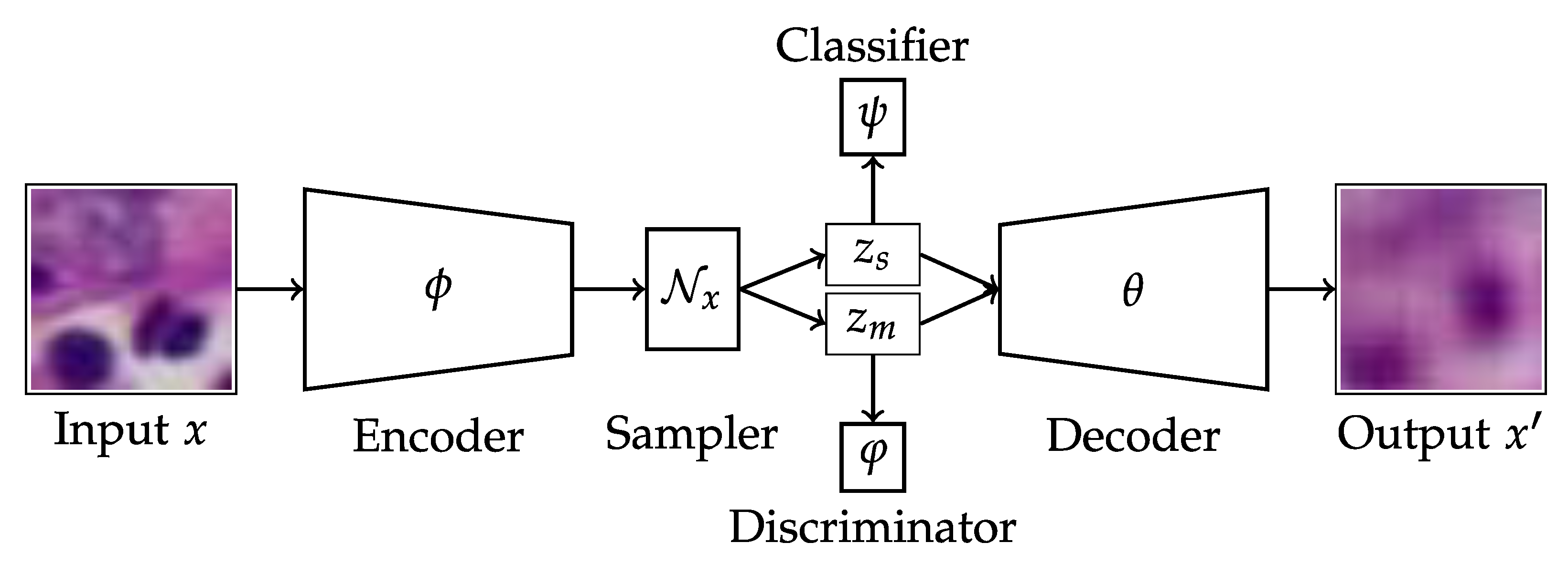
In general, an autoencoder consists in two main blocks (networks): an encoder and a decoder which are designed to perform (i) encoding of the input data into a lower dimensional latent embedding, and (ii) reconstruction of the input from the lower dimensional space. This can be seen as a composition of two functions such that the output where and are the encoder and decoder functions, respectively, and and are their corresponding parameters that are learned through an optimization process (Figure 1). The objective function for this optimization process could be, for example, the mean squared error or the cross entropy. The main goal when designing an autoencoder is to obtain a latent representation z of the input which captures the main traits of the modelled domain that generalise well to unseen data while being robust to noise. The encoded sample z can be obtained by drawing a sample from a multinormal distribution:
thereby yielding better generalization properties [20]. Several variants of the basic autoencoder have been proposed, including denoising autoencoder [21] and sparse autoencoder [22]. In the present work, the model is based on the variational autoencoder [23] for disentangled representation learning. The latent loss from the original variational autoencoder formulation by Kingma and Welling [20] is multiplied with a constant value . This additional weighting factor promotes independence of the latent dimensions as it enforces stronger similarity between the learned distribution and the standard multivariate normal prior. Independence between individual dimensions results in more disentangled features [24].
The basic components, namely the encoder, sampler, and decoder, are extended by a classifier and a discriminator, leveraging the class label information. In the context of differently stained histology images, the class label denotes the domain of the data (i.e., H&E or type of immune stain: CD44, FOXP3, etc.). The overall model architecture is depicted in Figure 1. Let be the set of categories in the data, with denoting the set cardinality, i.e., the number of different categories. The classifier is trained to predict the class label distribution
From activations approximating the true label from a subspace of the latent code for an input . Therefore, it serves as a measurement of class-related information contained in the code subset. The discriminator works in an equivalent way on the complementary subspace of the latent code, , predicting the same label. The difference lies in how the loss terms are used in updating the model parameters.
The weights of the individual network components, parameterized by and for the encoder, classifier, discriminator, and decoder respectively, are optimized with different objective functions during joint model training. The latent loss,
for a sample is computed as the Kullback-Leibler divergence between the encoder output (see Equation (2)) and the standard multivariate Gaussian prior with zero mean and diagonal covariance matrix with unit variances,
following [20] but with the additional weighting factor from [24] (see also Equation (8)). The reconstruction loss,
for an image (region) of width , height and number of channels , is based on the sum of absolute differences over the image domain. The supervised softmax classification loss functions are
and
respectively, and are minimized by updating the classifier and discriminator weights and . The joint encoder/decoder loss function combines the losses defined in Equations (3) and (5)–(7) into a single grand loss,
as a weighted sum of reconstruction loss ( latent loss classification loss , and discriminator loss . Note that the discriminator loss is used in an adversarial manner such that is optimized to maximize , but minimize . The respective terminology of an adversarial and a discriminator was initially introduced by Goodfellow in [25] and is by now heavily associated with generative adversarial networks (GANs). Despite not being a GAN-based approach, we decided to use the terms as the components have similar properties and purpose. The discriminator acts as a measurement of model performance, as low accuracy after training marks low content of stain-related information in , and the loss is used to update the weights of the encoder , similar to how the generative model is trained in a GAN approach.
By restricting the label-related information to a specific part of the latent code , the remaining part becomes domain-invariant as it contains structural information which is persistent across domains. A similar approach is also pursued in [26,27]. Disentangling the latent space allows further applications to decisively choose which features to include for the task at hand. This is already implicitly done by the classification network.
2.2.2. Network Architecture
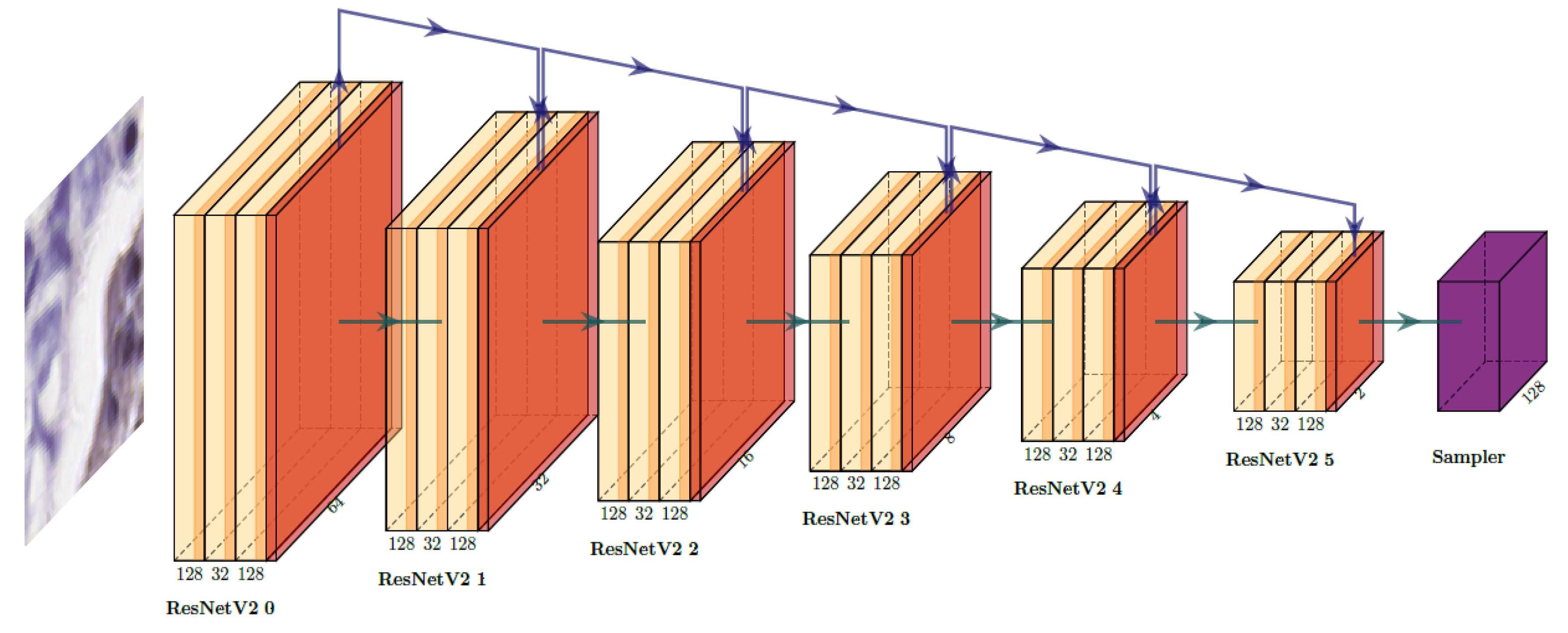
Residual layers with skip connections proposed by [28] are used for the encoder to provide stronger gradients and to increase the network depth in order to learn higher level features. Spatial down-sampling is achieved by maximum pooling layers while the ResNet blocks have a stride of 1 and use the implementation from [29]. The full encoder is shown in Figure 2.
The sampler activations are used as mean and lower triangle of the covariance matrix for having a multi-variate normal distribution, with , with prime indicating the matrix transposition. Then, for an input sample the encoder and sampler output are
The activation functions used are the identity mapping and the exponential function for the mean and covariance components, respectively.
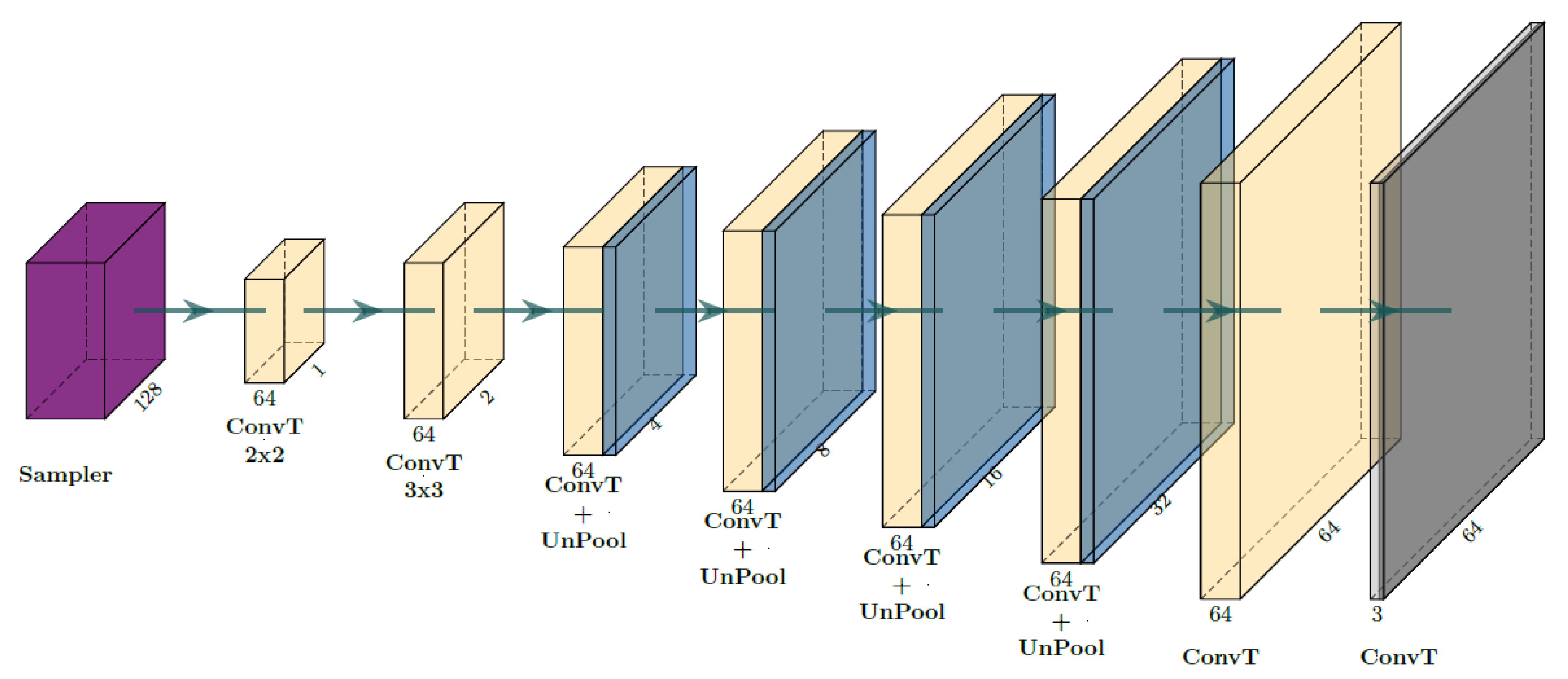
Following standard autoencoder conventions, the decoder approximately reconstructs the input by a series of deconvolution and up-sampling operations without residual skip connections. A kernel size of 2 is used for the first deconvolution to increase the spatial resolution like pooling layers, see Figure 3.
Both the classifier and the discriminator are single layer dense networks with weights, since the latent representation is already an abstract high-level representation of the raw data.
The final model used for the experiments was trained on 10,000,000 image patches of size 64 by 64 pixels for approximately 2,500,000 steps with a batch size of 256. The encoder is comprised of 6 ResNetV2 blocks with 2 units, followed by activation, batch normalization and pooling layers while the decoder has 8 transposed convolution, activation and batch norm layers, as well as 6 unpooling layers in order to restore the initial input shape.
2.2.3. Distances in the Latent Space
Once a model is trained, the latent representation of any input image can be obtained. Then, for any practical applications, a distance (or similarity function) needs to be defined which should satisfy the metric axioms and, hopefully, will capture the intended distance between the corresponding inputs . The stochastic process involved in obtaining z violates the first axiom, therefore we use a distance over the probability distributions.
Since the latent space representation of an input image is given by a multivariate Gaussian distribution, the distances between these representations cannot be computed as Euclidean distances. Let and be the two multivariate Gaussians corresponding to the latent vectors and . In our case, we tested two distances:
- Bhattacharyya distance (BD):
- Symmetrized Kullback–Leibler divergence (SKLD):where is Kullback–Leibler divergence as used in the latent loss from Equation (3). The Equation (11) further simplifies in the case of diagonal covariance matrices for the two distributions.
To measure the similarity of two patches, we therefore compute the Bhattacharyya distance given in Equation (10) or the symmetrized KL divergence from Equation (11) of the probability distributions defined by the encoder output for given input patches. We leverage the disentanglement properties of the model by choosing only the dimensions which capture the morphological information instead of the whole latent space, in order to measure the similarity in a stain independent manner. Therefore, only the probability space over the dimensions defining are used for the distance computation. Visualizations of the whole latent space and the subspaces using principal component analysis (PCA) and t-stochastic neighbour embedding (tSNE) are shown in Figure 4 and Figure 5 respectively.
2.2.4. Bag of Visual Words
The use of visual codebooks as basis for summarizing images has seen a lot of applications since it has been initially proposed [30], being successfully used in analysis of digital pathology images as well [31,32]. Generally, the method requires constructing a dictionary of visual words (a codebook) that will be used as templates for summarizing the images. An image is recoded in terms of this codebook by assigning to each local neighbourhood (usually small rectangular regions) a code representing the closest template from the codebook. After recoding, one can simply use the histograms of such codes as a summary of the image. For the construction of the codebook, the k-means clustering and the Gaussian Mixture Models (GMMs) are the most common choices [30], and are typically used with either standard bag-of-visual words or other aggregators. Jégou et al. [33] give a comprehensive comparison of various design choices.
For our case, the latent representation of the input images forbids the use of k-means of GMMs since these methods implicitly assume a Euclidean space for their input data. In our case, we resorted to use the symmetrized Kullback–Leibler divergence (Equation (11)) with DBSCAN clustering algorithm [34]. Since the algorithm does not identify centres of the clusters but rather core samples characterizing the clusters, we used the latter as the codewords in the dictionary.
2.2.5. Statistical Analyses
For comparing the results of patch matching in image registration scenario, we used Wilcoxon rank sum test for pairs of measurements (errors measures in pixels) with a predefined significance level When analysing the results of image summarization for intra-tumour heterogeneity scenario, we used hierarchical clustering with Ward distance for clustering histograms of codewords (with Earth-mover distance between histograms). All statistical analyses were performed in R version 3.6.2.
3. Results
We have implemented the method described above in Python, using Tensorflow 1.12 library. The code and a number of trained models are available from https://github.com/hechth/dpath_gae.
3.1. Latent Space Disentanglement
The disentanglement properties of the trained model were assessed visually by inspecting latent graphical representations of the learnt latent space, such as PCA and tSNE. The embedding of the whole latent space using tSNE (Figure 4) shows clear clustering of the data according to morphology and staining.
The subspaces and were visualized using PCA (Figure 5) and label related colouring to emphasize on the distribution of identically stained images. The subspace used for stain prediction by the classifier has a tight label related coupling while the structural embedding in the complementary part indicates loose stain related clustering, but morphologically similar image patches are grouped together.
3.2. Image Registration Scenario
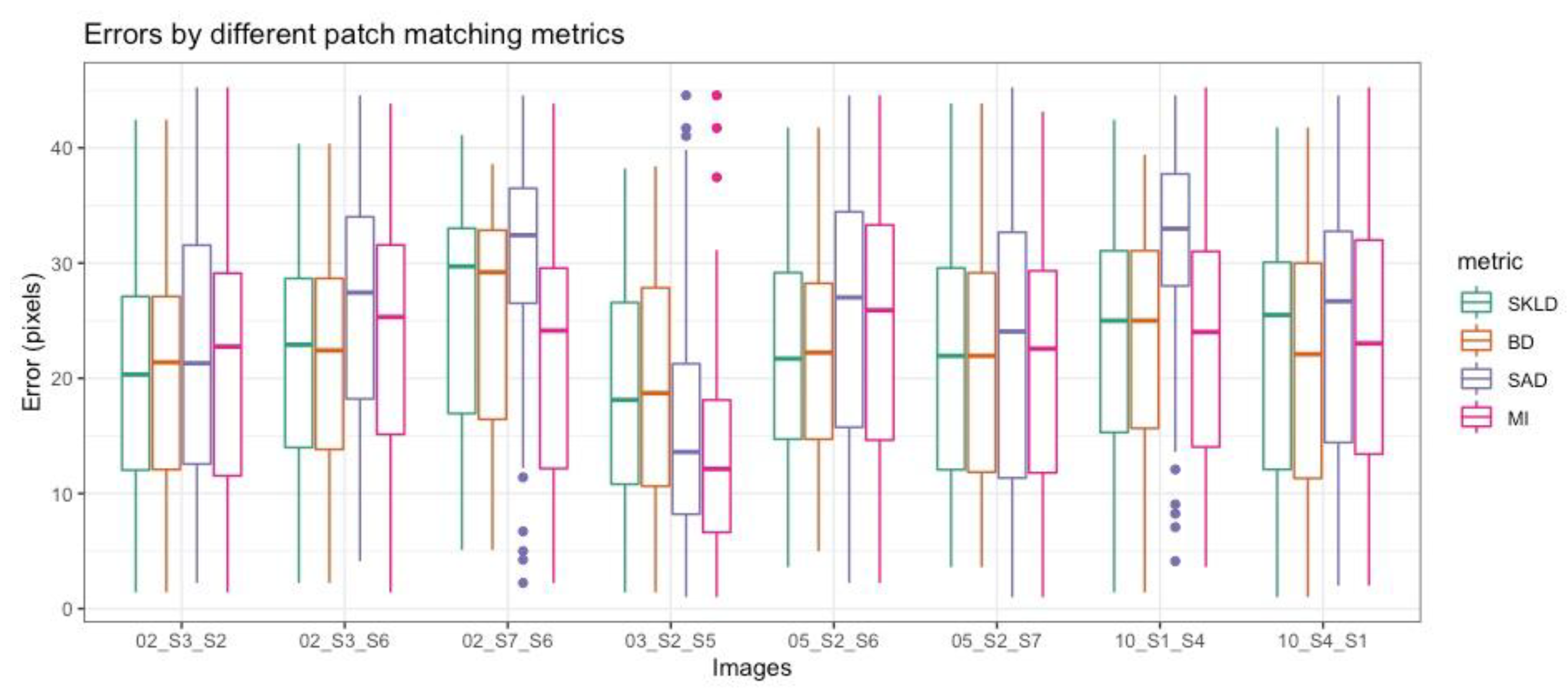
We compared the performance of our method with patch-based adaptations of (i) sum of absolute differences and (ii) mutual information. For a given set of corresponding landmarks in two images, we computed the similarity of patches extracted at the landmark positions in the source image with all positions in a 64 × 64 window around the corresponding landmark in the target image. The score was calculated as the distance between the position with the best similarity value and the actual landmark position in the target image. This score was averaged over all landmarks for eight different image pairs coming from the ANHIR 2019 challenge dataset. Each image pair had between 60 and 90 landmarks, 676 in total
In Figure 6 boxplots of differences between the best matching position and the hand-marked landmarked are shown for each of the considered metrics. Summaries of these distances are given in Table 1. Only in two cases were the differences between any of the new metric and the mutual information statistically significant (p < 0.05 for Wilcoxon rank sum test): in one case (03_S2_S5), MI was superior to the two proposed distances, while in the second case (05_S2_S6), MI was inferior. Thus, the two new distances seem to perform similarly to MI, while outperforming the raw pixel-based metric (SAD). At the same time, the stability of the new metric seems to be slightly better than the other two, as shown by the lower standard deviation of the corresponding errors (Table 1).
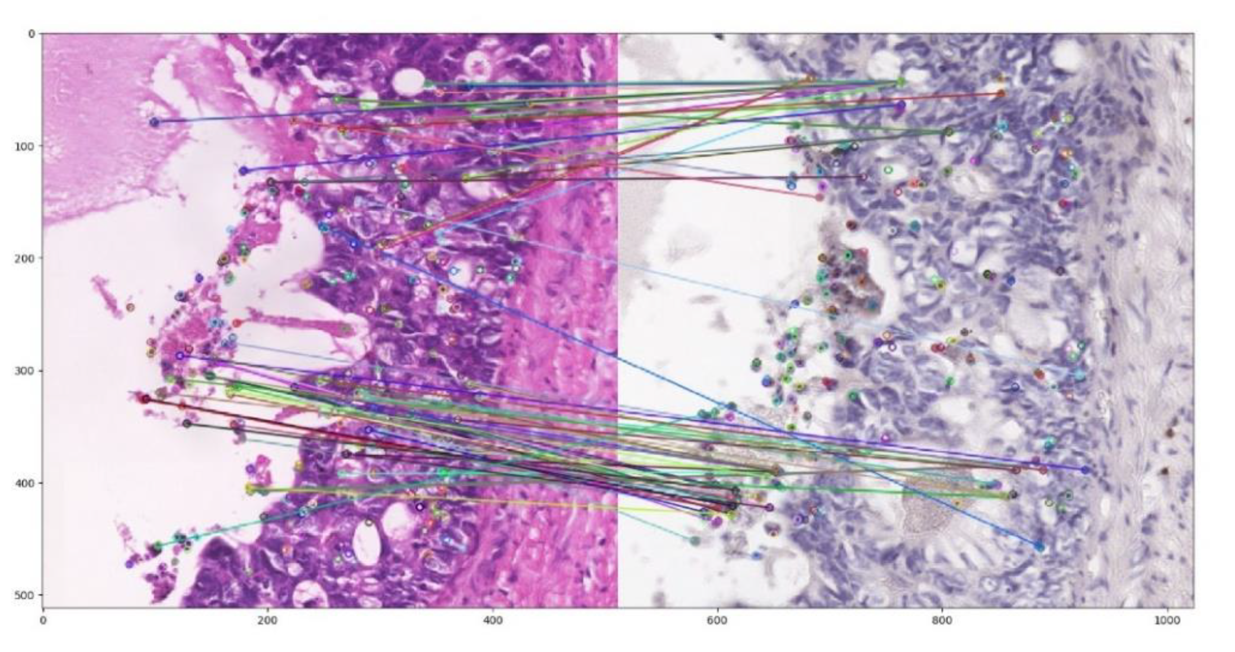
We also explored the applicability of the novel feature extraction method and similarity metric for two different image registration algorithms. We developed a deformable image registration method based on ITK, akin to the methods presented in [35]. The second approach matches ORB key-points extracted using OpenCV using our similarity metric. Neither of the approaches yielded viable results, as can be seen in Figure 7. Both methods are open for further development.
3.3. Intra-Tumour Heterogeneity Scenario
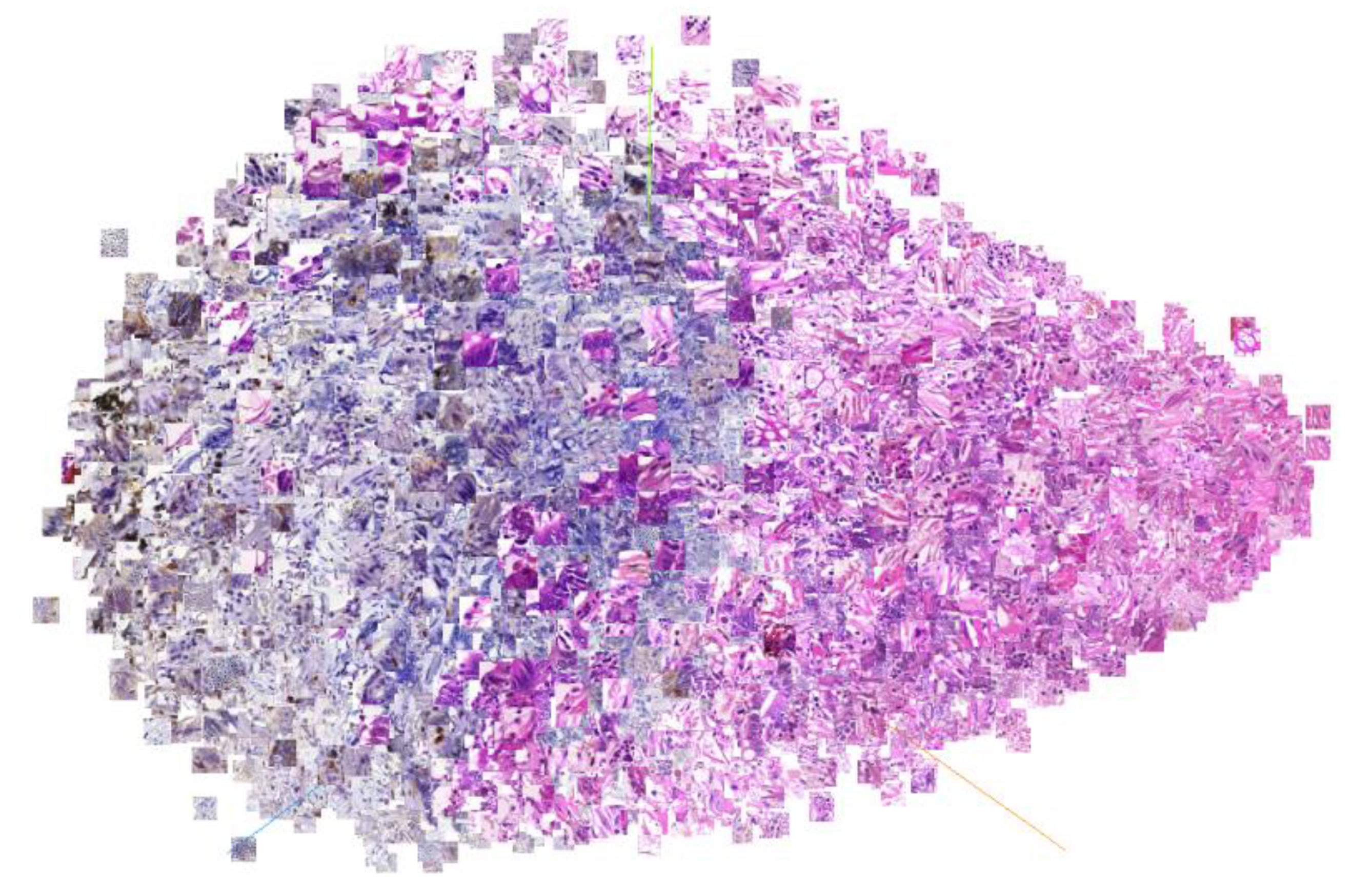
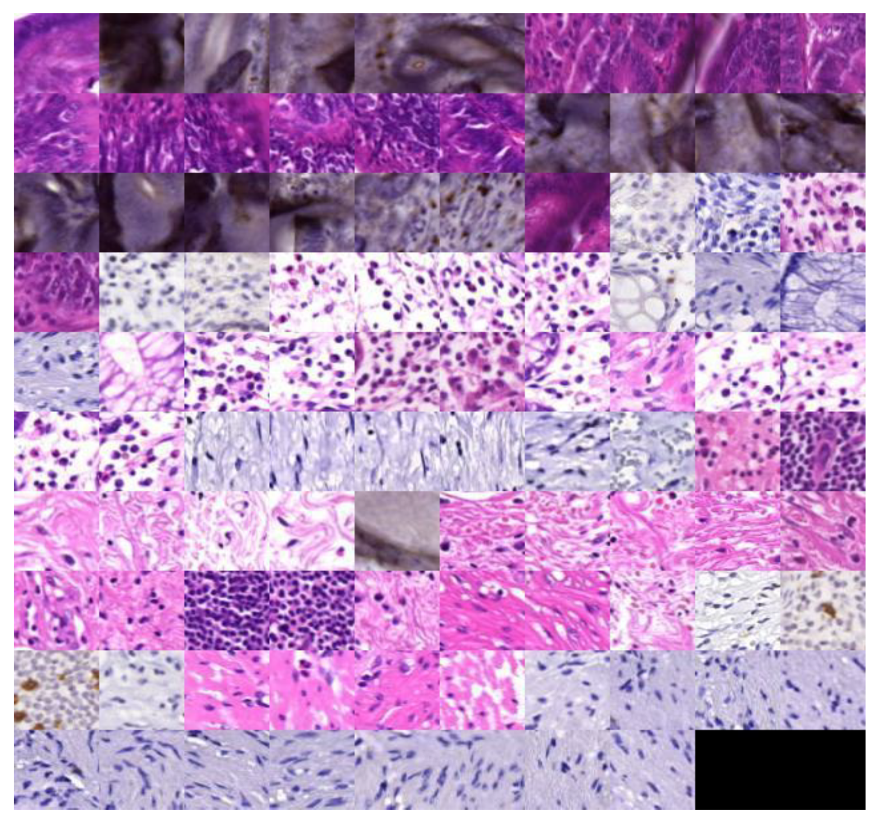
For the second set of experiments, we constructed a visual codebook using the latent representation of patches. Since we were interested in regions with higher content (in terms of cells), we excluded (before building the codebook) all the close-to-constant image patches (standard deviation of the average over channels below 0.25). The resulting codebook had codewords and the image patches corresponding to the codewords in the latent space are shown in Figure 8. It is immediately apparent that the selected codewords originate from slides with different types of staining and some can be easily labelled as representing epithelial cells, immune cells, or mucosa regions.
For each image (30 images, three different stains in 10 series), we computed their representation based on the visual codebook and summarized it in terms of histograms which could be seen as a descriptor of the heterogeneity (of the tissue).
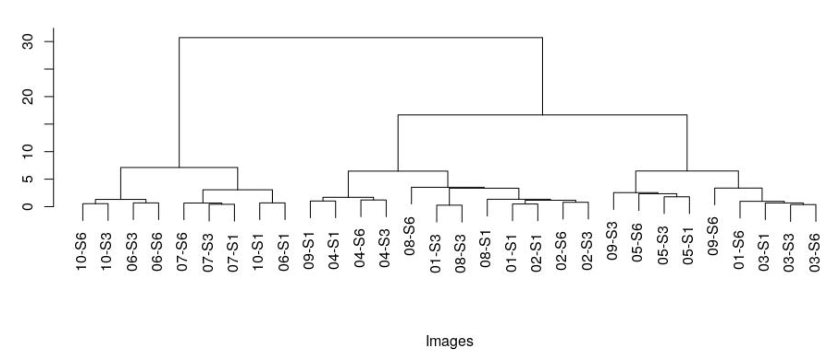
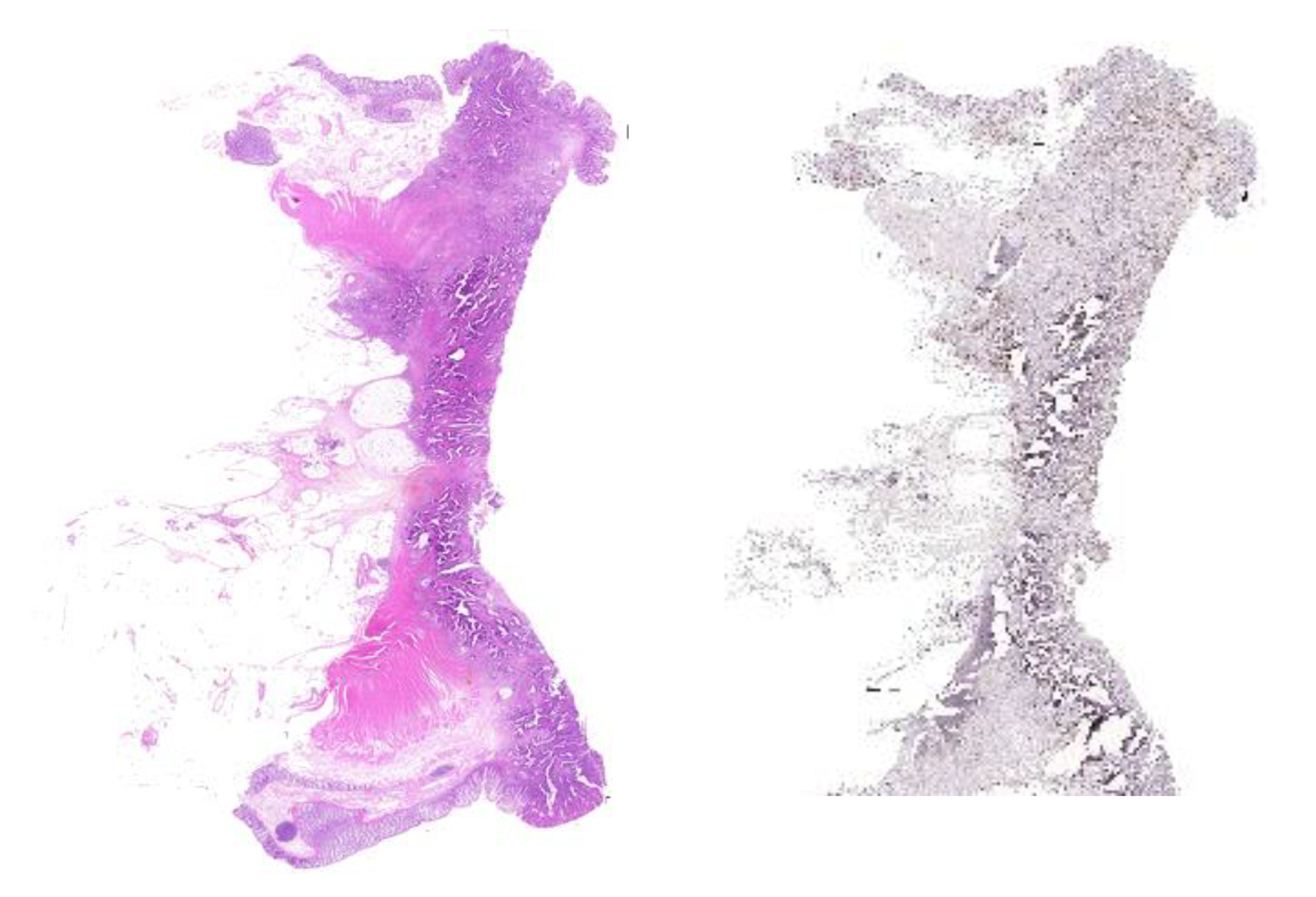
We wanted to assess the efficiency of this simple summaries to capture the image content, thus we clustered the corresponding histograms. The resulting dendrogram is shown in Figure 9. The results are mixed: for some series (e.g., 03, 04, 05, or 07) the three stains cluster closely, while for others (e.g., 01) the different stains are further apart. By inspecting these cases, we have noticed that the tissue was torn and section truncated, clearly impacting negatively on the matching between the slides (Figure 10).
4. Discussion
Having features that capture the textural/morphological aspects independent of the staining would allow learning models across different immune stainings. Such models can be applied to image registration or image retrieval problems as well as to more explorative scenarios such as characterization of tissue heterogeneity. In the proof-of-concept applications we presented here we used pathology sections from colon cancer cases. However, the method is by no means bound to any specific pathology.
We trained an autoencoder to produce a disentangled representation in the latent space with the purpose of separating the colour/stain information from the structure information. The obtained representation was tested in scenarios inspired by real-world applications: cross-stain registration of images and comparison of intra-tumour heterogeneity. We stress the fact that these are proof-of-concept analyses with the purpose of studying the possibility of achieving stain invariant feature extraction.
In the first scenario, the results indicate that the newly proposed approach is able to extract relevant information for comparing patches across stains with similar performance as the mutual information distance. The novel method has several advantages over mutual information. The use of probability-based similarity measures (SKLD, BD) makes the approach invariant to identical perturbations of the compared datasets. Further, the model uses data driven features for similarity estimation, explicitly separating feature selection and similarity estimation. Finally, the inference step is computationally efficient.
In the second scenario, we used the same latent representation as before for learning a visual codebook. Since the latent representation is parametrized as a multivariate Gaussian distribution, there is a need for careful selection of the metric to be used in clustering such representations. In our case, we used the SKLD with diagonal Gaussians and a clustering algorithm able to accommodate non-Euclidean distances (DBSCAN). The resulting codebook was used for summarizing the images in terms of histograms (of codewords), as simple descriptors of intra-tumoral heterogeneity. Then, using hierarchical clustering, we showed that most of the series (consecutive sections from the same block) cluster together. There were also some cases which appeared to be distant in the hierarchical clustering. Technical issues, such as tissue tearing and fragmentation, are definitely contributing to these results (Figure 10). A further application of this approach, not detailed here, is semantic image retrieval: retrieving slide images with similar tissue morphology mix, across different immune stains. At the core, this would application could have an image summarization based on multi-stain visual dictionaries, an extended version of the one developed here.
The latent representation was learned from a set of images in an application-agnostic manner, with no tuning for the latter usage. In a more realistic case, the representation and the latter distance (or visual codebook) would need to be adapted and optimized. Comparing pathology sections across stains is feasible with the approach described above, however better summarization would be needed for capturing the tissue heterogeneity. The results presented here were obtained on a rather limited data set. Clearly, scaling up both the training set and the test set(s) is needed for achieving high confidence in the novel representation.
5. Conclusions
We proposed a disentangled autoencoder for learning cross-staining representation of whole slide images. The learnt latent representation was used in two realistic applications and its performance deemed satisfactory and promising for a basic model. There are a number of alternative usages for the presented approach that were not discussed here, e.g., virtual staining of the slides (one would alter the latent representation in the subspace corresponding to the stain) or stain normalization (with structure separated from stain, a standard stain reconstruction could be obtained). It is also clear that, for optimal performance, the architecture (and the models provided) need further fine tuning to the intended application.
Supplementary Materials
The following are available online at https://www.mdpi.com/2076-3417/10/18/6427/s1, Table S1: The list of samples from ANHIR collection used in the reported experiments.
Author Contributions
Conceptualization, H.H. and V.P.; methodology, H.H., M.H.S., and V.P.; software, H.H.; validation, H.H. and M.H.S.; writing—original draft preparation, H.H., M.H.S., and V.P.; visualization, H.H.; supervision, V.P.; funding acquisition, V.P. All authors have read and agreed to the published version of the manuscript.
Funding
This project was funded by the Grantová Agentura České Republiky (GAČR-Czech Science Foundation) through grant number GA17-15361S.
Acknowledgments
We acknowledge the support of the RECETOX research infrastructure through the grant LM2018121 of the Czech Ministry of Education, Youth and Sports as well as of the CETOCOEN EXCELLENCE Teaming 2 project supported by Horizon2020 (857560) and the Czech ministry of Education, Youth and Sports (02.1.01/0.0/0.0/18_046/0015975).
Conflicts of Interest
The authors declare no conflict of interest. The funders had no role in the design of the study; in the collection, analyses, or interpretation of data; in the writing of the manuscript, or in the decision to publish the results.
References
- Madabhushi, A.; Lee, G. Image analysis and machine learning in digital pathology: Challenges and opportunities. Med. Image Anal. 2016, 33, 170–175. [Google Scholar] [CrossRef] [PubMed] [Green Version]
- Niazi, M.K.K.; Parwani, A.V.; Gurcan, M.N. Digital pathology and artificial intelligence. Lancet Oncol. 2019, 20, e253–e261. [Google Scholar] [CrossRef]
- Viergever, M.A.; Maintz, J.B.A.; Klein, S.; Murphy, K.; Staring, M.; Pluim, J.P.W. A survey of medical image registration—Under review. Med. Image Anal. 2016, 33, 140–144. [Google Scholar] [CrossRef] [PubMed] [Green Version]
- Ruifrok, A.C.; Johnston, D.A. Quantification of histochemical staining by color deconvolution. Anal. Quant. Cytol. Histol. 2001, 23, 291–299. [Google Scholar] [PubMed]
- van der Loos, C.M. Multiple Immunoenzyme Staining: Methods and Visualizations for the Observation With Spectral Imaging. J. Histochem. Cytochem. 2008, 56, 313–328. [Google Scholar] [CrossRef] [PubMed] [Green Version]
- Alsubaie, N.; Trahearn, N.; Raza, S.E.A.; Snead, D.; Rajpoot, N.M. Stain Deconvolution Using Statistical Analysis of Multi-Resolution Stain Colour Representation. PLoS ONE 2017, 12, e0169875. [Google Scholar] [CrossRef] [PubMed]
- Macenko, M.; Niethammer, M.; Marron, J.S.; Borland, D.; Woosley, J.T.; Guan, X.; Schmitt, C.; Thomas, N.E. A method for normalizing histology slides for quantitative analysis. In Proceedings of the Proceedings—2009 IEEE International Symposium on Biomedical Imaging: From Nano to Macro, Boston, MA, USA, 28 June–1 July 2009; pp. 1107–1110. [Google Scholar]
- Gurcan, M.N.; Boucheron, L.E.; Can, A.; Madabhushi, A.; Rajpoot, N.M.; Yener, B. Histopathological image analysis: A review. IEEE Rev. Biomed. Eng. 2009, 2, 147–171. [Google Scholar] [CrossRef] [PubMed] [Green Version]
- Kather, J.N.; Weis, C.-A.; Bianconi, F.; Melchers, S.M.; Schad, L.R.; Gaiser, T.; Marx, A.; Zöllner, F.G. Multi-class texture analysis in colorectal cancer histology. Sci. Rep. 2016, 6, 27988. [Google Scholar] [CrossRef] [PubMed]
- Wang, D.; Khosla, A.; Gargeya, R.; Irshad, H.; Beck, A.H. Deep Learning for Identifying Metastatic Breast Cancer. arXiv 2016, arXiv:1606.05718. [Google Scholar]
- Kather, J.N.; Krisam, J.; Charoentong, P.; Luedde, T.; Herpel, E.; Weis, C.-A.; Gaiser, T.; Marx, A.; Valous, N.A.; Ferber, D.; et al. Predicting survival from colorectal cancer histology slides using deep learning: A retrospective multicenter study. PLoS Med. 2019, 16, e1002730. [Google Scholar] [CrossRef]
- Rumelhart, D.E.; Hinton, G.E.; Williams, R.J. Learning internal representations by error propagation. In Parallel Distributed Processing: Explorations in the Microstructure of Cognition: Foundations; MIT Press: Cambridge, MA, USA, 1987; pp. 318–362. [Google Scholar]
- Hinton, G.E.; Osindero, S.; Teh, Y.W. A fast learning algorithm for deep belief nets. Neural Comput. 2006, 18, 1527–1554. [Google Scholar] [CrossRef]
- Bengio, Y.; LeCun, Y. Scaling Learning Algorithms toward AI. In Large-Scale Kernel Machines; Bottou, L., Chapelle, O., DeCoste, D., Weston, J., Eds.; MIT Press: Cambridge, MA, USA, 2007. [Google Scholar]
- Erhan, D.; Courville, A.; Bengio, Y.; Vincent, P. Why does unsupervised pre-training help deep learning? J. Mach. Learn. Res. 2010, 9, 201–208. [Google Scholar]
- Xu, J.; Xiang, L.; Liu, Q.; Gilmore, H.; Wu, J.; Tang, J.; Madabhushi, A. Stacked sparse autoencoder (SSAE) for nuclei detection on breast cancer histopathology images. IEEE Trans. Med Imaging 2016, 35, 119–130. [Google Scholar] [CrossRef] [PubMed] [Green Version]
- Hou, L.; Nguyen, V.; Kanevsky, A.B.; Samaras, D.; Kurc, T.M.; Zhao, T.; Gupta, R.R.; Gao, Y.; Chen, W.; Foran, D.; et al. Sparse autoencoder for unsupervised nucleus detection and representation in histopathology images. Pattern Recognit. 2019, 86, 188–200. [Google Scholar] [CrossRef] [PubMed]
- Janowczyk, A.; Basavanhally, A.; Madabhushi, A. Stain Normalization using Sparse AutoEncoders (StaNoSA): Application to digital pathology. Comput. Med Imaging Graph. 2017, 57, 50–61. [Google Scholar] [CrossRef] [PubMed] [Green Version]
- Awan, R.; Rajpoot, N. Deep Autoencoder Features for Registration of Histology Images. In Proceedings of the Medical Image Understanding and Analysis, Houston, TX, USA, 10 February 2018; Springer: Cham, Switzerland, 2018; pp. 371–378. [Google Scholar]
- Kingma, D.P.; Welling, M. Auto-Encoding Variational Bayes. In Proceedings of the International Conference on Learning Representations, Banff, AB, Canada, 14–16 April 2014. [Google Scholar]
- Vincent, P.; Larochelle, H.; Bengio, Y.; Manzagol, P.-A. Extracting and composing robust features with denoising autoencoders. In Proceedings of the 25th International Conference on Machine Learning, Helsinki, Finland, 5–9 July 2008. [Google Scholar]
- Coates, A.; Ng, A.Y. Learning Feature Representations with K-Means. In Neural Networks: Tricks of the Trade, 2nd ed.; Springer: Berlin, Germany, 2012; Volume 7700, pp. 561–580. [Google Scholar]
- Higgins, I.; Matthey, L.; Pal, A.; Burgess, C.; Glorot, X.; Botvinick, M.; Mohamed, S.; Lerchner, A. Β-VAE: Learning basic visual concepts with a constrained variational framework. In Proceedings of the 5th International Conference on Learning Representations, ICLR 2017—Conference Track Proceedings, Toulon, France, 24–26 April 2017. [Google Scholar]
- Burgess, C.P.; Higgins, I.; Pal, A.; Matthey, L.; Watters, N.; Desjardins, G.; Lerchner, A. Understanding disentangling in β-VAE. In Proceedings of the 2017 NIPS Workshop on Learning Disentangled Representations, Long Beach, CA, USA, 4–9 December 2017. [Google Scholar]
- Goodfellow, I.J.; Pouget-Abadie, J.; Mirza, M.; Xu, B.; Warde-Farley, D.; Ozair, S.; Courville, A.; Bengio, Y. Generative adversarial nets. In Proceedings of the 27th International Conference on Neural Information Processing Systems—Volume 2, Montreal, QC, Canada, 8–13 December 2014; MIT Press: Cambridge, MA, USA, 2014; pp. 2672–2680. [Google Scholar]
- Tzeng, E.; Hoffman, J.; Saenko, K.; Darrell, T. Adversarial Discriminative Domain Adaptation. Comput. Res. Repos. (CoRR) 2017, abs/1702.0, 7167–7176. [Google Scholar]
- Qin, C.; Shi, B.; Liao, R.; Mansi, T.; Rueckert, D.; Kamen, A. Unsupervised Deformable Registration for Multi-Modal Images via Disentangled Representations. Comput. Res. Repos. (CoRR) 2019, abs/1903.0, 249–261. [Google Scholar]
- He, K.; Zhang, X.; Ren, S.; Sun, J. Deep Residual Learning for Image Recognition. In Proceedings of the 2016 IEEE Conference on Computer Vision and Pattern Recognit. (CVPR), Los Angeles, CA, USA, 26 June–1 July 2016; IEEE: New York, NY, USA, 2016; pp. 770–778. [Google Scholar]
- He, K.; Zhang, X.; Ren, S.; Sun, J. Identity Mappings in Deep Residual Networks. Lecture Notes in Computer Science. In Proceedings of the ECCV 2016, Amsterdam, The Netherlands, 11–14 October 2016. [Google Scholar]
- Csurka, G.; Dance, C.; Fan, L. Visual categorization with bags of keypoints. In Proceedings of the ECCV International Workshop on Statistical Learning in Computer Vision 2004, Prague, Czech Republic, 11–14 May 2004; Springer: Cham, Switzerland, 2004. [Google Scholar]
- Caicedo, J.C.; Cruz, A.; Gonzalez, F.A. Histopathology Image Classification Using Bag of Features and Kernel Functions. In Proceedings of the 12th Conference on Artificial Intelligence in Medicine, Verona, Italy, 18–22 July 2009; Combi, C., Shahar, Y., Abu-Hanna, A., Eds.; Springer: Berlin/Heidelberg, Germany; Verona, Italy, 2009; pp. 126–135. [Google Scholar]
- López-Monroy, A.P.; Montes-y-Gómez, M.; Escalante, H.J.; Cruz-Roa, A.; González, F.A. Bag-of-Visual-Ngrams for Histopathology Image Classification. In Proc SPIE 8922, IX International Seminar on Medical Information Processing and Analysis; Mexico City, Mexico, 11–14 November 2013; Brieva, J., Escalante-Ramírez, B., Eds.; SPIE: Bellingham, WA, USA, 2013. [Google Scholar]
- Jégou, H.; Perronnin, F.; Douze, M.; Sanchez, J.; Perez, P.; Schmid, C. Aggregating Local Image Descriptors into Compact Codes. IEEE Trans. Pattern Anal. Mach. Intell. 2012, 34, 1704–1716. [Google Scholar] [CrossRef] [PubMed] [Green Version]
- Ester, M.; Kriegel, H.-P.; Sander, J.; Xu, X. A density-based algorithm for discovering clusters a density-based algorithm for discovering clusters in large spatial databases with noise. In Proceedings of the KDD’96: Proceedings of the Second International Conference on Knowledge Discovery and Data Mining, Portland, OR, USA, 2–4 August 1996; pp. 226–231. [Google Scholar]
- Simonovsky, M.; Gutiérrez-Becker, B.; Mateus, D.; Navab, N.; Komodakis, N. A Deep Metric for Multimodal Registration. arXiv 2016, arXiv:1609.05396. [Google Scholar]
Figure 1.
Architecture for the proposed model, extending the β-Variational Autoencoder with a supervised classifier and discriminator component.
Figure 1.
Architecture for the proposed model, extending the β-Variational Autoencoder with a supervised classifier and discriminator component.

Figure 2.
Architecture of the encoder part, comprising of ResNet v2 blocks with skip connections and information bottleneck layers.
Figure 2.
Architecture of the encoder part, comprising of ResNet v2 blocks with skip connections and information bottleneck layers.

Figure 3.
Layout of the decoder without skip connections to reconstruct the input.

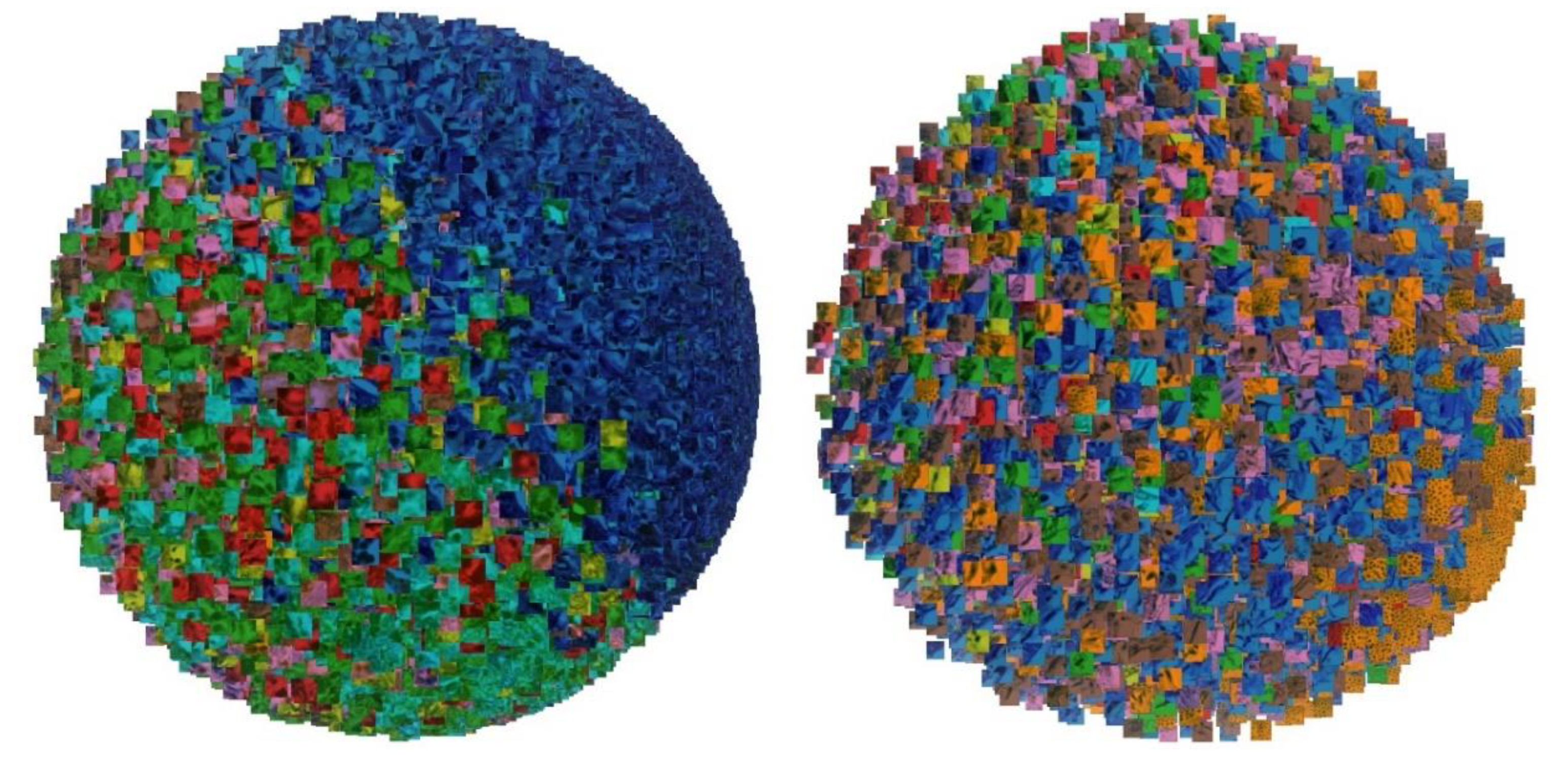
Figure 4.
tSNE plot of the learnt latent space, indicating stain and structure related grouping.

Figure 5.
PCA of the stain (left) and morphology (right) subspaces. Coloring indicates the label (staining) and the data was subjected to a sphering (whitening) transformation for better visualization.
Figure 5.
PCA of the stain (left) and morphology (right) subspaces. Coloring indicates the label (staining) and the data was subjected to a sphering (whitening) transformation for better visualization.

Figure 6.
Comparison of four distances for patch-matching. Eight different stains pairs (denoted Si_Sj) were tested with four difference metrics: symmetrized Kullback-Leibler divergence (SKLD), Bhattacharyya distance (BD), sum of absolute deviations (SAD) and mutual information (MI), respectively. Only two cases showed statistically significant differences: 03_S2_S5 and 05_S2_S6.

Figure 7.
Key-point matching using the learnt model and OpenCV based ORB extractor. 64 × 64 sized patches are extracted at the key-points and matched according to the minimal Bhattacharyya distance. The best 100 matches out of 500 points per image are shown as connected pair.
Figure 7.
Key-point matching using the learnt model and OpenCV based ORB extractor. 64 × 64 sized patches are extracted at the key-points and matched according to the minimal Bhattacharyya distance. The best 100 matches out of 500 points per image are shown as connected pair.

Figure 8.
Image patches corresponding to the core components selected by DBSCAN in latent space and defining the codewords of the learned visual codebook.
Figure 8.
Image patches corresponding to the core components selected by DBSCAN in latent space and defining the codewords of the learned visual codebook.

Figure 9.
Hierarchical clustering of histograms of codewords. “Si” indicates a stain.

Figure 10.
Example of sections with poorly matching histograms of codewords.


Table 1.
Average, standard deviation and median error in pixels for all data for the compared similarity metrics.
Table 1.
Average, standard deviation and median error in pixels for all data for the compared similarity metrics.
| Error (Pixels) | SKLD | BD | SAD | MI |
|---|---|---|---|---|
| Average (Std. dev) | 21.8 (10.2) | 21.7 (10.2) | 24.8 (12.0) | 21.6 (11.1) |
| Median | 22.3 | 22.1 | 26.7 | 22.7 |
© 2020 by the authors. Licensee MDPI, Basel, Switzerland. This article is an open access article distributed under the terms and conditions of the Creative Commons Attribution (CC BY) license (http://creativecommons.org/licenses/by/4.0/).
Share and Cite
MDPI and ACS Style
Hecht, H.; Sarhan, M.H.; Popovici, V. Disentangled Autoencoder for Cross-Stain Feature Extraction in Pathology Image Analysis. Appl. Sci. 2020, 10, 6427. https://doi.org/10.3390/app10186427
AMA Style
Hecht H, Sarhan MH, Popovici V. Disentangled Autoencoder for Cross-Stain Feature Extraction in Pathology Image Analysis. Applied Sciences. 2020; 10(18):6427. https://doi.org/10.3390/app10186427
Chicago/Turabian StyleHecht, Helge, Mhd Hasan Sarhan, and Vlad Popovici. 2020. "Disentangled Autoencoder for Cross-Stain Feature Extraction in Pathology Image Analysis" Applied Sciences 10, no. 18: 6427. https://doi.org/10.3390/app10186427
Note that from the first issue of 2016, this journal uses article numbers instead of page numbers. See further details here.