Surrogate Models for Estimating Failure in Brittle and Quasi-Brittle Materials

Abstract

In brittle fracture applications, failure paths, regions where the failure occurs and damage statistics, are some of the key quantities of interest (QoI). High-fidelity models for brittle failure that accurately predict these QoI exist but are highly computationally intensive, making them infeasible to incorporate in upscaling and uncertainty quantification frameworks. The goal of this paper is to provide a fast heuristic to reasonably estimate quantities such as failure path and damage in the process of brittle failure. Towards this goal, we first present a method to predict failure paths under tensile loading conditions and low-strain rates. The method uses a k-nearest neighbors algorithm built on fracture process zone theory, and identifies the set of all possible pre-existing cracks that are likely to join early to form a large crack. The method then identifies zone of failure and failure paths using weighted graphs algorithms. We compare these failure paths to those computed with a high-fidelity fracture mechanics model called the Hybrid Optimization Software Simulation Suite (HOSS). A probabilistic evolution model for average damage in a system is also developed that is trained using 150 HOSS simulations and tested on 40 simulations. A non-parametric approach based on confidence intervals is used to determine the damage evolution over time along the dominant failure path. For upscaling, damage is the key QoI needed as an input by the continuum models. This needs to be informed accurately by the surrogate models for calculating effective moduli at continuum-scale. We show that for the proposed average damage evolution model, the prediction accuracy on the test data is more than 90%. In terms of the computational time, the proposed models are $\approx \mathcal{O}\left({10}^6\right)$ times faster compared to high-fidelity fracture simulations by HOSS. These aspects make the proposed surrogate model attractive for upscaling damage from micro-scale models to continuum models. We would like to emphasize that the surrogate models are not a replacement of physical understanding of fracture propagation. The proposed method in this paper is limited to tensile loading conditions at low-strain rates. This loading condition corresponds to a dominant fracture perpendicular to tensile direction. The proposed method is not applicable for in-plane shear, out-of-plane shear, and higher strain rate loading conditions.

1. Introduction

Brittle fracture is a complex phenomena determined by interaction among several microstructural features of the material under study. These features include grain size, presence of pre-existing cracks or defects and/or pores, frictional characteristics, etc. [1,2]. When a brittle material containing pre-existing cracks is loaded, stresses concentrate around the crack tips [3,4]. When these cracks propagate they interact with other defects and cracks in their neighborhood. This results in a complex state of stress near the crack tips. Especially at lower strain rates, pre-existing cracks act as nucleation points for the generation of new cracks [5,6]. Nucleation, growth, and coalescence of pre-existing cracks results in the degradation of elastic properties in brittle materials, eventually causing catastrophic failure. This is because the critical amount of damage before rapid and unassisted crack growth can be limited in brittle materials. Moreover, damage accumulation also results in non-linear material behavior, a further challenge for the development of predictive models. Due to the prevalence of brittle materials in several applications in geosciences (e.g., hydraulic fracturing, geothermal, etc.) [7,8,9], infrastructure [5] and aerospace industry [10], fast and accurate models of brittle fracturing are needed.

Many constitutive models and numerical methods (e.g., seminal works of James Rice, John Hutchinson, Alan Needleman, Ravi-Chandar, Wolfgang Knauss, Zhigang Suo, Huajian Gao, Ares Rosakis, Emmanuel Detournay, etc.) have been proposed in the literature [11,12,13,14,15,16,17,18,19,20] that simulate processes such as crack initiation, crack propagation, and crack shielding in brittle materials. Foundational work by Griffith [21] and Irwin [22] explained how crack growth can be understood as a free energy balance between the surface energy generated by crack formation and the elastic energy released by the crack as it grows, and the crack tip stress intensity factors. However, Griffith’s theory over-predicts the fracture toughness as it does not consider the presence of other defects. Shortly thereafter, Barenblatt [23] and Dugdale [24] proposed the idea of a cohesive zone or fracture process zone (FPZ) preceding a crack tip. These ideas have been extensively expanded on in the past decades (e.g., works by Needleman, Beltz, Rice, Freed, Banks-Sills, Paulino, Roesler, Ortiz, Pandolfi, etc.) [25,26,27,28,29,30].

The current computing power available has allowed for complex fracture models to be applied to a wide range of length scales [31,32]. Of these, many continuum (or macro-scale) and phase-field modeling approaches [33,34,35,36,37,38,39] have been developed to address crack evolution and the overall material response in large samples (cm-scale and larger) including finite element methods [40,41,42] and boundary element methods [43,44]. Continuum-based approaches [45] assume that the computational domain can be treated as one continuous body. However, the nature of brittle fracture, which often results from growth and coalescence of major flaws, can be extremely localized and therefore not amenable to standard homogenization approaches. This often results in the emergence of a non-physical length scale within the numerical methods used to implement continuum models that can significantly impact the calculated material response [46]. Hence, these numerical methods cannot account for localized strains without further enhancement of the mathematical formulation [46,47]. Discrete element methods [32,48] are another class of modeling techniques available at the same length scale as continuum approaches. With these approaches, material is modeled as a collection of discrete blocks or particles that can displace and rotate with respect to each other, and even completely separate or break apart. Similarly, there are combined finite-discrete element methods (FDEM) that also have discrete material blocks, which can deform themselves due to further resolution of each block with finite elements [42,49,50,51,52,53]. In the FDEM methods, the discontinuities of interest (e.g., micro-cracks) must be on similar scale to the computational domain. Of all these approaches available in the fracture mechanics literature, we adopt the FDEM approach in this work. FDEM merges many features of other methods listed above. The high-fidelity FDEM model used in this work that accounts for fracture propagation was developed in a multi-physics software tool called Hybrid Optimization Software Suite (HOSS) [54,55].

Although, FDEM models have been shown to accurately model brittle fracture, the use of these models (e.g., HOSS) in realistic simulations is computationally intractable as they resolve all the individual cracks with highly resolved meshes and small time-steps at large-scales. Despite the increased realism in the physics and parallel implementation, we are still unable to capture the full range of spatial or temporal scales due to the large computational requirements of our applications, such as hydraulic fracturing [7] or underground nuclear explosion monitoring [56]. Coarsening of the domain and simplification of the physics [57,58] are commonly used workarounds, but these methods eliminate critical topological features (critical effects of crack-to-crack interactions) and as a result, predictions routinely fail to match observations [59,60]. One then has to resort to upscaling methods where the domain is split into several grid cells and the material properties in each grid cell are obtained from QoI such as failure paths and damage statistics, which are still computationally challenging. For example, to obtain the results for each HOSS simulation presented in this work, 4 hours of computation time on 400 processors were necessary. In addition, the amount of data being generated is also quite significant. That is, each simulation took up to 11.5 GB of disk space to store all the information needed to characterize different fracture propagation stages. Even for a very coarse upscaled domain of say 1000 cells, this leads to 1.6 M CPU-hours and 11.5 TB of disk space. For this reason, we need an approach that can provide key quantities of interest (QoIs) in a matter of seconds and with reasonable accuracy. This is the aim of the present work. We develop surrogate models for estimating the damage statistics along failure paths to inform continuum models. These surrogate models are built using data from HOSS high-fidelity numerical simulations. The proposed methods presented in this work are applicable only under low-strain rates and Mode I failure or tensile loading conditions. In these conditions, a single dominant fracture perpendicular to tensile loading is observed. A limitation of the proposed methodology is that it is not applicable for other modes of fracture and high strain rates loading conditions but the overall approach to build the surrogate models can be used.

In our previous works [61,62], we have utilized machine learning approaches to efficiently emulate the high-fidelity model. The key QoIs Moore et. al. [61] focused on were time to failure and fracture coalescence predictions. The previous work [61] did not estimate damage, which is a key input needed for upscaling micro-scale information to macro-scale models. Numerical codes such as FLAG [63,64,65] need information on how effective moduli degrade over time to simulate brittle damage at continuum-scales. Current upscaling approaches in literature use empirical/phenomenological models based on experimental data or homogenization or statistical averaging techniques to inform damage to continuum models [58]. However, detailed micro-scale information about the damage evolution of the system is lost during this homogenization process [66,67]. The current work takes into account the detailed information available in HOSS simulations to account for damage evolution, which was not considered in previous works. The proposed probabilistic damage evolution model constructed from HOSS simulations includes interaction between multiple cracks, which makes it robust for upscaling micro-scale models. Our approach utilizes graphs to represent the topology of the system to capture failure paths that is then used to develop a reduced-order model for damage along the failure path. We propose to overcome the computational cost hurdle associated with running high-fidelity dynamic fracture models by representing a fracture network as a graph, with far fewer DOFs ($\approx \mathcal{O}\left({10}^4\right)$ times less), whose nodes and edges contain critical information about the topology and geometry of the cracks obtained from our high-fidelity HOSS model. Our new graph-based approach can be used to incorporate information such as damage statistics describing the evolution of the crack network, including the effects of crack-to-crack interactions, into the continuum codes seamlessly. The main challenge in our work is computing the failure path using a weighted graph to represent crack growth. Typically, in real materials, lengths, locations, and orientations of pre-existing cracks can be random. The structure of the crack network may impact where the dominant flaw in the material forms. Hence, one needs to account for this uncertainty in crack topology when modeling the brittle crack growth.

The main contribution of this study is to develop algorithms to predict failure paths and compute damage along the failure paths under tensile loading using weighted graphs at low-strain rates. An advantage of the proposed method is that it is $\approx \mathcal{O}\left({10}^6\right)$ times faster than HOSS high-fidelity simulations. Due to the increase in computational savings with reasonable predictions (accuracy of our damage model on unseen data is greater than 90%), our methodology is ideal for usage in comprehensive uncertainty quantification studies which require 1000s of forward model runs. The paper is organized as follows: Section 2 details the set up for the 190 high-fidelity FDEM fracture propagation simulations using the HOSS simulator. This data set is then used for validating our proposed methods. Section 3 describes the proposed algorithm to estimate failure paths based on initial crack configuration. The algorithm is based on a combination of FPZ theory, kNN, and Dijkstra’s algorithms for weighted shorted paths. Section 4 details a method to construct and estimate damage evolution along the failure path. Section 5 discusses the results of the proposed methods. Failure path predictions are compared against HOSS simulations. Details of training and validation of a damage evolution model are also provided in this section. Prediction accuracy of the failure path algorithm and the damage evolution model are discussed as well. Finally, conclusions are drawn in Section 6.

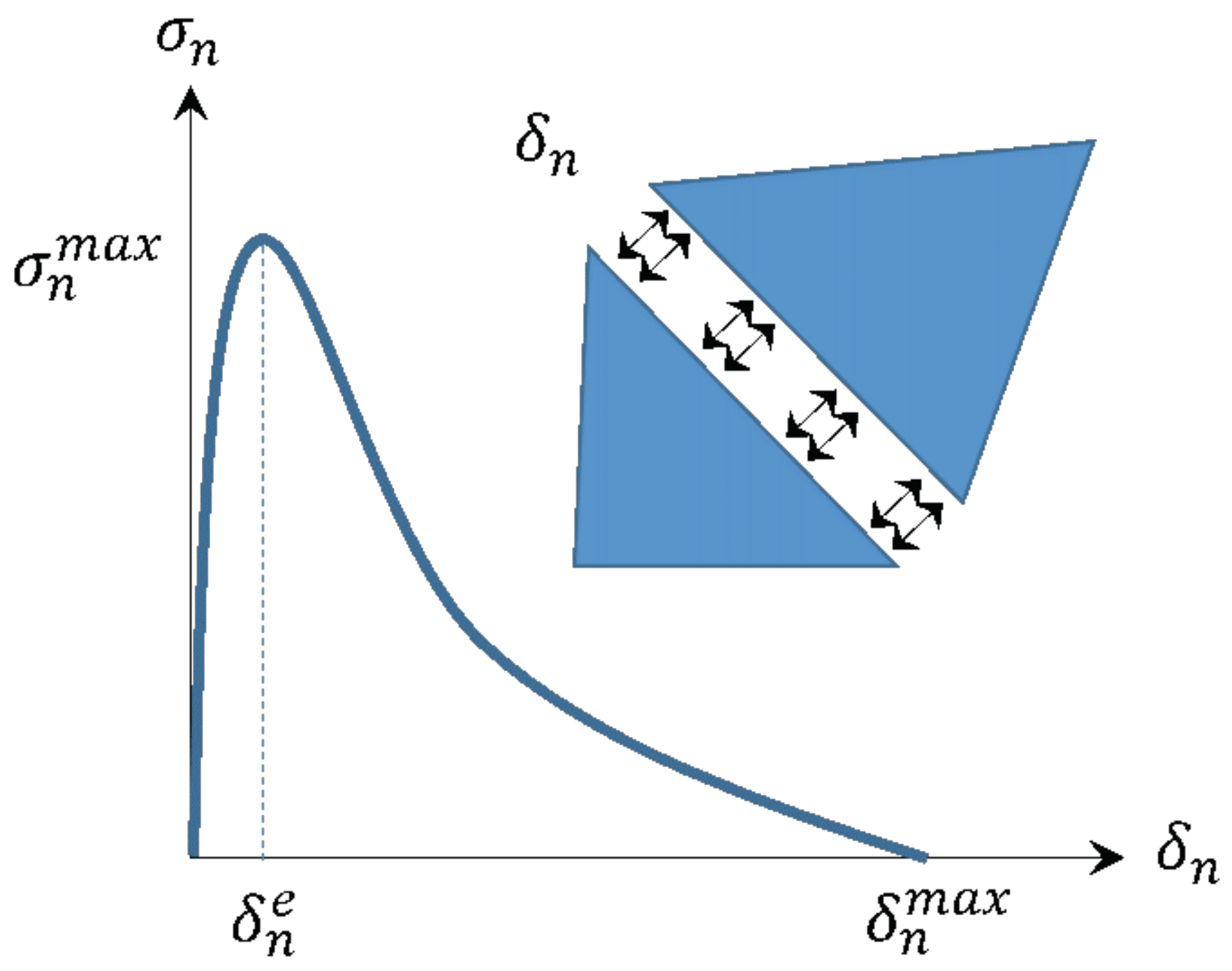
2. HOSS Simulations and FDEM Model for Dynamic Fracture

HOSS is a FDEM code that was specifically designed to simulate problems involving fracture and fragmentation processes in a diverse range of materials [54]. Within the FDEM framework [50], finite element method solutions are combined with the discrete element method to simulate dynamic fracture. In this setting, solid domains are discretized using finite elements in order to describe their deformation and stresses. Finite rotations and finite displacements are assumed a priori. That is, we do not make prior assumptions of small deformations or small rotations in our FDEM numerical formulation. To resolve fracture and contact processes between different parts, we allow material interaction along the boundaries of finite elements. The finite element deformation kinematics is handled via a multiplicative decomposition-based finite strain formulation [42]. The fracture model used in this present work is the combined single and smeared crack model introduced by Munjiza [49]. The contact interaction is resolved using the triangle-versus-point algorithm, which is the 2D extension of the tetrahedron-versus-point algorithm [51].

In the FDEM formulation, the interface between any two finite elements consists of non-linear springs that model tensile and shear behavior. These springs can hold a maximum tensile stress equal to the tensile strength of the material ${\sigma }_n^{max}$ and a maximum shear stress that is based on a combination of the cohesion (Mohr-Coulomb model) and the frictional strength [68]. Figure 1 presents a schematic representation of stress-displacement curve, which shows the response of the springs between the elements accounting for opening (i.e., the normal response). We note that the HOSS simulations have both normal springs and shear springs present between all elements, but in Figure 1 we have only shown normal springs for convenience. Hence the finite elements can move apart or open (via normal springs), and slide against each other (via shear springs). The non-linear response of the shear springs is similar in shape to that of the normal springs, although parameterized slightly differently to properly account for degradation in shear directions. In the region $0\le {\delta }_n\le {\delta }_n^e$ and $0\le \sigma \le {\sigma }_n^{max}$, the springs undergo non-linear elastic behavior without any damage. Beyond the elastic limit, ${\delta }_n^e<{\delta }_n<{\delta }_n^{max}$, strain softening is assumed that mimics degradation in strength. When ${\delta }_n>{\delta }_n^{max}$, these springs are broken and cannot bear any load.

In this work, HOSS has been used to simulate brittle fracturing under uniaxial tensile loading conditions in concrete samples containing 20 randomly placed pre-existing cracks. The loading is provided by displacement control. The sample size was set to 2 m wide and 3 m high. A schematic of the numerical simulation setup is shown in Figure 2. The bottom edge of the sample is fixed and the top edge of the sample moves upwards with a constant velocity of 0.3 m/s. This boundary condition corresponds to a strain rate of 0.1 ${\mathrm{s}}^{-1}$. The lengths of pre-existing cracks was set to 0.3 m. Random sampling for crack placement and crack orientation selection is based on a discrete uniform distribution. The model domain is divided in to a grid of size 0.5 m × 0.5 m resulting in 24 grid cells. A grid cell is chosen without replacement to randomly place a crack. This is done to ensure that the pre-existing defects do not overlap. This step is repeated until we place all the 20 cracks of size 0.3 m in the model domain. The center of the crack coincides with the center of the grid. The crack orientation was randomly selected between 0, 60, and 120 degrees with respect to horizontal. Other parameters used include: sample density of 2500 kg/m³, Young’s modulus of 22.6 GPa, shear modulus of 9.1 GPa, and a Poisson’s ratio of 0.242. The mesh used in this work contains constant strain triangles with an average size of 0.01 m. This corresponds to a total of approximately 160,000 cells and 480,000 edges. The tensile strength of the material was set to 8 MPa. Mohr-Coulomb fracture model is implemented at the interface of the triangular finite elements, which describes the strength of the material in shear. The shear cohesion and the internal angle of friction were set at 24 MPa and 31 degrees respectively. 190 high-fidelity HOSS simulations were performed for different initial crack locations and orientations. Loading conditions, material parameters, and domain dimensions are unchanged for all 190 HOSS simulations. HOSS output was stored at every 2000 time steps with each time-step being ${10}^{-8}$ s. Each simulation took about 4 h of computation time on 400 processors. At the point of failure, the material is unable to bear further load resulting in Mode I failure. The sample is considered as failed when a set of fractures connect the two opposite boundaries of the domain.

HOSS has been previously validated for several applications and it is shown to be reliable [49,69,70,71]. Validation of HOSS that may be of particular interest is cases addressing the brittle failure of geomaterials. In this regard, HOSS has modeled split Hopkinson bar experiments on granite [69], producing excellent comparison to experimental data in addition to capturing the complex crack networks that evolve during high-rate loading conditions. Furthermore, HOSS has directly compared simulated and experimental fracture patterns in granite samples under low-rate compressive loads [71]. HOSS simulated experimental fracture patterns in shale have also been compared with promising results in Carey et. al. [70]. Based on this previous validation work, we aim to develop surrogate models that can emulate HOSS. For large components, HOSS simulations can be computationally costly. This can become important when many simulations are required, for example in uncertainty quantification or sensitivity studies. Surrogate models that can emulate HOSS could quickly provide large sets of data for such investigations.

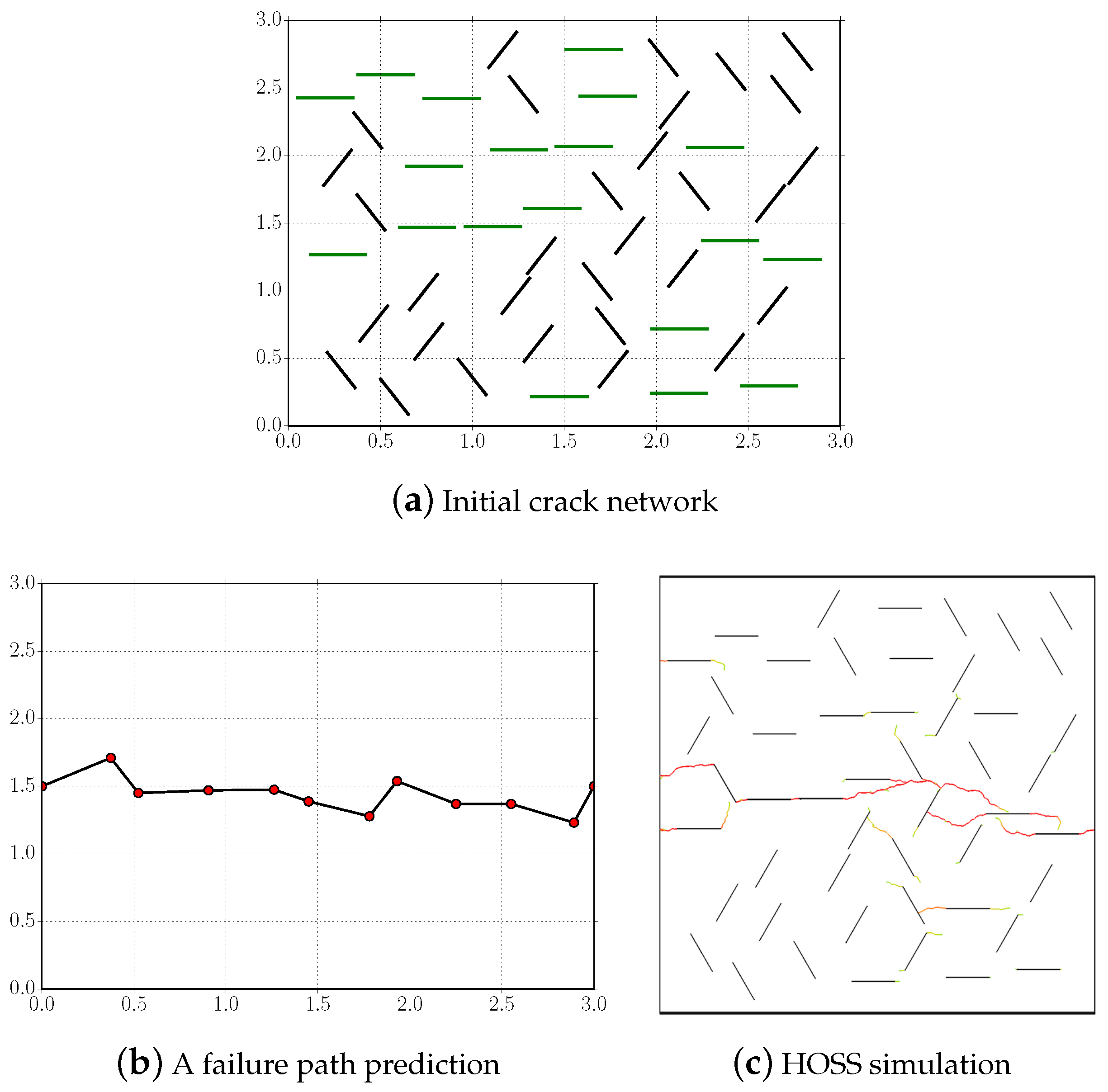
3. An Algorithm to Estimate Failure Paths

In this section, we provide a detailed description of our proposed method to estimate failure paths. The goal is to find the possible pathways to failure using weighted shortest path algorithms [Chapter-3] [72] based on initial crack configuration. Figure 3 provides a graph based pictorial description of failure paths and Algorithm 1 summarizes the proposed method to estimate failure paths. In our method, we assume graph nodes to be crack tips and graph edges are line segments connecting these tips. At initial times, when the system is not loaded, our premise is that pre-existing cracks are not connected to each other. In the graph theory representation, this implies that there is no connectivity between edges. As the system is being loaded, pre-existing cracks grow and intersect with other cracks leading to the formation of new edges. The schematic of all the possible paths connecting one side of the domain to another side at the time of failure for an initial pre-existing crack configuration is shown in Figure 3. In fracture mechanics, there are three different modes of fracture: Mode I, Mode II, and Mode III [1,73,74]. Mode I corresponds to crack opening mode, which is the most common mode in fracture toughness testing of brittle materials [5,6,75]. Mode II is in-plane shear and Mode III is out-of-plane shear or tearing mode. The proposed method focuses on Mode I failure and while it is possible to extend the algorithm to consider other failure modes, it is outside the scope of this study.

Failure of brittle and quasi-brittle materials under Mode I typically starts with the development of a FPZ around the crack tip [2,3,76]. The FPZ is a region of high stress around the crack tip where damage accumulates as the crack propagates over time. At a given instant of time, length of the FPZ is directly proportional to the length of the crack [77]. Very small micro-cracks are formed in the vicinity of the crack tip as stresses are the highest in this region. As the crack advances over time, the micro-cracks within the FPZ coalesce to become a single entity. This results in the formation of larger cracks. Larger cracks are bound to have a stable crack growth compared to smaller cracks [73]. Once these long cracks are formed, they grow rapidly with minimal additional loading. Therefore, the possible failure paths correlates directly with FPZs, which is the basis for our proposed method.

Various crack interaction and coalescence rules (e.g., alignment rules, combination rules) have been proposed in literature [77,78,79,80,81] based on fracture mechanics analysis. Wang and co-authors [77] provide FPZ-based rules for multiple crack interaction and coalescence. In these rules, crack interaction and coalescence are based on the Euclidean distance between cracks tips (for e.g., see [Table-1] [81]). We note that these rules have been widely adopted in brittle and quasi-brittle failure analysis (for e.g., see [Equation-1 and Sec-1] [77]) and fitness-for-service codes [Table-1 and Introduction] [81]. In this paper, we take advantage of these crack interaction and coalescence rules that are built on sound fracture mechanics underpinnings to develop FPZ-based graph surrogate model to estimate failure paths.

The first step of the proposed method is to identify the cracks which are likely to coalesce. In order to achieve this, we find pre-existing cracks that are orthogonal to the tensile loading. These correspond to all 0-degree angle cracks in the domain (as the orientation of these cracks is best suited for Mode I opening). It is expected that they will have the fastest growth and we assume that the failure path will include one or more 0-degree angle cracks. For each tip of these 0-degree angle cracks, we calculate ten nearest crack tip neighbors using a kNN algorithm [82] with $k=10$ and their respective Euclidean distances. These nearest neighbor crack tips can belong to either 0-degree, 60-degree or a 120-degree crack. Among these ten nearest crack tip neighbors, we identify the ones that could interact or coalesce with the horizontal cracks. Crack interaction or crack coalescence occurs if the FPZ of two neighboring cracks overlap. That is, if the Euclidean distance of a nearest neighbor is less than the length of FPZ, then we assume that the neighboring cracks are going to coalesce to form a larger crack. In the graph based representation of failure, we form new edges by joining the crack tips that have overlapping FPZs. The size of the FPZ, $l_{12}$, is given as [77]:

$$\begin{array}{c}\hfill l_{12}\propto {\left(\frac{\sigma }{{\sigma }_y}\right)}^2(l_1+l_2)\end{array}$$

(1)

where $\sigma$ and ${\sigma }_y$ are the applied and yield stresses of the material. $l_1$ and $l_2$ are the length of the interacting cracks. Herein, we assume that the size of FPZ to be 75% of $(l_1+l_2)$. Forsyth [83] was among the first to introduce Equation (1) to calculate the size of FPZ. We note that this equation has been used in various experimental and modeling works in literature [83,84,85,86].

Once we have identified the potential coalescing cracks, we next identify the regions or zones of interest in which failure is likely to occur. It should be noted that there may be one or more potential failure zones in a specimen. However, in a realistic system only one of these failure paths will actually correspond to the sample’s complete failure. To identify this failure zone, we divide the entire domain into a set of non-overlapping rectangular zones. Let the total number of non-overlapping rectangular zones be equal to $\mathtt{NumZones}$. The width of the rectangular zone is equal to the width of the domain and its height is equal to $\frac{H}{\mathtt{NumZones}}$, where H is the height of the specimen. Then, we form a weighted undirected graph for the entire domain. This weighted graph contains graph nodes (which are crack tips), pre-existing edges, and newly formed edges. Preexisting edges representing initial cracks are given small edge weights, equal to ${10}^{-4}$. The rationale behind giving small edge weights to initial cracks is that, physically, there is a strong possibility for the failure path to traverse through these cracks. The weights of the newly formed edges are equal to their length. Once this weighted graph is formed, we find all the connected components in each non-overlapping rectangular zone. A connected component of a weighted undirected graph is a set of nodes such that each pair of nodes is connected by a path. The Depth First Search algorithm available in NetworkX [87] is used to identify connected components. After identifying them, we search for the non-overlapping rectangular zone which has maximal connected component. Here, the maximal connected component is defined as a connected component whose number of nodes is at least greater than or equal to the number of nodes in every other connected component in the graph. The maximal connected component is identified in order of size, number of 0-degree cracks, largest length, and location with respect to loading side of the domain (see step-18 in Algorithm 1).

Algorithm 1 Failure paths prediction algorithm for many-crack geometries using weighted graphs.

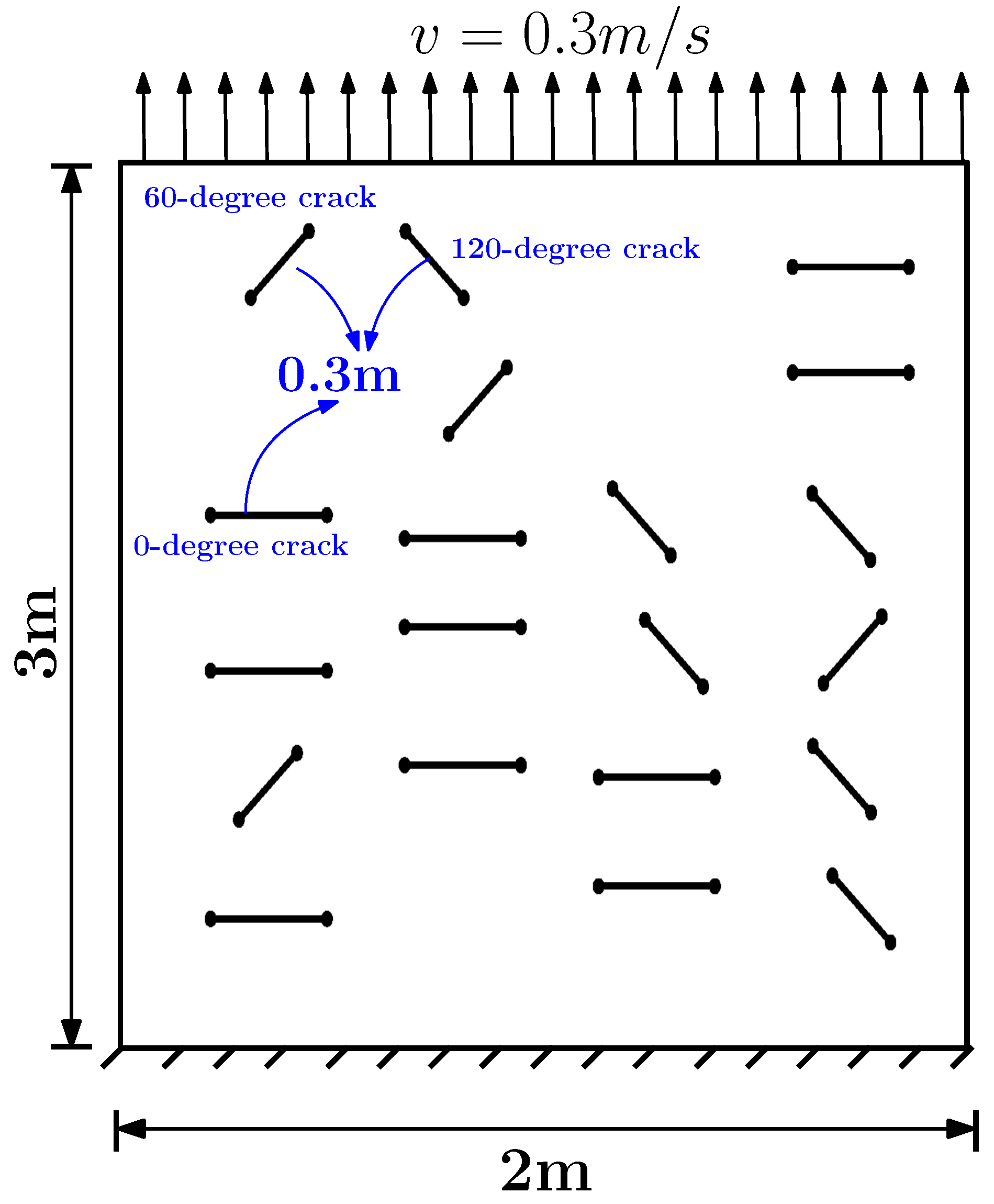
1: INPUT: Domain length; Initial coordinates of the crack tips; $\mathtt{NumZones}$: Total number of regions the domain is divided into (in-order to estimate zone of failure); Length of FPZ.

2: Identify the 0-degree angle cracks that are perpendicular to tensile loading.

3: for Each crack tip in the set of all 0-degree angle cracks: do

4:  Calculate ten nearest crack tip neighbors using kNN algorithm with $k=10$ and their respective Euclidean distances.

5:  Among these ten nearest crack tip neighbors, identify the ones that fall within the FPZ. These are determined as follows:

6:  for $i=1,2,\cdots ,10$: do

7:   if The Euclidean distance of an $i^{\mathrm{th}}$-nearest neighbor ≤ Length of FPZ: then

8:    Mark and store the $i^{\mathrm{th}}$-crack tip and the corresponding Euclidean distance.

9:   end if

10:  end for

11: end for

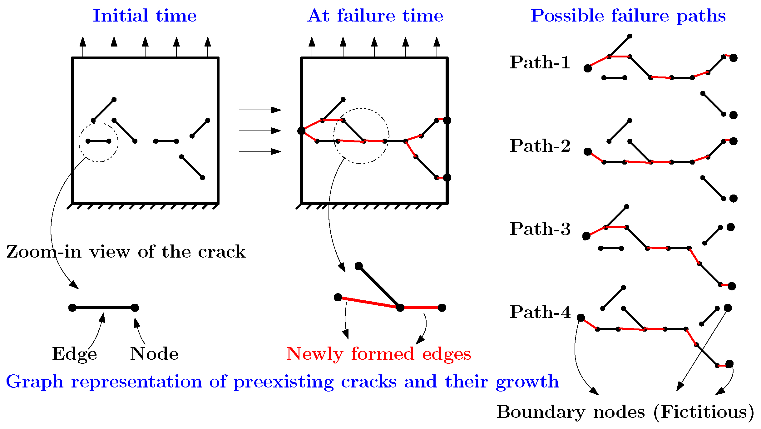
12: Form new edges by joining the crack tips that fall within the fracture process zone.

13: for $i=1,2,\cdots ,$ $\mathtt{NumZones}$: do

14:  Get and store the connected components in $i^{\mathrm{th}}$-zone.

15:  Get the total number of connected components, size of each connected component, and its length.

16:  Identify and store the 0-degree cracks present in these connected components.

17: end for

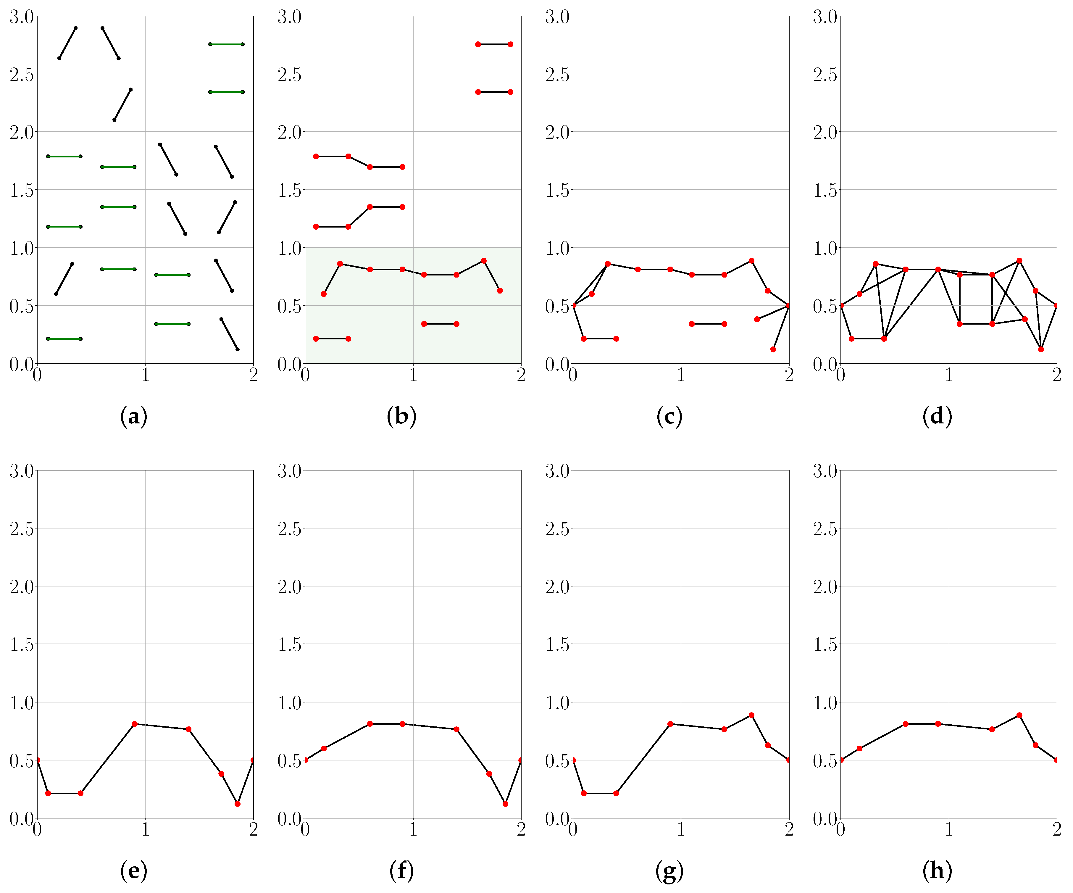
18: Identify the failure zone. This is accomplished as follows: First, we get the largest/maximal connected component in each zone using the Depth First Search algorithm. Second, if two or more zones contain connected components that are of same size, then we choose a connected component which has maximum number of 0-degree cracks. Third, if the above set of connected components contain same number of 0-degree cracks, then we choose the one which has the largest length. Length of a connected component is defined as the sum of edge weights. Finally, if they have the same length, then we choose the connected component which is closest to the loading side of the domain.

19: The goal is to detect failure paths along the length of sample, we introduce boundary nodes in the failure zone. Their location is given as follows: If the index of the failure zone is ‘i’, width of the domain is L, and H is the height of the domain; then the boundary nodes are located at $(0,\frac{(i-0.5)\times H}{\mathtt{NumZones}})$ and $(L,\frac{(i-0.5)\times H}{\mathtt{NumZones}})$

20: Create a weighted graph within the failure zone. To achieve this we do the following: We search for two nearest neighbors for each crack tip. Then, we connect these two nearest neighbors with the corresponding crack tip to form new edges. The weights for these newly formed edges are equal to Euclidean distance. Initial cracks within the failure zone are given small edge weights = ${10}^{-4}$. This is because, physically, there is a strong possibility for the failure path to traverse through the pre-existing cracks. Once we construct the edges and their weights, we form a weighted graph.

21: Next, we compute shortest paths within this weighted graph using Dijkstra’s method. The weighted shortest paths are calculated in two ways, both with and without the constraint that the path has to traverse through the identified connected component in the failure zone.

In the final step of the proposed method, we look for weighted shortest paths connecting the sides of the domain which are parallel to the tensile loading direction. First, we introduce boundary nodes in the failure zone and create a weighted undirected graph within this zone. New edges are constructed by connecting a given node to two of its nearest neighbors. As mentioned previously, the weights for these newly formed edges are equal to the Euclidean distance and initial cracks are given relatively small edge weights. Once a weighted graph is formed, we compute shortest paths from one boundary node to another boundary node. Analysis is performed with and without the constraint that the path has to traverse through the identified maximal connected component. Relaxing the above constraint gives more flexibility in identifying other possible paths (Section 5 discusses more on this aspect). Dijkstra’s algorithm [72] (Chapter-3) is used to compute the weighted shortest paths.

We note that Algorithm 1 is generic as there are no hard-coded values on the length of the cracks, specimen size, etc. In addition, the algorithm is not limited to only three crack orientations, and could consider continuously generated orientations. The only condition that the algorithm (see step-2) assumes is that the cracks are at a 0-degree angle. This condition can be relaxed by considering other pre-existing cracks that may be advantageously orientated for growth with respect to the loading conditions, and include such cracks in estimating the failure paths.

4. An Algorithm to Estimate Damage

For upscaling to continuum-scale constitutive models, statistical information that describes damage accumulated over time is needed. In this section, we provide an algorithm to estimate damage accumulation along failure paths from the HOSS simulation data. As mentioned in Section 2, within our FDEM framework, cracks are formed along the edges of the mesh elements. Opening and/or shearing between two elements is determined with multiple cohesive points, which are modeled as non-linear springs. For each pair of finite elements, we have a user specified number of non-linear springs. For our HOSS simulations, we have assumed four normal and four shear springs. The number four has been chosen because it has been used previously [69] and produced good results in comparison to experimental results with reasonable computational expense. Figure 1 shows a schematic of the stress-displacement curve, which is representative of each cohesive point’s normal response. This response represents reversible elastic damage and softening due to damage growth and coalescence. As the crack grows, the interfacial springs go through a non-linear elastic regime, where the maximum elastic opening (or shearing) of the spring is ${\delta }_n^e$. The total maximum opening (or shearing) of the spring is ${\delta }_n^{max}$. Between the maximum elastic opening and total max displacement is the strain softening regime. The area under this portion of the curve corresponds to the strain energy density (i.e, energy per length) dissipated during damage evolution. The maximum stress that the spring can withstand in either tension (opening) or shearing is represented by ${\sigma }_n^{max}$. Damage accumulated per unit length between two finite elements is evaluated based on the strain of the springs that exceed ${\delta }_n^e$. This value ranges from zero to one. Zero damage value corresponds to undamaged springs (${\delta }_n\le {\delta }_n^e$) and damage value of one corresponds to completely broken springs $({\delta }_n>{\delta }_n^{max})$.

We use a non-parametric approach for determining the evolution of damage. This is achieved by constructing a confidence interval over time. 150 HOSS simulations are used for training and 40 simulations are used for testing the damage evolution model. Let t be the time index, our 95% confidence interval for damage at t is given by $\left(D_L^{\left(t\right)},D_U^{\left(t\right)}\right)$. The damage $D^{\left(t\right)}$ is the accumulated damage along the failure path as a function of time in our damage evolution surrogate model. Accumulated damage along the failure path is calculated by summing the growth of all propagating cracks at every time-step within the HOSS simulation time. $D_L^{\left(t\right)}$ and $D_U^{\left(t\right)}$ correspond to lower and upper estimate on damage at a given instance of time. We use bootstrapping [88,89] to estimate $D_L^{\left(t\right)}$, $D_U^{\left(t\right)}$, and mean damage $\overline{D_M^{\left(t\right)}}$ from our training data. If a parametric distribution on the damage is desired, then one can prescribe a Gaussian distribution using the quantities, $\overline{D_M^{\left(t\right)}}$, $D_L^{\left(t\right)}$ and $D_U^{\left(t\right)}$ as follows, $D_M^{\left(t\right)}\sim \mathcal{N}\left(\overline{D_M^{\left(t\right)}},{\sigma }^{\left(t\right)}\right)$. Mean and variance of the distribution being $\overline{D_M^{\left(t\right)}}$ and ${\sigma }^{\left(t\right)}$, where ${\sigma }^{\left(t\right)}=max\left(0.5\ast \left(\overline{D_M^{\left(t\right)}}-D_L^{\left(t\right)}\right),0.5\ast \left(D_U^{\left(t\right)}-\overline{D_M^{\left(t\right)}}\right)\right)$. Although we have not made it explicit, most damage occurs within our predicted path to failure. Of course other cracks will have some propagation, but in most cases failure is driven by a dominant fracture pathway. For testing, to show that our confidence interval captures the damage from the test set, we calculate empirical coverage over time. Empirical coverage represents the fraction of test cases that fall within our estimated confidence interval at anytime. Mathematically, it is defined as,

$$\frac{1}{N_T^{\left(t\right)}}\sum _{j=1}^{N_T^{\left(t\right)}}{\mathbb{I}}_{D_j\in \left(D_L^{\left(t\right)},D_U^{\left(t\right)}\right)}$$

where $N_T^{\left(t\right)}$ is the test set data at time t and $D_j$ is one such data point of damage in our test set. ${\mathbb{I}}_{D_j\in \left(D_L^{\left(t\right)},D_U^{\left(t\right)}\right)}$ indicates if $D_j$ is in the confidence interval. The empirical coverage is one measure of how well our predicted confidence interval captures unseen data. In the next section, we provide results and compare them with HOSS simulation data.

5. Results

In this section, we present results of the proposed methods to estimate failure. Following are the inputs given to Algorithm 1 to calculate failure paths: width of the domain is equal to 2 m, height of the domain is equal to 3 m, $\mathtt{NumZones}$ = 3, initial crack tip coordinates, and length of FPZ = 0.45 m, which is quasi-brittle. We use 190 simulations to test the proposed method to estimate failure path for the 20 crack problem. In addition, we present a result for a configuration with 50 pre-existing cracks (whose crack tip coordinates are chosen randomly) to demonstrate its predictive capability.

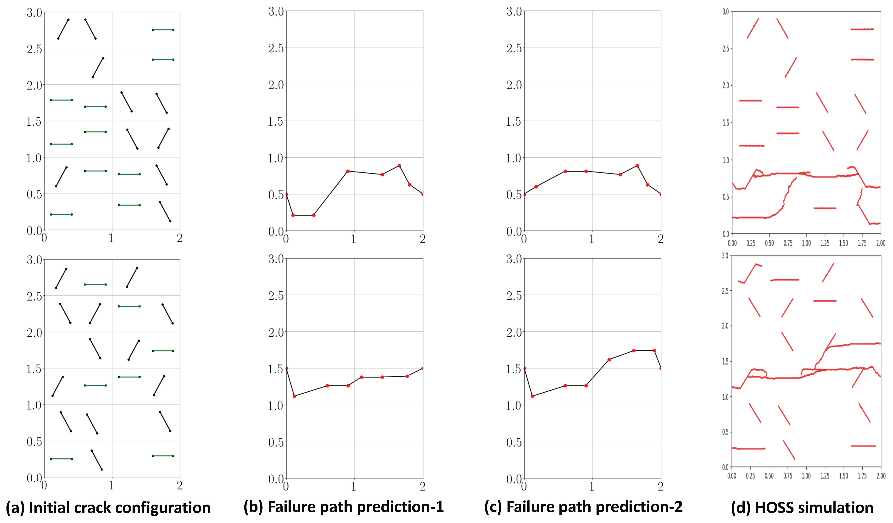
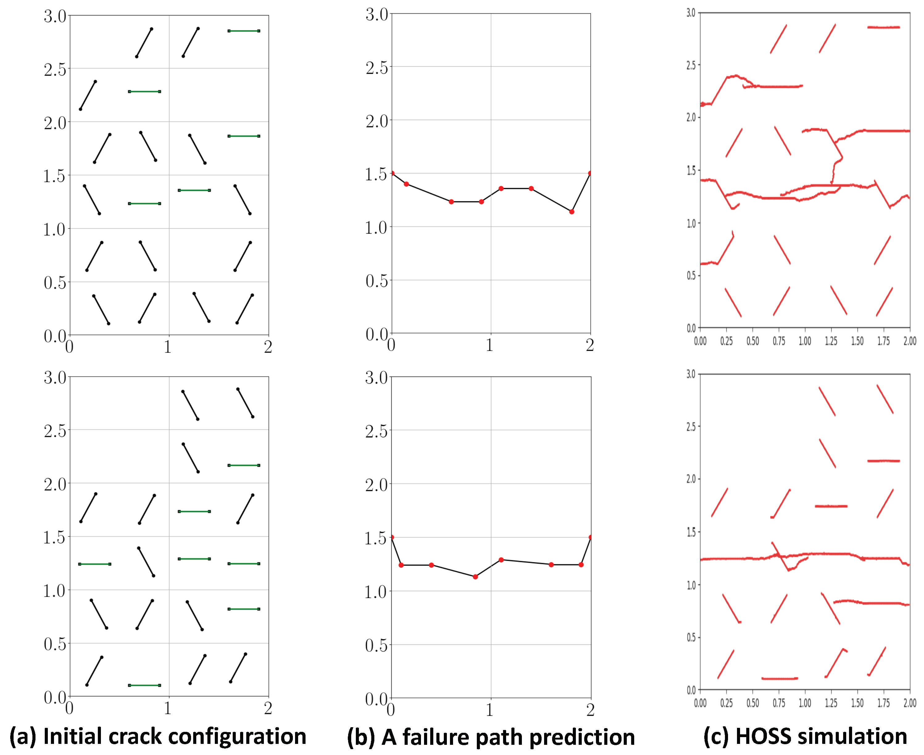
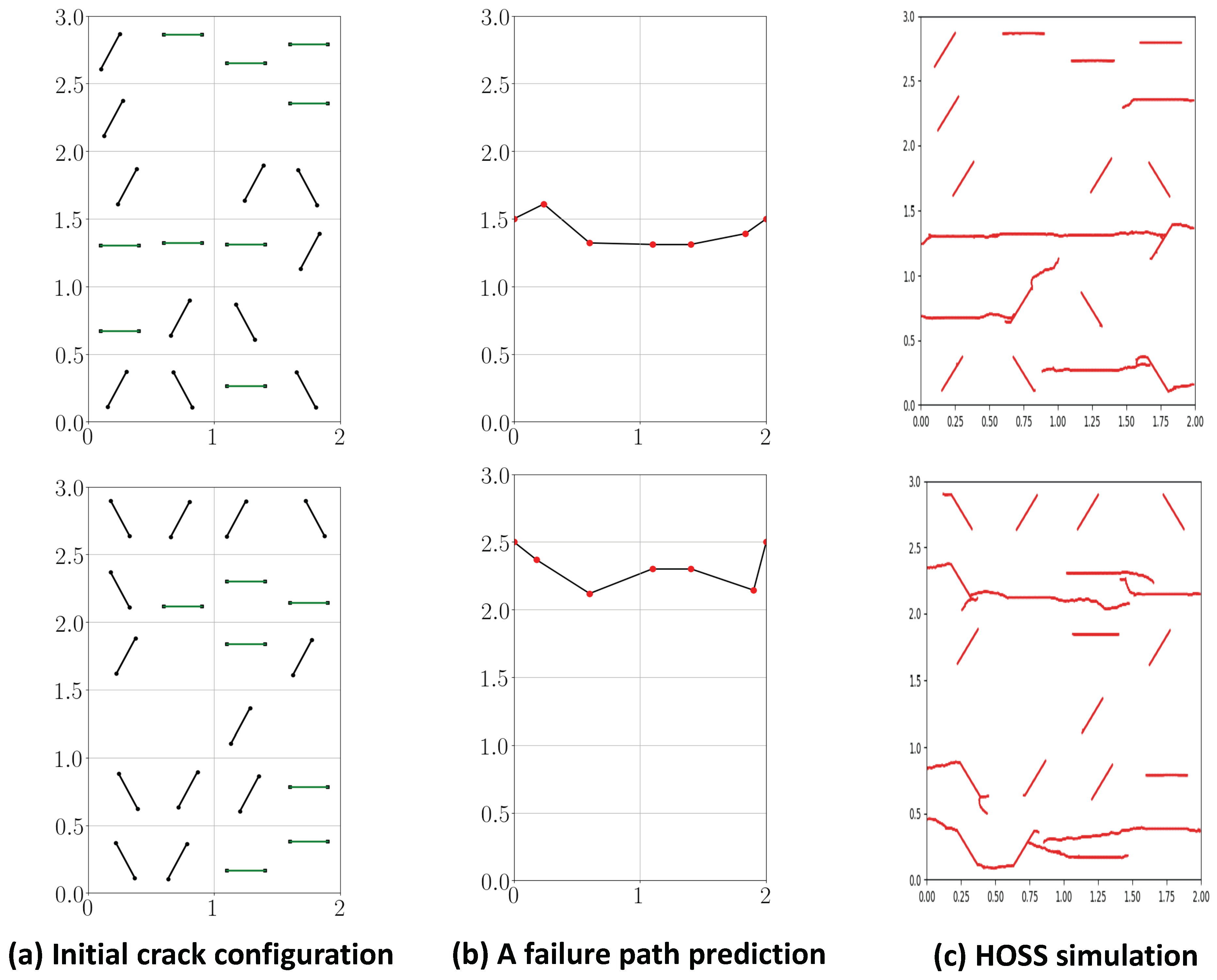
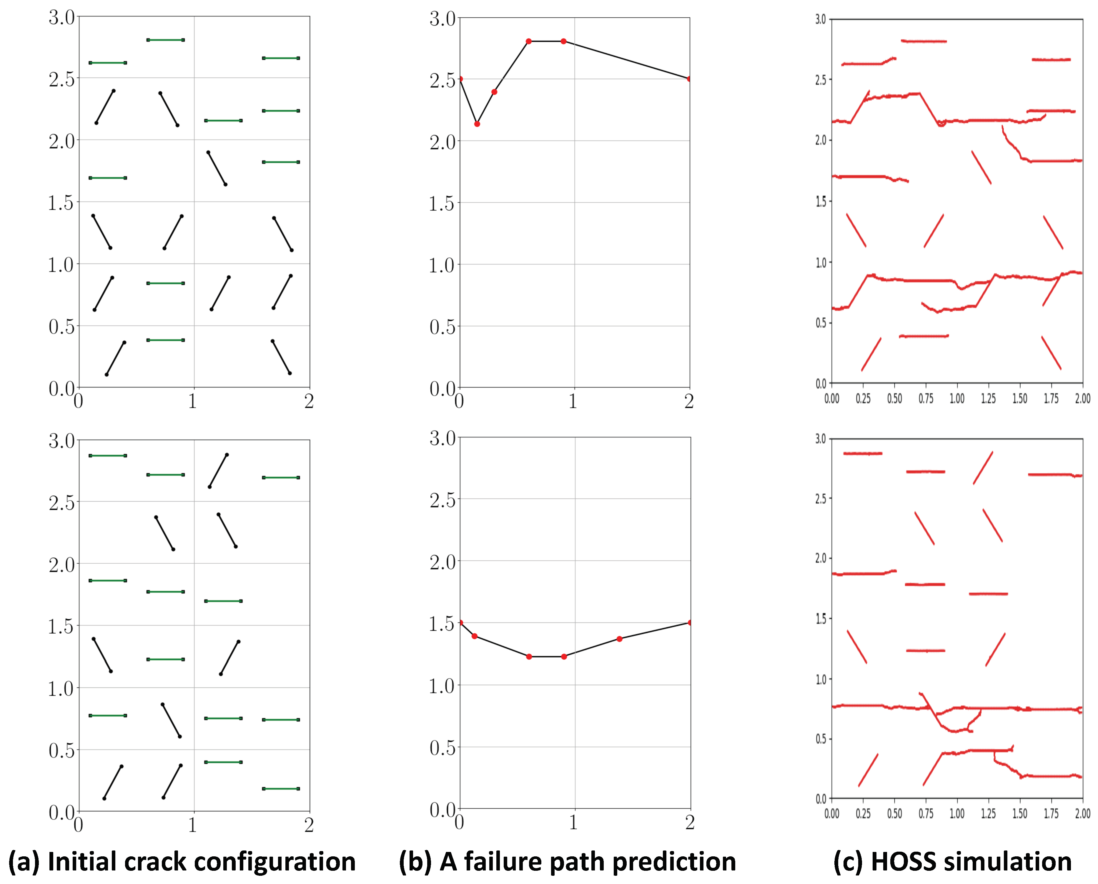
5.1. Estimating Failure Paths

Figure 4 provides a step-by-step description of the proposed method for estimating failure paths. First, we identify cracks that are perpendicular to the tensile loading. These are 0-degree cracks and are highlighted in green in Figure 4a. Second, we identify zone of failure, which is shown in light blue in Figure 4b. This corresponds to the region where failure occurs. As described in Section 3, we identify larger cracks that are formed after connecting pre-existing cracks that fall within the FPZ to determine failure zone. Third, we introduce boundary nodes in the failure zone (see Figure 4c). Fourth, we search for two nearest neighbors for each crack tip in the failure zone. Then, we form new edges with edge weights being the Euclidean distance. Fifth, we connect all the edges to form a weighted graph and look for failure paths connecting the boundary nodes (see Figure 4d). Finally, we compute all possible weighted shortest paths (see Figure 4e–h). The proposed method identified four possible shortest paths. Among the four paths two paths are of exact match (see Figure 5d) and other two are the next best match. Failure paths are computed with and without enforcing the constraint that the shortest path has to traverse through the maximal connected component. Herein, this constraint is enforced with some flexibility. Meaning that, we find shortest paths that contain at least one node to be present in the maximal connected component. This ‘soft’ enforcement of the constraint is done with the intention to capture multiple failure paths (if they exist).

Figure 5, Figure 6, Figure 7 and Figure 8 show examples for failure path prediction and comparison with HOSS simulations. When a possibility that multiple failure paths may exist, pinpointing an exact one is very hard. Moreover, constructing a metric or criterion for an exact match can be challenging. Given an initial crack configuration, a plausible measure to assess the accuracy of the proposed method is as follows: If the predicted failure path has at least 50% of the initial cracks or their crack tips to be within the HOSS failure path, then we say that the proposed method is a reasonable prediction of the simulated results. Figure 5 presents example results in which the graph theory approach predicted two equally likely failure paths for one initial crack configuration. Two different initial crack configurations are shown in Figure 5a. The cracks perpendicular to tensile loading are highlighted in green. Figure 5b,c show the multiple failure paths predicted by the graphs for each case. The HOSS predicted failure paths for both cases are provided in Figure 5d. From these figures, it can be inferred that the proposed method is able to predict multiple failure paths for a given initial crack configuration.

Figure 6 shows example results from the graph theory approach for cases where there was only one predicted failure path with comparison to results from HOSS. Figure 6a shows the initial crack configuration. Figure 6b shows the failure path prediction using the proposed method. Figure 6c shows the results obtained from the HOSS simulations. It should be noted that it is not always possible to predict all paths of failure. For example, the HOSS results shown in Figure 6c contain complex failure paths that could be considered two distinct pathways. However, our method provided only a single failure path. There are 43 out of 190 simulations where the graph approach has predicted a single failure path and matched perfectly with atleast one failure path of HOSS simulation. By perfect match, we mean that all of the initial cracks or crack tips in the graph predicted failure path are also in the HOSS predicted path.

Figure 7 shows example results from the graph theory approach for cases where there was only a partial match. Quantitatively, by partial match we mean atleast 50% of the initial cracks are in the failure paths in comparison to the HOSS simulations. Predictions that have more than 50% of the initial cracks in the failure paths and also have a zone of failure similar to that of HOSS are a total of 75 out of 190. Note that these 75 are separate from the previously mentioned 43 simulations. Figure 8 shows example scenarios where the proposed method failed to match the HOSS results. Predictions that fall in this category are the remaining 72 out of 190.

Table 1. Summary of the proposed method to estimate failure paths. Among various failure paths provided by the proposed method, if a failure path exactly matches the HOSS results, then we consider that as an accurate prediction. Meaning that, all the initial cracks or their crack tips identified by the proposed method fall within the dominant HOSS fracture path. If the proposed method predicts 50% of the initial cracks or their crack tips to be within the HOSS failure path, then we consider it as a reasonable prediction. A non-matching failure path is a scenario where the prediction of the proposed method is less than 50% match.

Scenario Description	Number of Simulations	% of Failure Path Match
Accurate prediction of failure path	43	100% match
Reasonable prediction of failure path	75	>50% match
Non-matching failure paths	72	<50% match
Total	190

summarizes the accuracy of the proposed method, which is the number of reasonably accurate predictions made by the Algorithm 1. Out of 190 simulation, the proposed method predicted the failure paths of 118 simulations with reasonable (50% of the failure path) or accurate prediction (100% of the failure path). The prediction accuracy of failure zones by the proposed method is 143 simulations out of 190 simulations. It should be noted that the time taken by the proposed method to predict a failure path is a couple of seconds, which is $\approx \mathcal{O}\left({10}^6\right)$ times less than a single HOSS simulation.

For Mode I loading, we can roughly determine the cases where there is a chance that the surrogate fails a priori. For example, if there are small number of 0-degree angle cracks or if the 0-degree angle cracks are far away from each other, then the Euclidean distance between a pair of 0-degree angle cracks is greater than the length of FPZ. Hence, there is no interaction between the pair of 0-degree angle cracks, and it will be more difficult for the graph-based surrogate model to reliably predict the failure pathway. This highlights a need for improved feature engineering, perhaps including some information about long-range interactions between pre-existing cracks.

Figure 9 shows the failure path prediction for an initial configuration with 50 pre-existing cracks. This figure describes the application of the proposed method for estimating failure paths for larger number of cracks in the domain. The process to predict failure paths is the same as the 20 crack scenario. Figure 9b shows a failure path prediction, which agrees with HOSS results (see Figure 9c).

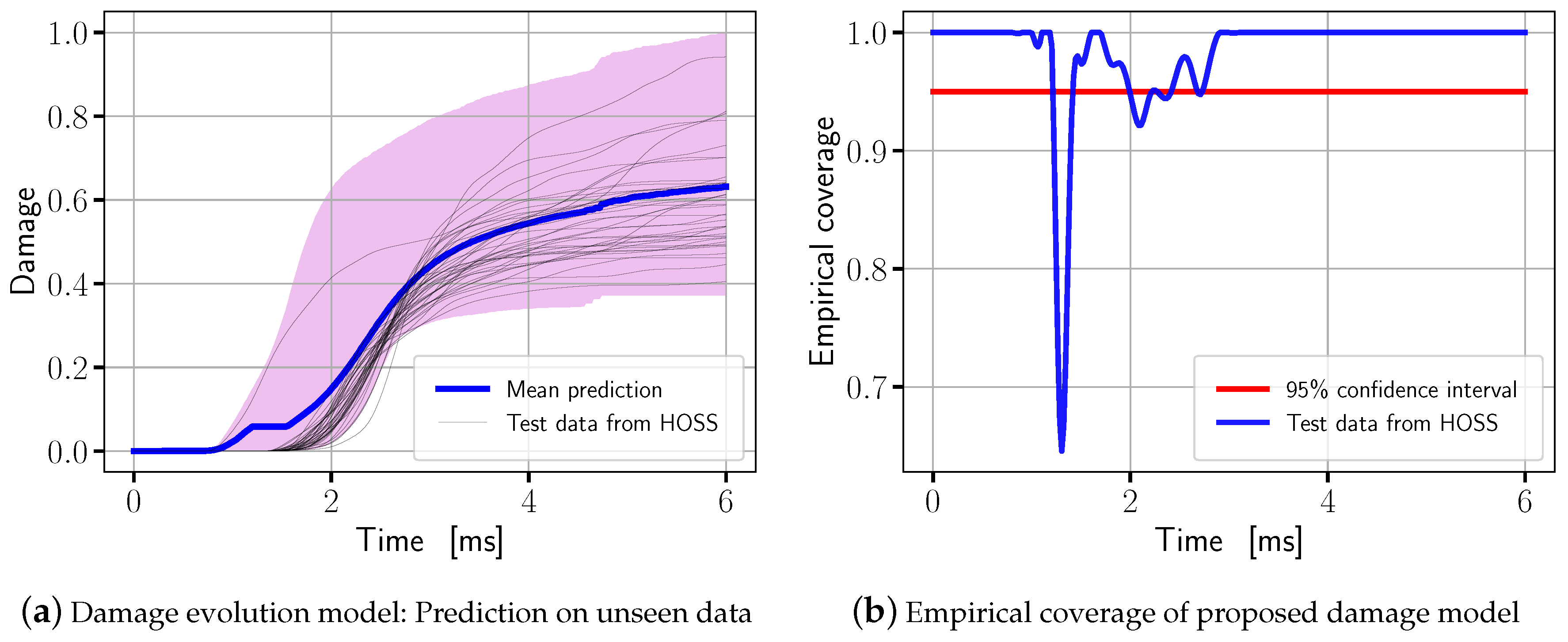
5.2. Estimating Damage Along the Failure Paths

Figure 10a shows the estimated damage evolution vs time, confidence interval, and prediction on unseen data. In this figure, the mean estimated damage $\overline{D_M^{\left(t\right)}}$ is shown with a blue line. The magenta region shows the damage confidence interval $\left(D_L^{\left(t\right)},D_U^{\left(t\right)}\right)$, which is constructed based on the method discussed in Section 4. The test data from HOSS simulations are shown in gray lines. Figure 10a shows that our confidence interval captures the damage from the test set.

Figure 10b provides the corresponding empirical coverage of the proposed surrogate model for damage. The blue line corresponds to the empirical coverage on the test dataset from HOSS. The red line corresponds to 95% confidence interval. As discussed in Section 4, empirical coverage is a measure of how well our predicted confidence interval captures unseen data. From this figure, we see that we are able to capture more than 90% of the test data over time except for a small region around time 1.75 ms where we under cover (this is because the cracks along the failure path start to grow around this time).

Macro-scale models can take advantage of the proposed methodology as follows: The proposed surrogate models provide statistics on the micro-scale damage evolution for each representative volume element (RVE). This statistical information obtained from the surrogate models is used in calculating macro-scale effective moduli. Specifically, the elastic moduli are degraded using probability distribution functions that describe the evolving lengths and orientations of all the micro-cracks within a RVE. The prediction accuracy (>90%) of the damage evolution surrogate model implies that the proposed method can be used to develop probability density functions. As the surrogate models are trained based on HOSS simulations, they contain crack interaction effects. Such interaction will ultimately impact the evolution of crack lengths and their orientations during tensile loading. Hence, this micro-crack interaction information can be incorporated into the effective moduli through the surrogates during the upscaling process. This implies that the material response we obtain at macro-scale scale includes crack interactions at micro-scale, which are typically lost if one employs traditional mechanistic or homogenization approaches [57,66,67,90]. An example of an upscaling method, which could make use of the proposed surrogate models to calculate effective elastic moduli, is described in reference [91].

6. Conclusions

Predicting damage evolution and when failure occurs is important to accurately predict the overall material response. This includes accounting for degraded material properties as damage accumulates and when and where failure of the specimen or part occurs, for example, which elements or cells will fail first. Providing such information is of great interest to the fracture and infrastructure maintenance communities. In addition, estimating likely failure paths and accumulated damage along the failure path is an important aspect for upscaling micro-scale models to macro-scale models. FDEM models and multi-physics numerical tools like HOSS are highly-accurate to simulate various stages of brittle fracture propagation. However, HOSS is data-intensive and computationally expensive. Moreover, scaling to larger and more complex problems is often computationally prohibitive with computational tools such as HOSS. This is due to the difference in length scales associated with small fractures and bulk material sizes. In this paper, we provided algorithms to address these aspects that are $\approx \mathcal{O}\left({10}^6\right)$ faster than high-fidelity simulations to estimate key QoIs for brittle fracture such as failure paths, failure zones, and damage along failure. Hence, the proposed methodology is ideal for usage in comprehensive uncertainty quantification studies.

The proposed failure path method was compared against high-fidelity HOSS simulations. From this comparison, we found that out of 190 simulations, the proposed method predicted failure paths of 118 simulations with reasonable accuracy (greater than 50% of initial cracks in the failure path) and zone of failure of 143 simulations with 100% accuracy. Damage along the failure path was estimated using a non-parametric approach. The damage evolution model was obtained by constructing a 95% confidence interval over time. 150 HOSS simulations were used to develop the damage evolution model and the remaining 40 simulations are used for testing. Bootstrapping was used to estimate lower and upper bounds for damage. Empirical coverage was used as a metric to understand the accuracy of the proposed damage evolution model. Empirical coverage tells us the fraction of test cases that falls within our estimated confidence interval at anytime. From empirical coverage results, it can be concluded that our confidence interval captures the damage from the test dataset with an accuracy greater than 90%. Damage is the key QoI for upscaling HOSS information to continuum codes such as FLAG. This is because continuum-scale models need effective moduli, which is a function of damage accumulated over time at micro-scale. Since the discrete crack network cannot be accounted for in continuum models, exact locations of the failure pathways becomes less important. The proposed damage model which takes into account the crack interaction effects provides such micro-scale information with high accuracy for simulating damage at larger-scales. The limitation of the proposed methods is that it is applicable only for Mode I failure at low-strain rates. Extensions to higher-strain rates and other modes of failure will be considered in our future works. Lastly, our method can be coupled with other machine learning and graph-based methods [92,93,94,95] for increased accuracy of failure paths prediction, which is our future work.

References

1. Bažant, Z.P.; Planas, J. Fracture and Size Effect in Concrete and Other Quasibrittle Materials; CRC Press: Boca Raton, FL, USA, 1998. [Google Scholar]
2. Petersson, P.-E. Crack Growth and Development of Fracture Zones in Plain-Concrete and Similar Materials. Ph.D. Thesis, Lund Institute of Technology, Lund, Sweden, 1981. [Google Scholar]
3. Brooks, Z. Fracture Process Zone: Microstructure and Nanomechanics in Quasi-Brittle Materials. Ph.D. Thesis, Massachusetts Institute of Technology, Cambridge, MA, USA, 2013. [Google Scholar]
4. Veselý, V.; Rǒutil, L.; Keršner, Z. Structural geometry, fracture process zone and fracture energy. In Proceedings of the Fracture Mechanics of Concrete and Concrete Structures, Catania, Italy, 17–22 June 2007. [Google Scholar]
5. Freiman, S.W.; Mecholsky, J.J., Jr. The Fracture of Brittle Materials: Testing and Analysis; John Wiley & Sons, Inc.: Hoboken, NJ, USA, 2012. [Google Scholar]
6. Lamon, J. Brittle Fracture and Damage of Brittle Materials and Composites: Statistical-Probabilistic Approaches; Elsevier: Oxford, UK, 2016. [Google Scholar]
7. Hyman, J.D.; Martínez, J.J.; Viswanathan, H.S.; Carey, J.W.; Porter, M.L.; Rougier, E.; Karra, S.; Kang, Q.; Frash, L.; Chen, L.; et al. Understanding hydraulic fracturing: A multi-scale problem. Philos. Trans. R. Soc. Lond. Ser. A Math. Phys. Sci. 2016, 374, 20150426. [Google Scholar] [CrossRef] [PubMed]
8. Mudunuru, M.K.; Karra, S.; Makedonska, N.; Chen, T. Sequential geophysical and flow inversion to characterize fracture networks in subsurface systems. Stat. Anal. Data Min. ASA Data Sci. 2017, 10, 326–342. [Google Scholar] [CrossRef] [Green Version]
9. Mudunuru, M.K.; Karra, S.; Harp, D.R.; Guthrie, G.D.; Viswanathan, H.S. Regression-based reduced-order models to predict transient thermal output for enhanced geothermal systems. Geothermics 2017, 70, 192–205. [Google Scholar] [CrossRef] [Green Version]
10. Noor, A.K.; Zarchan, P. (Eds.) Structures Technology for Future Aerospace Systems, Volume 188 of Progress in Astronautics and Aeronautics; Aerospace Press: Los Angeles, CA, USA, 2000. [Google Scholar]
11. Rice, J.R. Mathematical analysis in the mechanics of fracture. Fract. Adv. Treatise 1968, 2, 191–311. [Google Scholar]
12. Rice, J.R.; Thomson, R. Ductile versus brittle behaviour of crystals. Philos. Mag. A J. Theor. Appl. Phys. 1974, 29, 73–97. [Google Scholar] [CrossRef]
13. Hutchinson, J.W. Plastic stress and strain fields at a crack tip. J. Mech. Phys. Solids 1968, 16, 337–342. [Google Scholar] [CrossRef]
14. Hutchinson, J.W. Singular behaviour at the end of a tensile crack in a hardening material. J. Mech. Phys. Solids 1968, 16, 13–31. [Google Scholar] [CrossRef]
15. Hutchinson, J.W.; Suo, Z. Mixed mode cracking in layered materials. In Advances in Applied Mechanics; Academic Press Inc.: San Diego, CA, USA, 1991; Volume 29, pp. 63–191. [Google Scholar]
16. Xu, X.-P.; Needleman, A. Numerical simulations of fast crack growth in brittle solids. J. Mech. Phys. Solids 1994, 42, 1397–1434. [Google Scholar] [CrossRef]
17. Li, F.Z.; Shih, C.F.; Needleman, A. A comparison of methods for calculating energy release rates. Eng. Fract. Mech. 1985, 21, 405–421. [Google Scholar] [CrossRef]
18. Buehler, M.J.; Abraham, F.F.; Gao, H. Hyperelasticity governs dynamic fracture at a critical length scale. Nature 2003, 426, 141. [Google Scholar] [CrossRef]
19. Ravi-Chandar, K.; Yang, B. On the role of microcracks in the dynamic fracture of brittle materials. J. Mech. Phys. Solids 1997, 45, 535–563. [Google Scholar] [CrossRef]
20. Desroches, J.; Detournay, E.; Lenoach, B.; Papanastasiou, P.; Pearson, J.R.A.; Thiercelin, M.; Cheng, A. The crack tip region in hydraulic fracturing. Proc. R. Soc. Lond. Ser. A Math. Phys. Sci. 1994, 447, 39–48. [Google Scholar] [CrossRef]
21. Griffith, A.A. The phenomena of rupture and flow in solids. Philos. Trans. R. Soc. Lond. A 1921, 221, 163–198. [Google Scholar] [CrossRef]
22. Irwin, G.R. Analysis of stresses and strains near the ends of a crack traversing a plate. J. Appl. Mech. 1957, 24, 361–364. [Google Scholar]
23. Barenblatt, G.I. The mathematical theory of equilibrium cracks in brittle fracture. Adv. Appl. Mech. 1962, 7, 55–129. [Google Scholar]
24. Dugdale, D.S. Yielding of steel sheets containing slits. J. Mech. Phys. Solids 1960, 8, 100–104. [Google Scholar] [CrossRef]
25. Needleman, A. An analysis of tensile decohesion along an interface. J. Mech. Phys. Solids 1990, 38, 289–324. [Google Scholar] [CrossRef]
26. Beltz, G.E.; Rice, J.R. Dislocation nucleation versus cleavage decohesion at crack tips. In Modeling the Deformation of Crystalline Solids; Metallurgical Society of AIME: Englewood, CO, USA, 1991; pp. 457–480. [Google Scholar]
27. Xu, X.-P.; Needleman, A. Void nucleation by inclusion debonding in a crystal matrix. Model. Simul. Mater. Sci. Eng. 1993, 1, 111. [Google Scholar] [CrossRef]
28. Pandolfi, A.; Krysl, P.; Ortiz, M. Finite element simulation of ring expansion and fragmentation: The capturing of length and time scales through cohesive models of fracture. Int. J. Fract. 1999, 95, 279–297. [Google Scholar] [CrossRef]
29. Freed, Y.; Banks-Sills, L. A new cohesive zone model for mixed mode interface fracture in bimaterials. Eng. Fract. Mech. 2008, 75, 4583–4593. [Google Scholar] [CrossRef]
30. Park, K.; Paulino, G.H.; Roesler, J.R. A unified potential-based cohesive model of mixed-mode fracture. J. Mech. Phys. Solids 2009, 57, 891–908. [Google Scholar] [CrossRef]
31. De Borst, R. Fracture in quasi-brittle materials: A review of continuum damage-based approaches. Eng. Fract. Mech. 2002, 69, 95–112. [Google Scholar] [CrossRef]
32. Lisjak, A.; Grasselli, G. A review of discrete modeling techniques for fracturing processes in discontinuous rock masses. J. Rock Mech. Geotech. Eng. 2014, 6, 301–314. [Google Scholar] [CrossRef] [Green Version]
33. Miehe, C.; Welschinger, F.; Hofacker, M. Thermodynamically consistent phase-field models of fracture: Variational principles and multi-field FE implementations. Int. J. Numer. Methods Eng. 2010, 83, 1273–1311. [Google Scholar] [CrossRef]
34. Miehe, C.; Hofacker, M.; Welschinger, F. A phase field model for rate-independent crack propagation: Robust algorithmic implementation based on operator splits. Comput. Methods Appl. Mech. Eng. 2010, 199, 2765–2778. [Google Scholar] [CrossRef]
35. Ambati, M.; Gerasimov, T.; DeLorenzis, L. A review on phase-field models of brittle fracture and a new fast hybrid formulation. Comput. Mech. 2015, 55, 383–405. [Google Scholar] [CrossRef]
36. Verhoosel, C.V.; deBorst, R. A phase-field model for cohesive fracture. Int. J. Numer. Methods Eng. 2013, 96, 43–62. [Google Scholar] [CrossRef]
37. Borden, M.J.; Verhoosel, C.V.; Scott, M.A.; Hughes, T.J.R.; Landis, C.M. A phase-field description of dynamic brittle fracture. Comput. Methods Appl. Mech. Eng. 2012, 217, 77–95. [Google Scholar] [CrossRef]
38. Hakim, V.; Karma, A. Laws of crack motion and phase-field models of fracture. J. Mech. Phys. Solids 2009, 57, 342–368. [Google Scholar] [CrossRef] [Green Version]
39. Kuhn, C.; Müller, R. A continuum phase field model for fracture. Eng. Fract. Mech. 2010, 77, 3625–3634. [Google Scholar] [CrossRef]
40. Zienkiewicz, O.C.; Taylor, R.L.; Zhu, J.Z. The Finite Element Method: Its Basis and Fundamentals, 7th ed.; Butterworth-Heinemann, Elsevier Ltd.: Oxford, UK, 2013. [Google Scholar]
41. Mudunuru, M.K.; Nakshatrala, K.B. A framework for coupled deformation-diffusion analysis with application to degradation/healing. Int. J. Numer. Methods Eng. 2011, 89, 1144–1170. [Google Scholar] [CrossRef] [Green Version]
42. Munjiza, A.; Rougier, E.; Knight, E.E. Large Strain Finite Element Method: A Practical Course; John Wiley & Sons, Inc.: West Sussex, UK, 2015. [Google Scholar]
43. Portela, A.; Aliabadi, M.H.; Rooke, D.P. The dual boundary element method: Effective implementation for crack problems. Int. J. Numer. Methods Eng. 1992, 33, 1269–1287. [Google Scholar] [CrossRef]
44. Blandford, G.E.; Ingraffea, A.R.; Liggett, J.A. Two dimensional stress intensity factor computations using the boundary element method. Int. J. Numer. Methods Eng. 1981, 17, 387–404. [Google Scholar] [CrossRef]
45. Xu, C.; Mudunuru, M.K.; Nakshatrala, K.B. Material degradation due to moisture and temperature. Part 1, Mathematical model, analysis, and analytical solutions. Contin. Mech. Thermodyn. 2016, 28, 1847–1885. [Google Scholar] [CrossRef]
46. De Borst, R.; Sluys, L.J.; Muhlhaus, B.-H.; Pamin, J. Fundamental issues in finite elements analyses of localization of deformation. Eng. Comput. 1993, 10, 99–121. [Google Scholar] [CrossRef]
47. Belytschko, T.; Gracie, R.; Ventura, G. A review of extended/generalized finite element methods for material modeling. Model. Simul. Mater. Sci. Eng. 2009, 17, 043001. [Google Scholar] [CrossRef]
48. Emden, H.K.; Simsek, E.; Rickelt, S.; Wirtz, S.; Scherer, V. Review and extension of normal force models for the discrete element method. Powder Technol. 2007, 171, 157–173. [Google Scholar] [CrossRef]
49. Munjiza, A.; Andrews, K.R.F.; White, J.K. Combined single and smeared crack model in combined finite-discrete element analysis. Int. J. Numer. Methods Eng. 1999, 44, 41–57. [Google Scholar] [CrossRef]
50. Munjiza, A. The Combined Finite Discrete Element Method; John Wiley & Sons, Inc.: West Sussex, UK, 2004. [Google Scholar]
51. Munjiza, A.; E, E.; Rougier, E. Computational Mechanics of Discontinua; John Wiley & Sons, Inc.: West Sussex, UK, 2011. [Google Scholar]
52. Lei, Z.; Rougier, E.; Knight, E.E.; Munjiza, A.; Viswanathan, H. A generalized anisotropic deformation formulation for geomaterials. Comput. Part. Mech. 2016, 3, 215–228. [Google Scholar] [CrossRef]
53. Osthus, D.; Godinez, H.C.; Rougier, E.; Srinivasan, G. Calibrating the stress-time curve of a combined finite-discrete element method to a Split Hopkinson pressure bar experiment. Int. J. Rock Mech. Min. Sci. 2018, 106, 278–288. [Google Scholar] [CrossRef]
54. Knight, E.E.; Rougier, E.; Lei, Z.; Munjiza, A. User’s Manual for Los Alamos National Laboratory Hybrid Optimization Software Suite (HOSS)—Educational Version; Technical Report LA-UR-16-23118; Los Alamos National Laboratory: Washington, DC, USA, 2016.
55. Knight, E.E.; Rougier, E.; Lei, Z. Hybrid Optimization Software Suite (HOSS)–Educational Version; Technical Report LA-UR-15-27013; Los Alamos National Laboratory: Washington, DC, USA, 2015. [Google Scholar]
56. Jordan, A.B.; Stauffer, P.H.; Knight, E.E.; Rougier, E.; Anderson, D.N. Radionuclide gas transport through nuclear explosion-generated fracture networks. Sci. Rep. 2015, 5, 18383. [Google Scholar] [CrossRef] [PubMed]
57. Brady, L.G.; Huq, F. Upscaling crack propagation and random interactions in brittle materials under dynamic loading. Procedia IUTAM 2013, 6, 108–113. [Google Scholar] [CrossRef]
58. Kachanov, L. Introduction to Continuum Damage Mechanics; Springer Science & Business Media: Berlin/Heidelberg, Germany, 2013; Volume 10. [Google Scholar]
59. Cady, C.M.; Adams, C.D.; Hull, L.M.; Gray, G.T.; Prime, M.B.; Addessio, F.L.; Wynn, T.A.; Papin, P.A.; Brown, E.N. Characterization of shocked beryllium. In EPJ Web of Conferences; EDP Sciences: Les Ulis, France, 2012; Volume 26, p. 01009. [Google Scholar]
60. Escobedo, J.P.; Trujillo, C.P.; Cerreta, E.K.; Gray, G.T., III; Brown, E.N. Effect of shock wave duration on dynamic failure of tungsten heavy alloy. In Journal of Physics: Conference Series; IOP Publishing: Bristol, UK, 2014; Volume 500, p. 112012. [Google Scholar]
61. Moore, B.A.; Rougier, E.; O’Malley, D.; Srinivasan, G.; Hunter, A.; Viswanathan, H.S. Predictive modeling of dynamic fracture growth in brittle materials with machine learning. Comput. Mater. Sci. 2018, 148, 46–53. [Google Scholar] [CrossRef]
62. Schwarzer, M.; Rogan, B.; Ruan, Y.; Song, Z.; Lee, D.Y.; Percus, A.G.; Chau, V.T.; Moore, B.A.; Rougier, E.; Viswanathan, H.S.; et al. Learning to fail: Predicting fracture evolution in brittle material models using recurrent graph convolutional neural networks. Comput. Mater. Sci. 2019, 162, 322–332. [Google Scholar] [CrossRef] [Green Version]
63. Fung, J.; Harrison, A.K.; Chitanvis, S.; Margulies, J. Ejecta source and transport modeling in the FLAG hydrocode. Comput. Fluids 2013, 83, 177–186. [Google Scholar] [CrossRef]
64. Tonks, D.L.; Bingert, J.; Livescu, V.; Luo, S.; Bronkhorst, C. Mesoscale polycrystal calculations of damage in spallation in metals. In EPJ Web of Conferences; EDP Sciences: Les Ulis, France, 2010; Volume 10, p. 00006. [Google Scholar]
65. Tonks, D.; Bronkhorst, C.A.; Bingert, J. A comparison of calculated damage from square waves and triangular waves. In AIP Conference Proceedings; AIP: Melville, NY, USA, 2012; Volume 1426, pp. 1045–1048. [Google Scholar]
66. Krajcinovic, D.; Sumarac, D. Micromechanics of the damage processes. In Continuum Damage Mechanics Theory and Application; Springer: Berlin/Heidelberg, Germany, 1987; pp. 135–194. [Google Scholar]
67. Krajcinovic, D.; Mastilovic, S. Some fundamental issues of damage mechanics. Mech. Mater. 1995, 21, 217–230. [Google Scholar] [CrossRef]
68. Labuz, J.F.; Zang, A. Mohr–Coulomb failure criterion. Rock Mech. Rock Eng. 2012, 45, 975–979. [Google Scholar] [CrossRef]
69. Rougier, E.; Knight, E.E.; Broome, S.T.; Sussman, A.J.; Munjiza, A. Validation of a three-dimensional finite-discrete element method using experimental results of the split Hopkinson pressure bar test. Int. J. Rock Mech. Min. Sci. 2014, 70, 101–108. [Google Scholar] [CrossRef]
70. Carey, J.W.; Lei, Z.; Rougier, E.; Mori, H.; Viswanathan, H. Fracture-permeability behavior of shale. J. Unconv. Oil Gas Resour. 2015, 11, 27–43. [Google Scholar] [CrossRef]
71. Euser, B.; Rougier, E.; Lei, Z.; Knight, E.E.; Frash, L.P.; Carey, J.W.; Viswanathan, H.; Munjiza, A. Simulation of fracture coalescence in granite via the combined finite–discrete element method. In Rock Mechanics and Rock Engineering; Springer: Vienna, Austria, 2018; pp. 1–15. [Google Scholar]
72. Jungnickel, D. Graphs, Networks, and Algorithms, volume 5 of Algorithms and Computation in Mathematics, 4th ed.; Springer: Berlin/Heidelberg, Germany, 2013. [Google Scholar]
73. Freund, L.B. Dynamic Fracture Mechanics; Cambridge Monographs on Mechanics and Applied Mathematics; Cambridge University Press: Cambridge, UK, 1990. [Google Scholar]
74. Unger, D.J. Analytical Fracture Mechanics; Dover Publications: San Diego, CA, USA, 1995. [Google Scholar]
75. Krajcinovic, D.; Vujosevic, M. Intrinsic failure modes of brittle materials. Int. J. Solids Struct. 1998, 35, 2487–2503. [Google Scholar] [CrossRef]
76. Hu, X.Z.; Wittmann, F.H. Fracture energy and fracture process zone. Mater. Struct. 1992, 25, 319–326. [Google Scholar] [CrossRef]
77. Wang, Y.-Z.; Atkinson, J.D.; Akid, R.; Parkins, R.N. Crack interaction, coalescence, and mixed mode fracture mechanics. Fatigue Fract. Eng. Mater. Struct. 1995, 19, 427–439. [Google Scholar] [CrossRef]
78. Kamaya, M. Growth evaluation of multiple interacting surface cracks.Part I: Experiments and simulation of coalesced crack. Eng. Fract. Mech. 2008, 75, 1336–1349. [Google Scholar] [CrossRef]
79. Kamaya, M. Growth evaluation of multiple interacting surface cracks. Part II: Growth evaluation of parallel cracks. Eng. Fract. Mech. 2008, 75, 1350–1366. [Google Scholar] [CrossRef]
80. Kamaya, M.; Miyokawa, E.; Kikuchi, M. Growth prediction of two interacting surface cracks of dissimilar sizes. Eng. Fract. Mech. 2010, 77, 3120–3131. [Google Scholar] [CrossRef]
81. Bidokhti, A.A.; Shahani, A.R. Interaction analysis of non-aligned cracks using extended finite element method. Lat. Am. J. Solids Struct. 2015, 12, 2439–2459. [Google Scholar] [CrossRef]
82. Keller, J.M.; Gray, M.R.; Givens, J.A. A fuzzy k-nearest neighbor algorithm. IEEE Trans. Syst. Man Cybern. 1985, 4, 580–585. [Google Scholar] [CrossRef]
83. Forsyth, P.J.E. A unified description of micro and macroscopic fatigue crack behaviour. Int. J. Fatigue 1983, 5, 3–14. [Google Scholar] [CrossRef]
84. Ochi, Y.; Ishii, A.; Sasaki, S.K. An experimental and statistical investigation of surface fatigue crack initiation and growth. Fatigue Fract. Eng. Mater. Struct. 1985, 8, 327–339. [Google Scholar] [CrossRef]
85. Suh, C.M.; Lee, J.J.; Kang, Y.G.; Ahn, H.J.; Woo, B.C. A simulation of the fatigue crack process in type 304 stainless steel at 538 C. Fatigue Fract. Eng. Mater. Struct. 1992, 15, 671–684. [Google Scholar] [CrossRef]
86. Argence, D.; Weiss, J.; Pineau, A. Observation and modelling of transgranular and intergranular multiaxial low-cycle fatigue damage of austenitic stainless steels. In ICBFF4 Conference; Mechanical Engineering Publication: Paris, France, 1994. [Google Scholar]
87. Hagberg, A.; Swart, P.; Chult, D. Exploring Network Structure, Dynamics, and Function Using NetworkX; Technical Report LA-UR-08-05495; Los Alamos National Laboratory: Washington, DC, USA, 2008.
88. Efron, B.; Tibshirani, R.J. An Introduction to the Bootstrap; CRC Press: Boca Raton, FL, USA, 1994. [Google Scholar]
89. Davison, A.C.; Hinkley, D.V. Bootstrap Methods and their Application; Cambridge University Press: New York, NY, USA, 1997; Volume 1. [Google Scholar]
90. Paliwal, B.; Ramesh, K.T. An interacting micro-crack damage model for failure of brittle materials under compression. J. Mech. Phys. Solids 2008, 56, 896–923. [Google Scholar] [CrossRef]
91. Vaughn, N.; Kononov, A.; Moore, B.; Rougier, E.; Viswanathan, H.; Hunter, A. Statistically informed upscaling of damage evolution in brittle materials. Theor. Appl. Fract. Mech. 2019, 102, 210–221. [Google Scholar] [CrossRef]
92. Sundararaghavan, V.; Srivastava, S. Microfract: An image based code for microstructural crack path prediction. SoftwareX 2017, 6, 94–97. [Google Scholar] [CrossRef]
93. Hunter, A.; Moore, B.A.; Mudunuru, M.; Chau, V.; Tchoua, R.; Nyshadham, C.; Karra, S.; O’Malley, D.; Rougier, E.; Viswanathan, H.; et al. Reduced-order modeling through machine learning and graph-theoretic approaches for brittle fracture applications. Comput. Mater. Sci. 2019, 157, 87–98. [Google Scholar] [CrossRef]
94. Khodabakhshi, P.; Reddy, J.N.; Srinivasa, A. GraFEA: A graph-based finite element approach for the study of damage and fracture in brittle materials. Meccanica 2016, 51, 3129–3147. [Google Scholar] [CrossRef]
95. Lü, L.; Zhou, T. Link prediction in complex networks: A survey. Phys. A: Stat. Mech. Appl. 2011, 390, 1150–1170. [Google Scholar] [CrossRef] [Green Version]
Figure 1. Fracture model: A schematic representation of the fracture model in Hybrid Optimization Software Simulation Suite (HOSS) for Mode I loading. Note that the HOSS simulations have both normal springs and shear springs. But in Figure 1 we have only shown normal springs for convenience.
Applsci 09 02706 g001
Figure 2. Initial boundary value problem: A pictorial description of the HOSS simulation setup for a problem with 20 pre-existing cracks. 190 high-fidelity HOSS simulations were performed. For each simulation, the location and orientation of the initial cracks were randomly chosen. Orientations were chosen from 0-degree, 60-degree, or 120 degrees. Loading conditions, material parameters, and domain dimensions are unchanged for all 190 HOSS simulations.
Applsci 09 02706 g002
Figure 3. Failure paths graph representation: A pictorial description of graph representation of fracture propagation. Crack tips are graph nodes and edges are cracks (which are assumed to be line segments connecting crack tips).
Applsci 09 02706 g003
Figure 4. Proposed method description: The above figures show a step-by-step description of proposed method for estimating failure paths based on the method outline in Section 3. (a) Cracks perpendicular to tensile loading (0-degree cracks); (b) Failure zone identification; (c) Node-to-Node connectivity; (d) Weighted graph based on 2- N N ; (e) Failure path-1 prediction; (f) Failure path-2 prediction; (g) Failure path-3 prediction; (h) Failure path-4 prediction.
Applsci 09 02706 g004
Figure 5. Failure path prediction (best scenarios, multiple predicted failure paths): The above figures show the prediction of multiple failure paths using the proposed method.
Applsci 09 02706 g005
Figure 6. Failure path prediction (best scenarios, one failure path exact match): The above set of figures show the prediction of failure paths with exact match to the HOSS results. The left set of figures provide the initial crack configuration. The middle set of figures provide the prediction by the proposed method. The right set of figures show the HOSS results at failure.
Applsci 09 02706 g006
Figure 7. Failure path prediction (one failure path, greater than 50% match): The above set of figures show results where the initial cracks in the predicted failure path have a greater than 50% match with those in the HOSS predicted failure path.
Applsci 09 02706 g007
Figure 8. Failure path prediction (less than a 50% match): The above set of figures show the scenarios where the proposed method failed to predict the HOSS results.
Applsci 09 02706 g008
Figure 9. 50 crack problem: The above figures describe the application of the proposed method for estimating failure paths for 50 crack problem.
Applsci 09 02706 g009
Figure 10. Damage statistics: The above figure provide the estimated damage and empirical coverage on data from 40 unseen HOSS simulations. From these two figures, it is clear that for most of the times we have more than 90% prediction accuracy.
Applsci 09 02706 g010