Polarimetric Detection of Chemotherapy-Induced Cancer Cell Death
by

Andrea Fernández-Pérez
1,
Olga Gutiérrez-Saiz
2,
José Luis Fernández-Luna
2,
Fernando Moreno
1 and
José María Saiz
1,*
1
Optics Group, Department of Applied Physics, University of Cantabria, Avda. de Los Castros, 48, 39005 Santander, Spain
2
Genetic Unity, Hospital Universitario Marqués de Valdecilla-Instituto de Investigación Valdecilla (IDIVAL), 39008 Santander, Spain
*
Author to whom correspondence should be addressed.
Appl. Sci. 2019, 9(14), 2886; https://doi.org/10.3390/app9142886
Submission received: 26 April 2019
/
Revised: 9 July 2019
/
Accepted: 16 July 2019
/
Published: 19 July 2019
(This article belongs to the Special Issue Optical Methods for Tissue Diagnostics)
Abstract
:Imaging polarimetry is a focus of increasing interest in diagnostic medicine because of its non-destructive nature and its potential to distinguish normal from tumor tissue. However, handling and understanding polarimetric images is not an easy task, and different intermediate steps have been proposed in order to introduce helpful physical magnitudes. In this research, we look for a sensitive polarimetric parameter that allows us to detect cell death when cancer cells are treated with chemotherapy drugs. Experiments in two different myelomonocytic leukemia cell lines, U937 and THP1, are performed in triplicate, finding a highly-significant positive correlation between total diattenuation of samples in transmission configuration, , and chemotherapy-induced cell death. The location of the diattenuation enhancement gives some insight into the cell death process. The proposed method can be an objective complement to conventional methodologies based on pure observational microscopy and can be easily implemented in regular microscopes.
1. Introduction
Polarimetry has been shown to be a very useful approach in problems that involve light–matter interaction. This is supported by its many successful applications in a variety of fields, like astronomy, agriculture, weather radar, environmental science, etc. [1,2,3]. More recently, imaging polarimetry has become a field of increasing activity in medicine and biology because of its non-destructive nature and its potential to identify local properties in propagating media, something particularly important in the context of biomedical diagnosis [4]. Specifically, polarized light has been used to perform several studies over different tumor tissues [5] from colon [6,7], cervix [8,9], or thyroid to skin [10,11,12]. Other studies perform polarimetry and microscopy on both cancer and healthy blood samples, finding differences in physical magnitudes, like retardance or depolarization [13]. Regarding the diattenuation, a recent study [14] showed that this parameter is able to reveal different brain tissue properties. There are also studies that focus their attention on the analysis of the scattered light by suspensions of cancer and normal cells [15,16] since it is well known that both types of cells present differences in their refraction index [17,18].
In summary, when interacting with matter, the polarimetric properties of light are affected in a way that is related to the optical properties of the material. These changes can be analyzed with the Mueller matrix MM [19], which fully characterizes the optical changes induced by a given sample. Polarimetric magnitudes should be eventually related to the biological properties of cells and the corresponding tissues so that knowing this information could be useful in order to understand their structure or at least identify some of the processes that take place in them.
However, between the raw polarimetric data given by MM values and any other that might be of medical use, there is a step in which physically-interpretable magnitudes must play an important role. This physical mediation is commonly done through matrix transformation operations. In other words, by means of a proper decomposition, the optical properties of each part of the system can be described in terms of parameters with a physical interpretation. Connecting them with medical properties is something that experience and observation should provide with time. Different analysis methods are widely used in the bibliography to extract the information provided by MM. The two most commonly-used are Polar Decomposition (MMPD) [20] and Mueller Matrix Transformation (MMT) [21]. A third one is Differential Decomposition (MMDD) [22]. Each of them produces a set of magnitudes per image point, therefore transforming MM images into other “physical” images that contain the optical properties and behavior or structural characteristics of the sample under study.
Most of the work done in the area of biology focuses the attention on biological tissue imaging [5]. Regarding biological cells, previous works showed that some processes occurring in cells may alter their optical properties and therefore be potentially detectable under polarimetric observation. For instance, it can be a very handy tool for the identification and discrimination of cancerous cells [23,24]. Other works also employ Mueller matrix imaging for discrimination and classification of microalgae and bacteria [25,26,27]. We suggest that polarimetry could also be useful for the identification of processes that promote changes inside the cell, like cell death.
We performed transmittance imaging polarimetry over samples of two different leukemia cell lines, U937and THP1. Cells were treated with a cytotoxic drug, commonly used in chemotherapy, that induces cell death. MM were obtained for both control (non-treated) and treated cells. Then, different decompositions of the matrices were done in order to find sensitive polarimetric magnitudes that allow assessing the differences between control and treated cells. This could be useful as a way to evaluate quantitatively the killing efficacy of a chemotherapy drug on leukemia cells. As the most significant result, we found that diattenuation showed a significant difference () between control samples and treated ones, for both U937 and THP1 cells.
2. Theory
2.1. The Mueller Matrix Formalism
The polarization state of a light beam can be described by the Stokes vector S:
where , , , and are the intensity measurements with linear polarizers oriented in the corresponding directions and and are the intensities measured with circular polarizers.
When a light beam passes through a medium, its polarization changes and so does its corresponding Stokes vector. The output and input Stokes vectors are related by the equation S’ = MM S, where MM is the 4 × 4 Mueller matrix [1]:
The 16 Mueller matrix elements contain all the polarimetric information about the sample under study for the wavelength and configuration considered, but no direct interpretation can be initially given for its adequate analysis.
Moreover, prior to performing any analysis method, it is necessary to check that the experimental MM is physically realizable. The MM of a real system satisfies Cloude’s criterion [28], i.e., its corresponding coherency matrix H must have four real non-negative eigenvalues. By means of this test, we would find any deviation (like a systematic error in the experiment) able to transform our MM into a non-physical one.
2.2. Analysis of the Mueller Matrix
There are different methods to carry out MM analysis, each one introducing a set of polarimetric magnitudes connected to some optical properties of the sample. In this work, we will only work with some of them.
In the Polar Decomposition (MMPD) [20], the MM is expressed as the product of three matrices, each one connected to a different action of the system on the input light:
where , , and are referred to as the depolarization, retardance, and diattenuation matrix, respectively. From matrix , we can obtain total diattenuation as:
Diattenuation can be understood as the property whereby the output intensity depends on the polarization of the incident light. Other parameters that can be obtained from this decomposition are retardance, whereby the phase of the output light depends on the incident polarization and depolarization, which is the ability to depolarize incident polarized light.
Regarding depolarization, a Mueller matrix MM is pure or non-depolarizing if it does not depolarize light entering a medium, maintaining the polarization without any loss. On the other hand, a depolarizing MM transforms totally-polarized light into partially polarized. The depolarization index (Equation (5)) is a way to quantify how much a MM depolarizes an incident polarized beam. For pure matrices = 0, on the other hand, a fully-depolarizing MM has = 1.
where tr represents the trace and T is the transpose.
Another procedure used in the analysis is MM Transformation (MMT) [21], a method that operates directly with the MM elements in order to obtain meaningful magnitudes related to the anisotropy degree, depolarization power, and alignment direction of the sample. For instance, the anisotropy parameter, A is defined as:
where t and b are given by Equations (7) and (8), respectively:
Finally, another commonly-used method to extract information is the Differential Decomposition method (MMDD) [29]. The differential decomposition of the Mueller matrix is obtained from the matrix logarithm of the macroscopic Mueller matrix . This matrix can be decomposed as the sum of two matrices, one containing the non-depolarizing action of the system, , and the other that fully depolarizes the beam, .
The most general form of the differential Mueller matrix for a non-depolarizing medium ( = 0) is [30]:
where , , and are respectively the linear dichroism in the xy and 45–145 axes, and the circular dichroism, xy being the coordinates chosen for the description of the field. , , and stand respectively for linear birefringence in the xy and 45–135 axes and circular birefringence. The value is the isotropic absorption coefficient. Total dichroism and total birefringence are calculated as follows:
3. Materials and Methods
3.1. Polarimetric Microscope Setup
Different polarimetric microscopes can be found in the literature [31,32,33]. Our experimental setup consisted of an imaging polarimeter, which allowed measuring the experimental MM at different wavelengths in the visible spectrum and in the microscopic region.
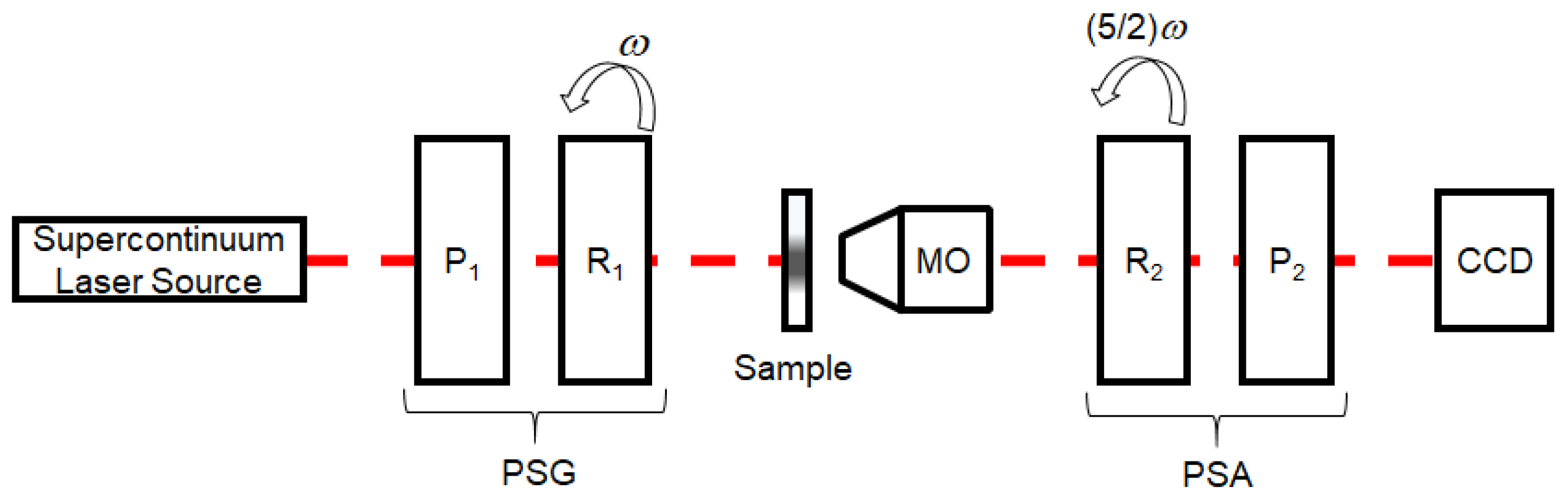
Figure 1 shows the instrument used in the experiment, a dynamic rotating compensator polarimeter whose calibration and use were fully described in previous works [34,35]. It consisted of a Polarization State Generator (PSG) composed of a Polarizer (P1) and a Retarder (R1), a sample holder, a 5× Microscope Objective (MO) with a numerical aperture of 0.15 aligned in the transmission configuration, which allowed studying the sample in the microscopic range, and a Polarizer State Analyzer (PSA), which in turn was composed of another retarder (R2) and an analyzer (P2). The microscope objective was interchangeable so that measurements with different magnifications were possible. Finally, the images were captured with a 12-bit camera. Both retarders rotated synchronously with a speed ratio of 5/2, completing a full Fourier measurement cycle of 200 images of 640 × 640 pixels with which the low noise MM was calculated by means of a Fourier transformation algorithm [36]. Retarder R1 rotated in angular steps of 2/200 rad. In total, the full process of one measurement required 10 min.
The light source was a supercontinuum laser (FemtoPower 1060 made by Fianium), which allowed performing measurements in the visible spectrum, from 480–680 nm. The wavelength selection was performed by a calibrated diffraction grating and a diaphragm. For the results shown here, the wavelength was centered at = 634 nm with a FWHM = 3 nm, a spectral width high enough to lose coherency and avoid a speckle pattern.
3.2. Samples Description
The samples used in this experiment corresponded to two myelomonocytic leukemia cell lines, THP1 and U937, and a colorectal adenocarcinoma cell line, HT29, all provided by ATCC (American Type Culture Collection). The number of deposited cells was chosen so that a uniform layer of cells was achieved, without gaps or piles of cells. Cells were treated with 20 g/mL of cisplatin, a commonly-used chemotherapy drug that induces cell death. Cell viability at 4 different time points was determined by both the trypan blue exclusion test [37], which discriminates between live and dead cells, and the Alamar Blue assay [38], an indicator of cell metabolic activity. Both assays gave us robust information about the cellular health following the cytotoxic treatment. Then, the polarimetric measurements were carried out at 24, 48, and 72 h after the drug was applied. For each period of time, cells were centrifuged, resuspended in Phosphate-Buffered Saline (PBS), and placed on a microscope slide by applying a cytospin technique [39] at 500 r.p.m for 5 min (a high-speed centrifugation to remove the liquid and concentrate the cells on a slide in a layer of 6 mm in diameter). In order to maintain a humid environment for cells (so that they were stable over time) and to prevent the formation of salt crystals, cells were covered with 60 L of 0.3% agarose, which also kept the cells still during the measurement process.
An important issue concerning the samples was the reduction of the surface covered by cells during the treatment. Because of this, as the treatment progressed, the polarimetric signal came from both the background (agarose) and the cells, according to the filling factor reached by the cells in the image, . In order to account for this effect, we introduced a corrected signal that verified:
where is the total value of the polarimetric signal obtained in the measured image and is the polarimetric signal coming from the “empty” background (agarose in our case). The filling factor was calculated for each image by converting them to 8 bit. Then, the image was binarized selecting a threshold that converted pixels occupied by a cell to black and pixels from the background to white (this was done with the free software ImageJ, and the result was double checked by eye inspection).
4. Results and Discussion
4.1. Calibration
A calibration cycle was performed on a target-free configuration in order to characterize the performance of the measuring instrument. During this process, some of the working parameters of the polarimeter were obtained.
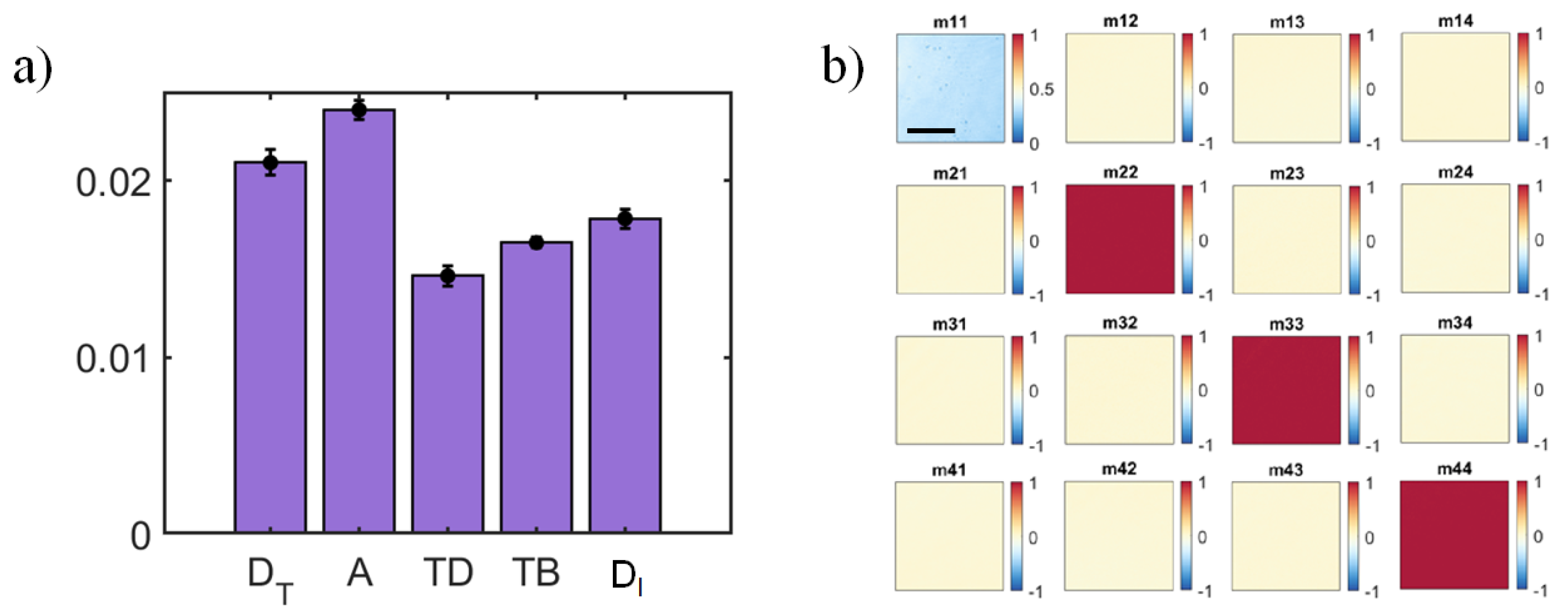
Figure 2b shows a calibration Mueller matrix which had to be ideally the 4 × 4 identity matrix, that is the Mueller matrix of the vacuum, except for the element m, which represents the intensity distribution of the illumination. From a calibration measurement, we can obtain the mean values of the polarimetric magnitudes employed throughout this work (Figure 2a). They can be used as a reference for sensitivity in the actual measurement of samples. Ideally, these values are supposed to be zero.
The processed image was 640 × 640 pixels. After the decomposition of the matrix, we show the images that illustrate the distribution of the main polarimetric magnitudes. However, only the mean values of those images were used for quantitative purposes, with a relative error that was always over the lower limit given by the calibration ( was the largest deviation from 0 or 1 of all 15 elements of the normalized MM).
4.2. Measurement of the Mueller Matrices of Cells
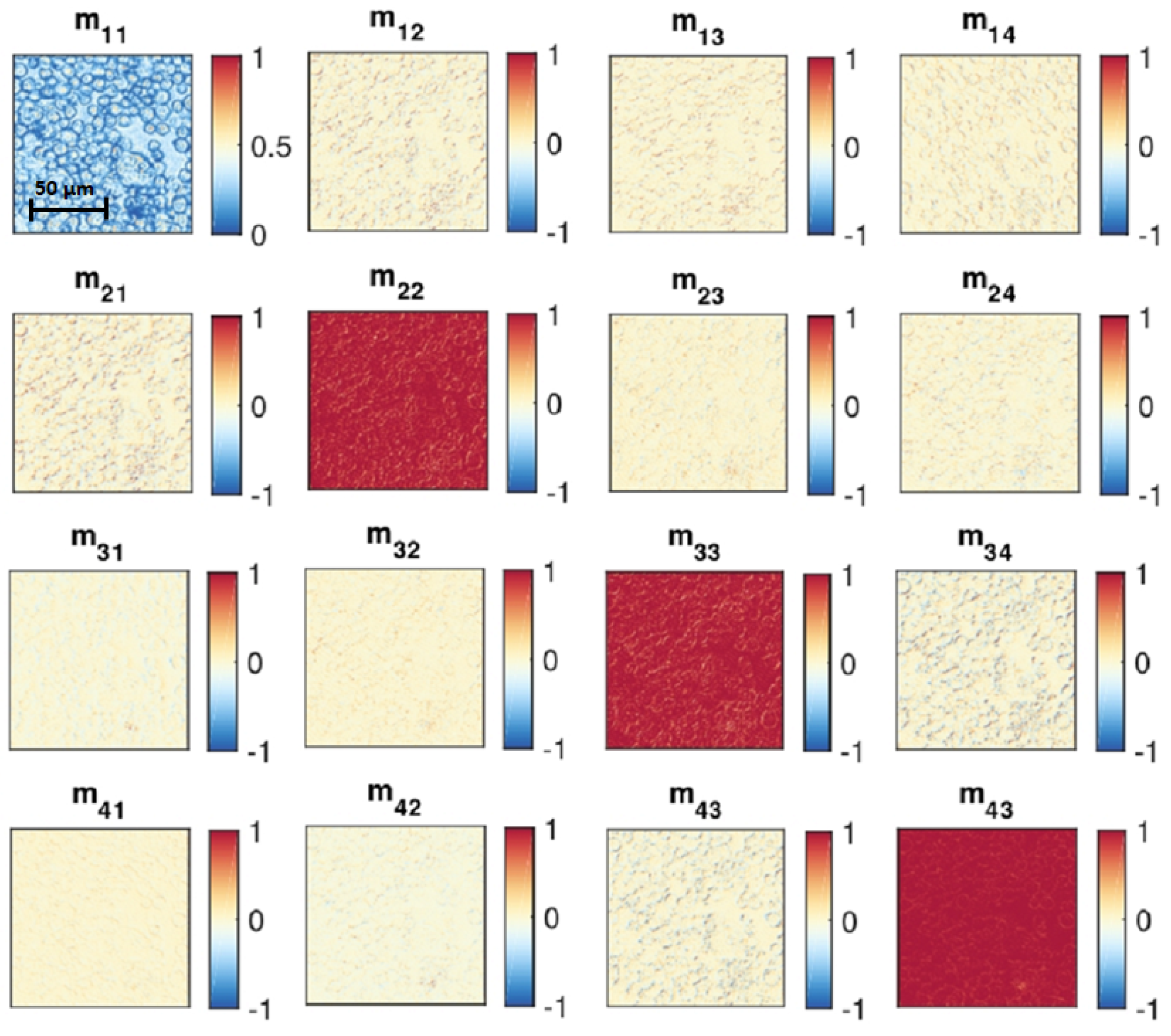
We performed a polarimetric study on three different cell lines, measuring the Mueller matrix and decomposing it in order to calculate different polarimetric magnitudes. As an example, Figure 3 shows the MM for a sample of HT29 cells on a microscope slide. Cells had an approximate diameter of 10–15 m. The element of the Mueller matrix represents the intensity (a regular image of the object plane) where the locations of individual cells and their membranes are clearly visible.
At first glance, the Mueller matrices of cells resembled a unitary matrix, showing that the optical activity of this sample under transmission observation and ordinary illumination conditions was very small. The different decompositions showed that samples hardly introduced any significant amount of diattenuation, retardance, optical rotation, or depolarization. However, some signal can be found apparently in the boundaries of the cells. Among all the polarimetric magnitudes introduced in the analysis methods previously mentioned, we focused our attention on diattenuation, since it seemed to offer the most significant results. Other magnitudes such as A, TD, and TB were also addressed.
4.3. Cell State Assessment: Quantifying Cell Death
U937 leukemia cells were used to perform the polarimetric study related to the effect of a chemotherapy treatment. Cells were treated with the cytotoxic drug cisplatin. Viability tests were performed at 24, 48, and 72 h after treatment. In addition, polarimetric measurements of samples deposited on a microscope slide were carried out. Control (non-treated) and treated cells were compared.
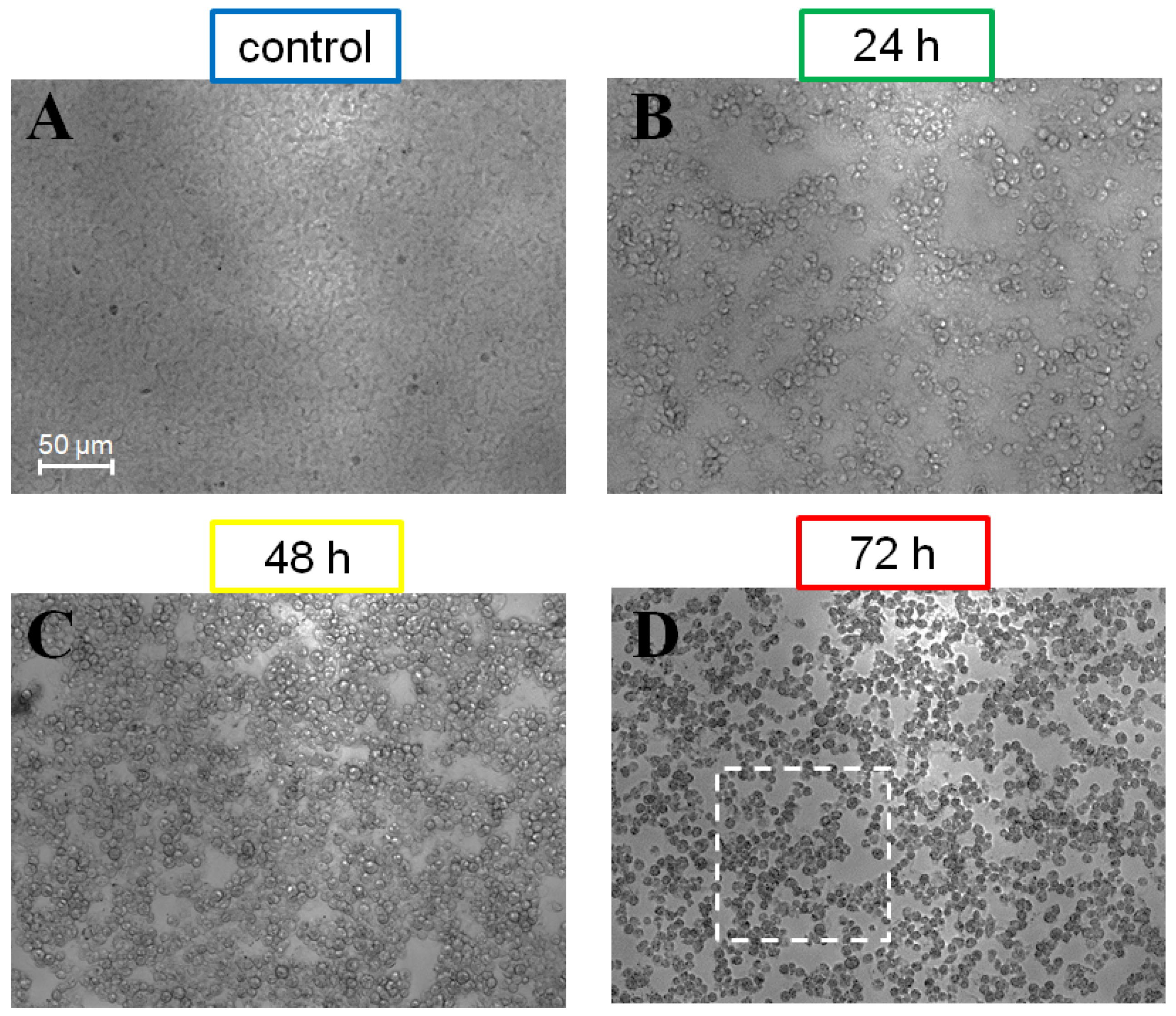
Ordinary microscopic images (Figure 4) showed the differences between untreated (A) and the cisplatin-treated cells at 24 (B), 48 (C), and 72 (D) hours. Cisplatin-treated U937 cells were less confluent, showed cell shrinkage, and became pyknotic (with cytoplasmic and nuclear condensation) at longer times, mostly for 72 h (Figure 4D). These morphological features are associated with apoptotic cell death [40], and it is well established that cisplatin induces apoptosis in a number of cancer cells, including U937 cells [41].
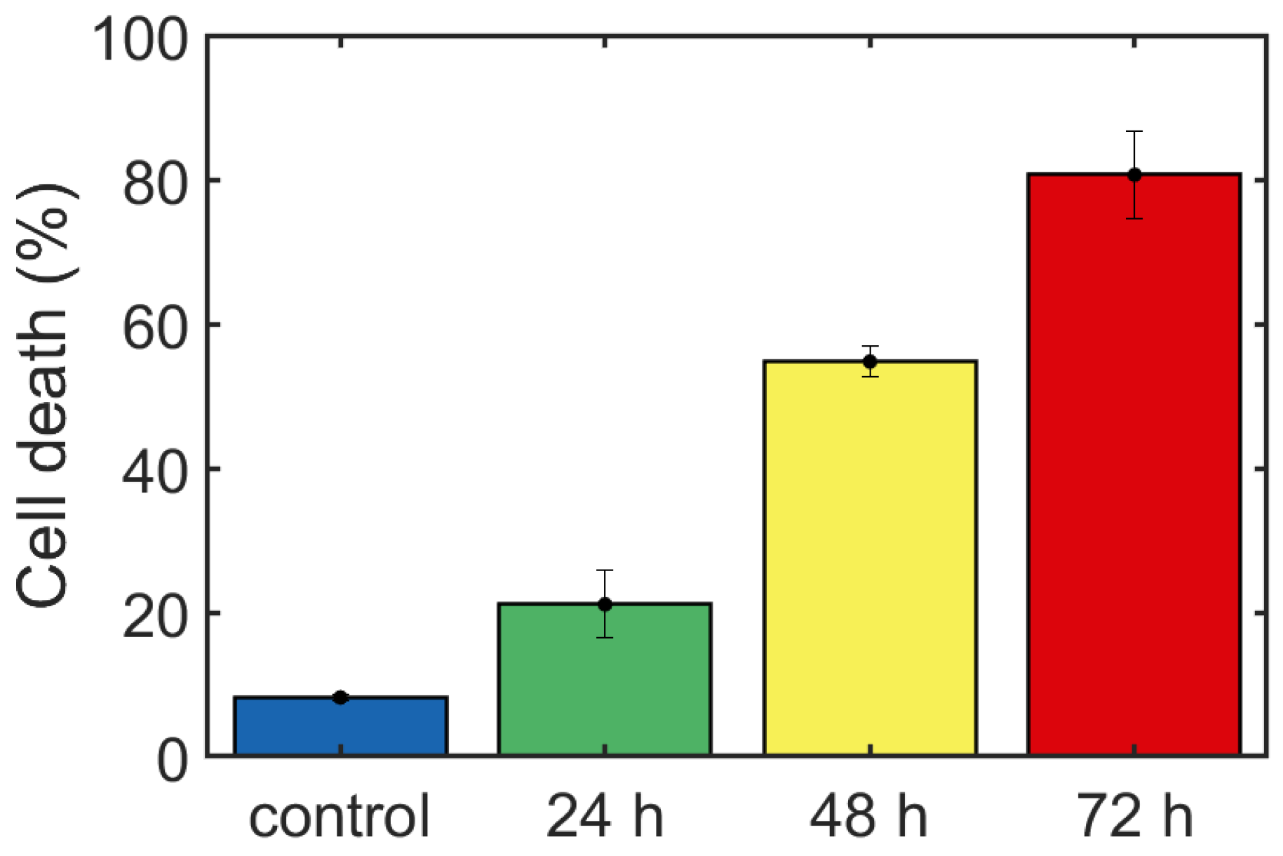
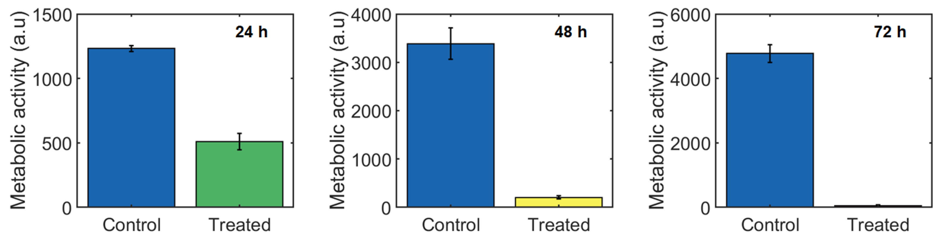
We performed the trypan blue assay to evaluate cell viability at different time points of treatment (Figure 5). Cell mortality gradually increased over time, reaching about 80% cell death by 72 h. This result was confirmed by showing that cisplatin reduced the metabolic activity of U937 cells from 2.4-fold at 24 h to 100-fold at 72 h, corresponding to cells undergoing cell death (Figure 6).
After that, five images (640 × 640 pixels) of the Mueller matrix were measured in five different regions of each of the four samples. The five different regions were randomly selected in the area covered by the cells (circle of 6 mm in diameter). The dashed white square in Figure 4D) represents the size of the image taken with the polarimeter (180 × 180 m approximately). Some polarimetric magnitudes were obtained by applying different decomposition methods, and finally, in order to analyze the results, the mean values of each magnitudes were calculated. Figure 7a shows the mean value of the five images of diattenuation for each sample. A slight, but significant increase was observed at 24 h (p-values obtained with both tests were 0.016), when cell death was about 25%. Great differences were observed by 48 h of treatment, when the cell death was above 50%. As was explained in Section 3, we found that the results were highly dependent on cell confluence, this is the filling factor of the image. In Figure 7, both the raw results and those corrected according to Equation (12) are represented. Then, we used two statistical non-parametric tests to check if it was possible to tell apart one measurement set from another. We applied the Wilcoxon rank test and the Kruskal–Wallis test to our set of data and obtained the corresponding p-values (Table 1).
Statistical analysis tells us that there was a significant difference between the population of untreated (control) and treated cells (p-values < 0.05). This confirms that we were able to detect even low percentages of cell death. At longer times, the correlation between cell death and diattenuation became stronger with p-values smaller than 0.01.
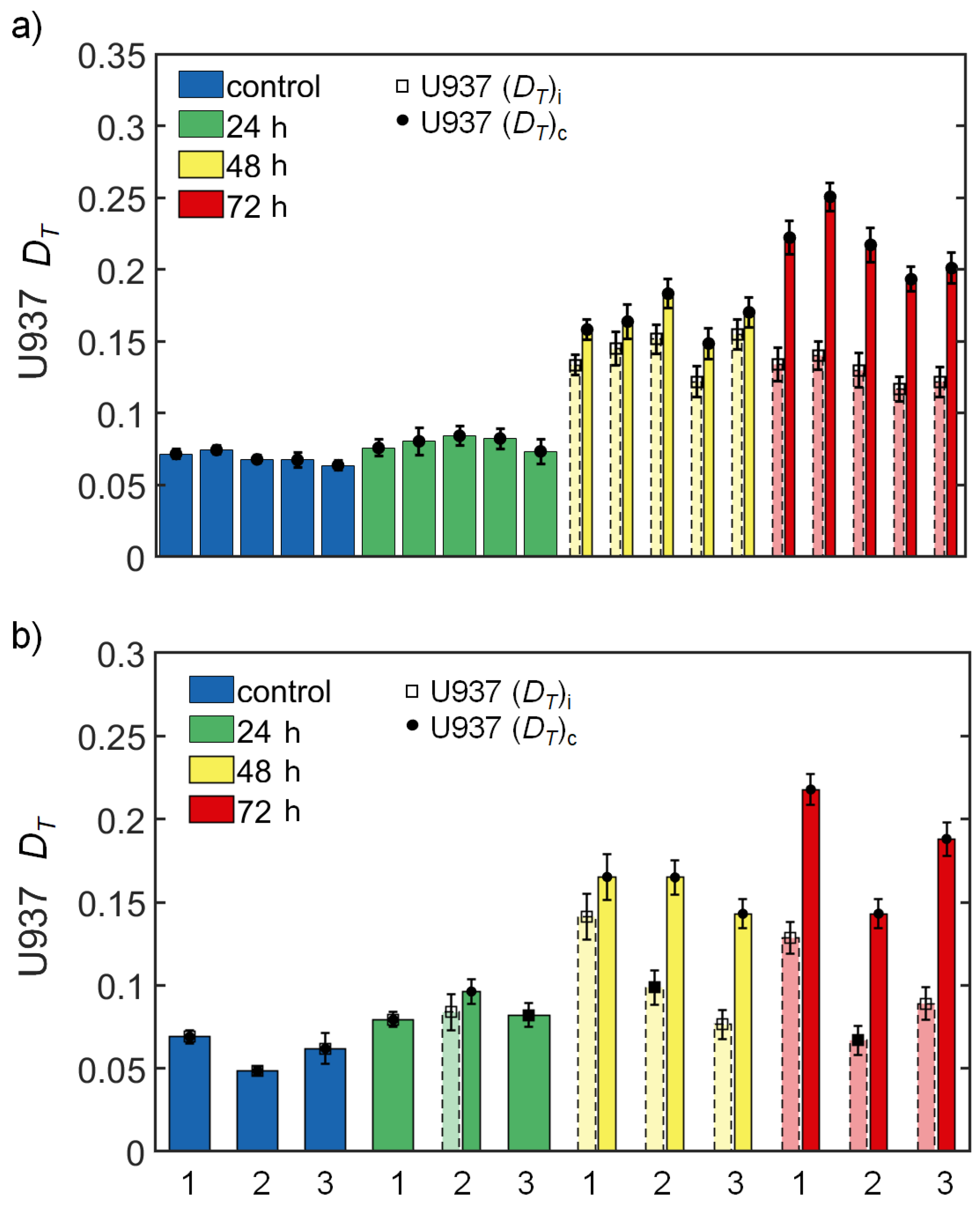
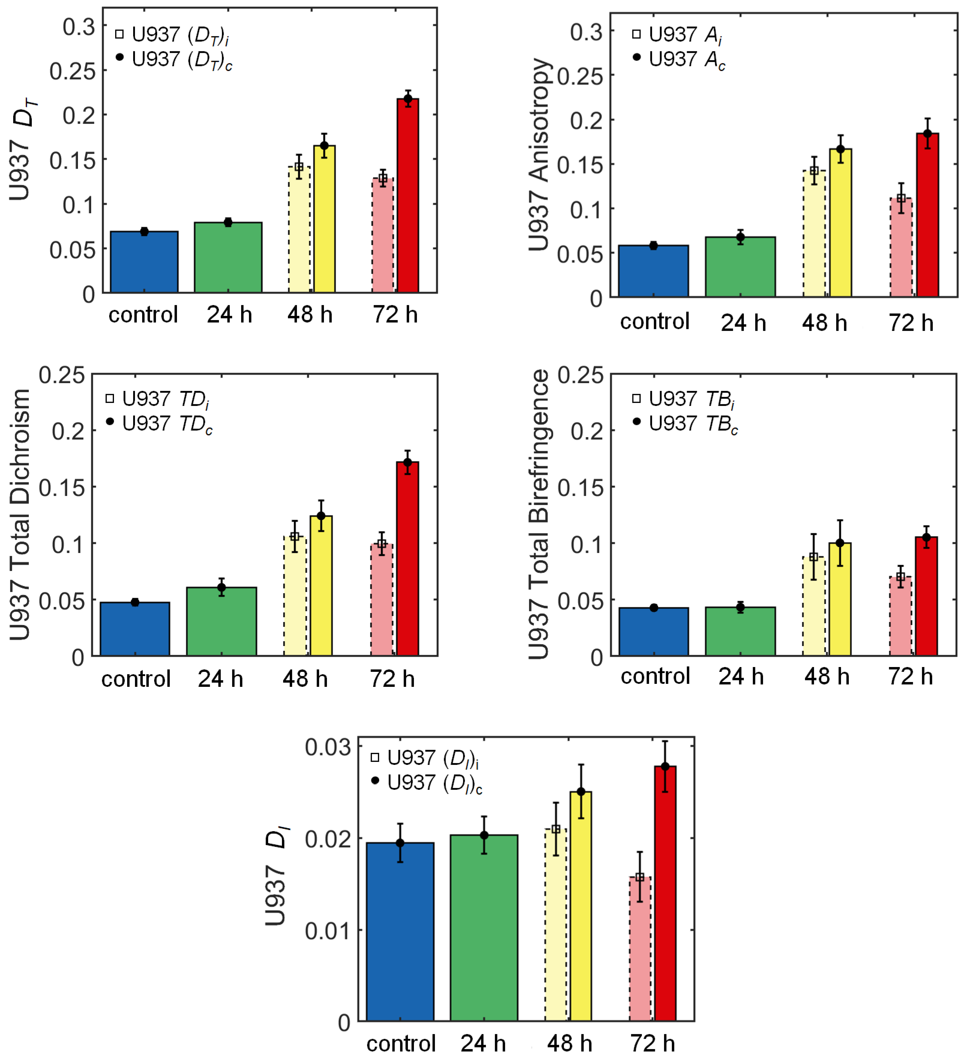
Other polarimetric magnitudes obtained from different decomposition methods showed a similar variation over time. We considered that values of the depolarization index corresponding to the samples were too small and close to the values obtained in the calibration (Figure 2a) to be significant. Figure 8 shows the evolution of the element (intensity image) and five polarimetric magnitudes (total diattenuation, anisotropy, total dichroism, total birefringence, and depolarization index) over time before and after applying the filling factor correction. Bars represent the mean values of all the pixels of the five images taken in each sample. The intensity image () was not useful for extracting conclusions because was a non-normalized parameter, and it depended on the illumination and on the integration time of the camera. However, all five magnitudes seemed to be sensitive to the cell death and presented a similar trend over time. We decided to focus our study on diattenuation because it presented the lowest standard deviation. Once focused on diattenuation, we performed our experiment in triplicate. Results are shown in Figure 7b, where the mean values of diattenuation are presented for each experiment and for each time point.
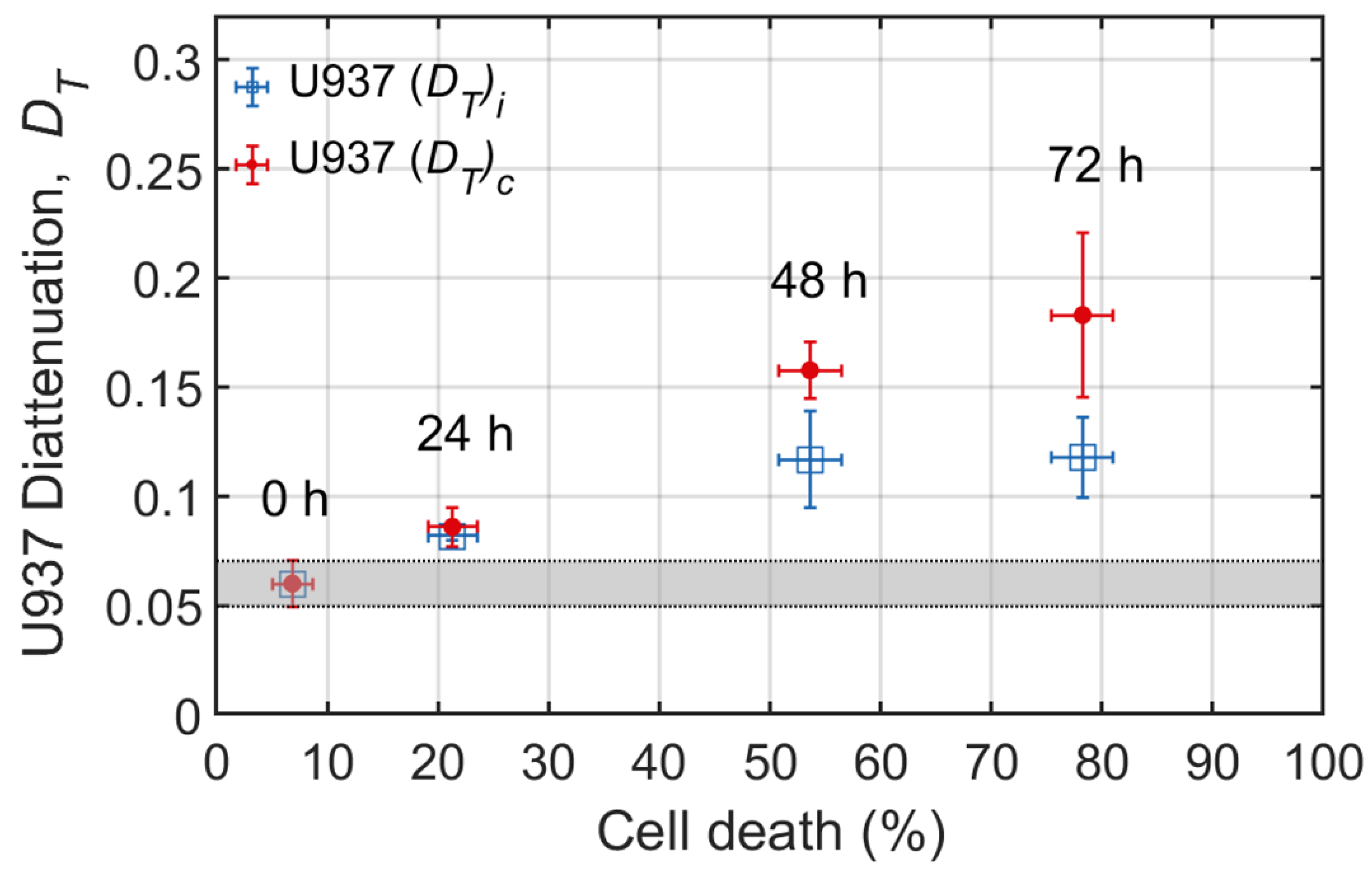
In Figure 9, we show the correlation between the mean values of diattenuation and the mean value of the percentage of dead cells obtained from the triplicate experiment with U937 cells. Both diattenuation and cell death increased over time. At 24 h, there was a slight increase in diattenuation that became very significant at 48 h of treatment. If data were not corrected by the filling factor, by 72 h, the diattenuation slightly decreased with respect to the previous time point, likely due to the loss of cell confluency, as shown in Figure 4D, which would decrease the mean value of the parameter measured. After correction we see that the diattenuation increased with the cell death.
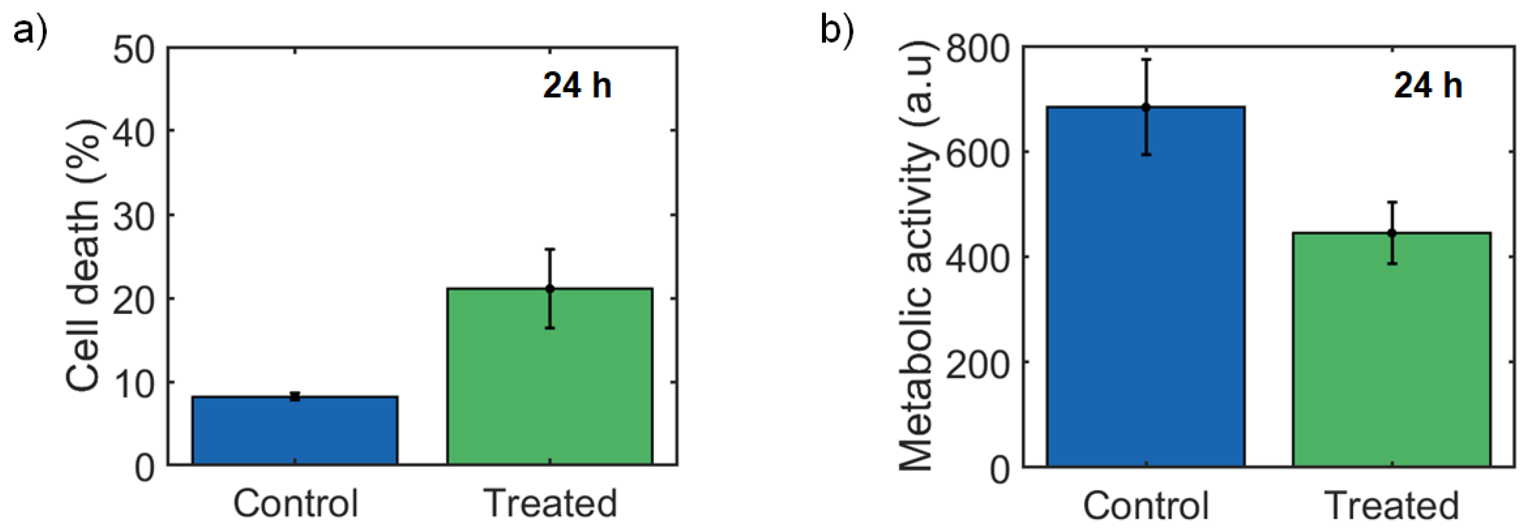
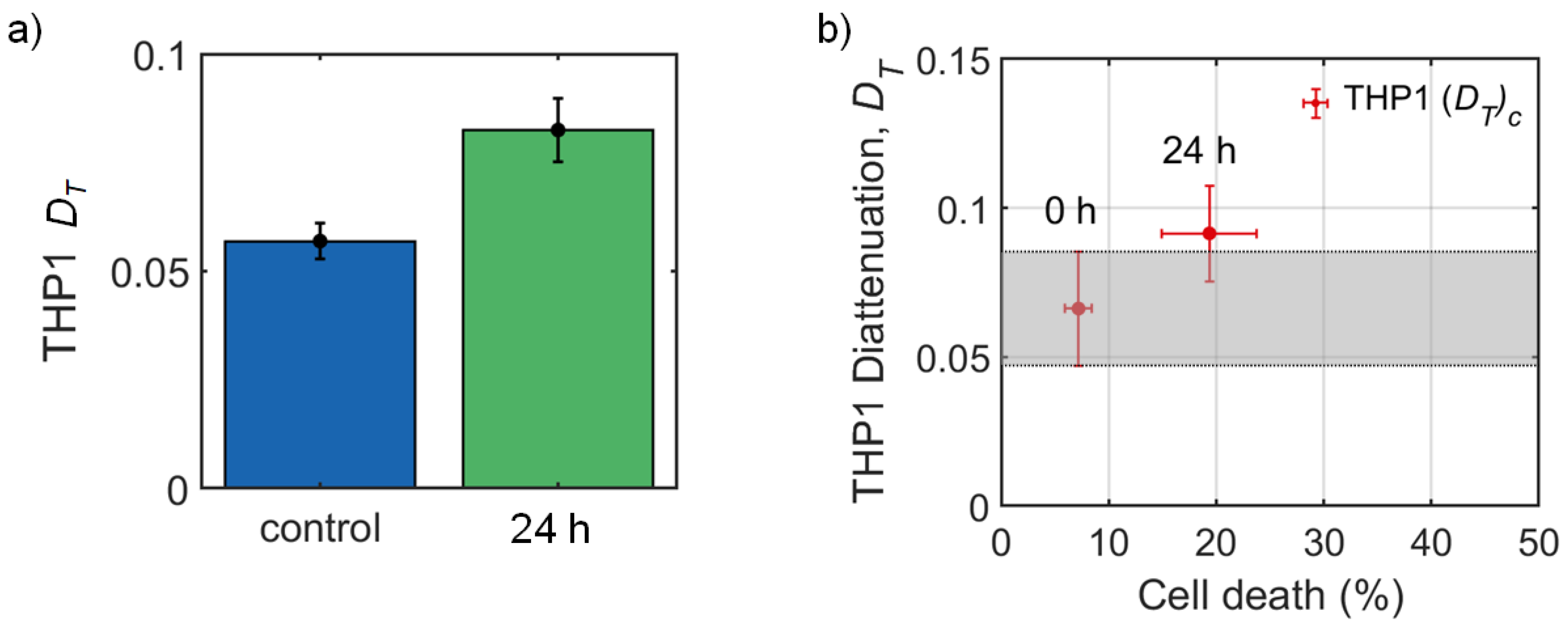
A similar result was obtained when another leukemia cell line, THP1, was treated with cisplatin. By 24 h of treatment, there was over a two-fold increase of cell death by trypan blue (Figure 10a), which was confirmed by a reduction of metabolic activity (Figure 10b). Consistent with our previous data, the diattenuation significantly increased (p = 0.008 with the Wilcoxon rank test) after treatment with cisplatin for 24 h (Figure 11a)). Results for the triplicate experiment are shown in Figure 11b). The trypan blue test showed a high dispersion in these results, and the diattenuation increase was accordingly noisy. Overall, the evolution was similar to that observed in Figure 7.
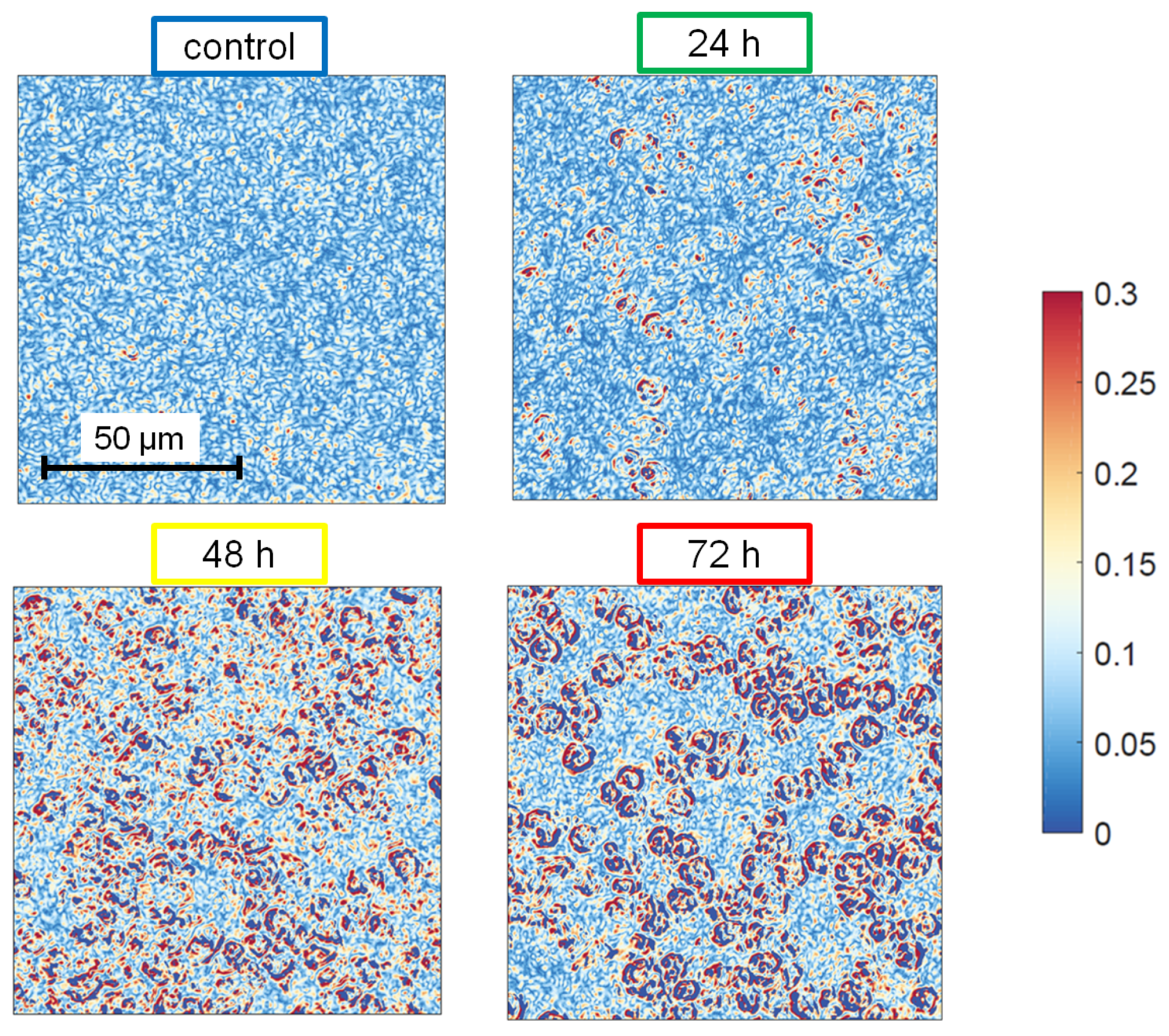
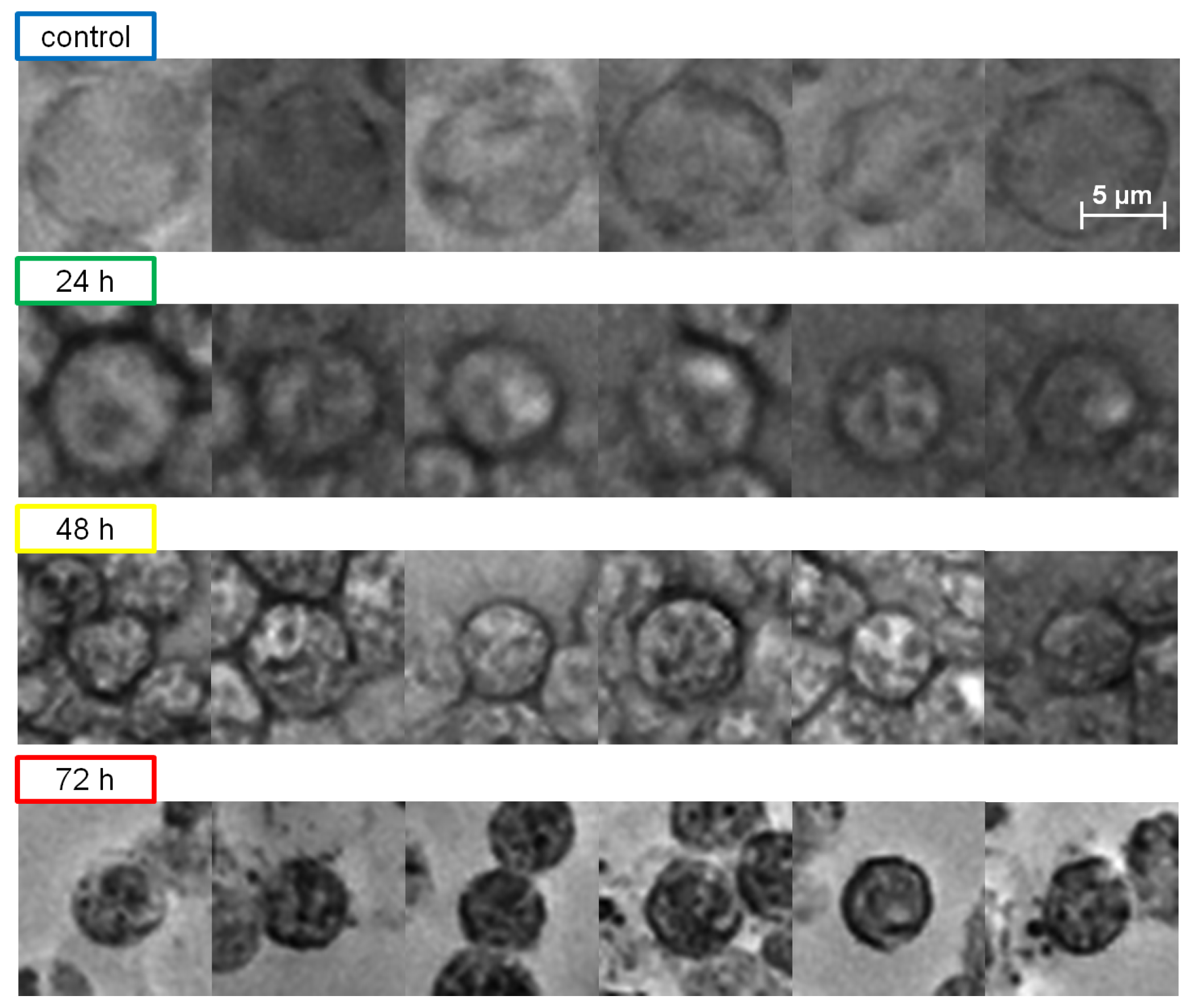
Paying attention to the spatial distribution of in the image (see Figure 12), it seems that the diattenuation enhancement associated with cell death and observed in both U937 and THP1 cells was most likely the consequence of changes in the plasma membrane. As can be seen in Figure 12, where four images of the total diattenuation parameter are shown for different treatment times, the increase of the signal was observed mainly at the cell boundary and clearly outlined its contour. This is in agreement with the fact that plasma membranes suffer major changes during the apoptosis process, including loss of phospholipid asymmetry. This phospholipid redistribution between inner and outer leaflets of the membrane generates interfacial forces able to modify the structure of transmembrane proteins [42], which could be detected by using circular dichroism, a well-known technique that has been employed for studying the structure, dynamics, and interactions of proteins [43] in the UV domain. Another effect that modifies the value of the diattenuation during cell death results from alterations in membrane tension due to modification of membrane-associated molecules and the intracellular and extracellular mechanical stimuli that change the membrane curvature [44]. The morphological changes associated with this effect are in agreement with the appearance offered by U937 cells in the different treatment time points, as shown in Figure 13. Thus, we suggest that the increase of the diattenuation signal could be related to changes in transmembrane protein structure and membrane geometry as cells undergo apoptosis.
5. Conclusions
We measured the image Mueller matrix in the transmission configuration of biological samples corresponding to the colorectal adenocarcinoma HT29 cell line and leukemia cell lines U937 and THP1. On such matrices, we performed polar decomposition, Mueller matrix transformation, and differential decomposition in order to reach several polarimetric magnitudes that could give us more insight into the role played by the cell, or by some cell components, in changing the polarization of the light that goes through it either in the living state or when it undergoes apoptosis.
As expected, since living cells are mainly transparent with an index of refraction close to water [17], the resulting matrix was quite close to unity. The main deviations from the trivial values after MM analysis were found in the diattenuation (after MMPD), anisotropy, (after MMT), total dichroism, and total birefringence (after MMDD).
In this research, a study of cell death was performed, combining a traditional method with others based on the measurement and analysis of the above-mentioned polarimetric magnitudes. U937 and THP1 leukemia cells were treated with a chemotherapy drug in order to induce cell death. Observation under the microscope showed evidence of cell degradation, but its quantification was not a straightforward process. When performing the polarimetric analysis on U937 cells, a strong correlation between diattenuation and cell death was clearly observed, even at early times after treatment. In addition, we suggest that, since the diattenuation signal was located at the boundaries of cells, the increasing of diattenuation could be related to changes in the plasma membrane geometry and in its protein structure as cells undergo apoptosis. Similar results were obtained for the THP1 cell line and other polarimetric magnitudes mentioned above.
We conclude that diattenuation could be an objective parameter to detect cell death and useful for assessing in vitro killing efficacy of drugs under development and the follow-up of leukemia patients undergoing therapy with cytotoxic agents. Although the type of cell death detected is likely to be apoptotic because cisplatin treatment induces apoptosis, further studies will reveal whether diattenuation is able to discriminate between the different types of cell death. Moreover, since this method could be implemented in a microscope, although further work is necessary, it could result in an objective (i.e., independent of the observer) polarimetric method of analysis, complementary to the traditional techniques used for cell death quantification.
Author Contributions
Conceptualization, all authors; methodology, A.F.-P. and O.G.-S.; software, A.F.-P.; validation, all authors; formal analysis, A.F.-P.; investigation, A.F.-P. and O.G.-S.; resources, J.L.F.-L., F.M., and J.M.S.; data curation, A.F.-P. and O.G.-S.; writing, original draft preparation, A.F.-P.; writing, review and editing, J.M.S., F.M., J.L.F.-L., and A.F.-P.; visualization, A.F.-P.; supervision, J.M.S., J.L.F.-L., and F.M.; project administration, J.L.F.L. and J.M.S.; funding acquisition, J.L.F.-L., F.M., and J.M.S.
Funding
This work has been supported by a grant from Instituto de Investigacion Valdecilla (IDIVAL) APG/03 to J.L.F.-L. and by SODERCAN (Sociedad para el Desarrollo de Cantabria) and Research Vicerrectorate of the University of Cantabria through Project 14JU2864661. A.F.-P. acknowledges the University of Cantabria for her FPUgrant.
Conflicts of Interest
The authors declare no conflict of interest. The funders had no role in the design of the study; in the collection, analyzes, or interpretation of the data; in the writing of the manuscript; nor in the decision to publish the results.
Abbreviations
The following abbreviations are used in this manuscript:
| MM | Mueller Matrix |
| S | Stokes vector |
| MMPD | Mueller Matrix Polar Decomposition |
| MMT | Mueller Matrix Transformation |
| MMDD | Mueller Matrix Differential Decomposition |
| PSG | Polarization State Generator |
| PSA | Polarization State Analyzer |
| Wavelength | |
| P | Polarizer |
| R | Retarder |
| MO | Microscope Objective |
| Total diattenuation | |
| A | Anisotropy |
| Depolarization index | |
| Total Dichroism | |
| Total Birefringence | |
| Linear Dichroism | |
| Circular Dichroism | |
| Linear Birefringence | |
| Circular Birefringence | |
| Filling factor |
References
- Chipman, R.A. Polarimetry. In Handbook of Optics; OSA: Washington, DC, USA, 1995; pp. 22.21–22.35. [Google Scholar]
- Hough, J. Polarimetry: A powerful diagnostic tool in astronomy. Astron. Geophys. 2006, 47, 31–35. [Google Scholar] [CrossRef]
- Tyo, J.S.; Goldstein, D.L.; Chenault, D.B.; Shaw, A.J. Review of passive imaging polarimetry for remote sensing applications. Appl. Opt. 2006, 45, 5453–5469. [Google Scholar] [CrossRef] [PubMed] [Green Version]
- He, H.; Chang, J.; He, C.; Ma, H. Transformation of full 4 × 4 Mueller matrices: A quantitative technique for biomedical diagnosis. In Proceedings of the SPIE BiOS 2016, San Francisco, CA, USA, 13 February 2016; p. 97070K. [Google Scholar] [CrossRef]
- Ghosh, N. Tissue polarimetry: Concepts, challenges, applications, and outlook. J. Biomed. Opt. 2011, 16, 110801. [Google Scholar] [CrossRef]
- Ahmad, I.; Ahmad, M.; Khan, K.; Ashraf, S.; Ahmad, S.; Ikram, M. Ex vivo characterization of normal and adenocarcinoma colon samples by Mueller matrix polarimetry. J. Biomed. Opt. 2015, 20, 056012. [Google Scholar] [CrossRef] [PubMed]
- Pierangelo, A.; Benali, A.; Antonelli, M.R.; Novikova, T.; Validire, P.; Gayet, B.; De Martino, A. Ex-vivo characterization of human colon cancer by Mueller polarimetric imaging. Opt. Express 2011, 19, 1582–1593. [Google Scholar] [CrossRef]
- Pierangelo, A.; Nazac, A.; Benali, A.; Validire, P.; Cohen, H.; Novikova, T.; Ibrahim, B.H.; Manhas, S.; Fallet, C.; Antonelli, M.R.; et al. Polarimetric imaging of uterine cervix: A case study. Opt. Express 2013, 21, 14120–14130. [Google Scholar] [CrossRef]
- Vizet, J.; Rehbinder, J.; Deby, S.; Roussel, S.; Nazac, A.; Soufan, R.; Genestie, C.; Haie-Meder, C.; Fernandez, H.; Moreau, F.; et al. In vivo imaging of uterine cervix with a Mueller polarimetric colposcope. Sci. Rep. 2017, 7, 2471. [Google Scholar] [CrossRef]
- He, H.; Zeng, N.; Sun, M.; Guo, Y.; Wu, J.; Liu, S. Mueller matrix polarimetry for differentiating characteristic features of cancerous tissues characteristic features of cancerous tissues. J. Biomed. Opt. 2014, 19, 070504. [Google Scholar] [CrossRef]
- Ahmad, I.; Ahmad, M.; Khan, K.; Ikram, M. Polarimetry based partial least square classification of ex vivo healthy and basal cell carcinoma human skin tissues. Photodiagn. Photodyn. Therapy 2016, 14, 134–141. [Google Scholar] [CrossRef]
- Gurjar, R.S.; Backman, V.; Perelman, L.T.; Georgakoudi, I.; Badizadegan, K.; Itzkan, I.; Dasari, R.R.; Feld, M.S. Imaging human epithelial properties with polarized light-scattering spectroscopy. Nat. Med. 2001, 7, 1245–1248. [Google Scholar] [CrossRef]
- Firdous, S.; Atif, M.; Nawaz, M. Study of Blood Malignancy in Vitro for the Diagnosis and Treatment of Blood Diseases Using Polarimetery and Microscopy. Lasers Eng. 2010, 19, 291–305. [Google Scholar]
- Menzel, M.; Axer, M.; Amunts, K.; Raedt, H.D.; Michielsen, K. Diattenuation Imaging reveals different brain tissue properties. Sci. Rep. 2019, 9, 1939. [Google Scholar] [CrossRef]
- Ceolato, R.; Riviere, N.; Jorand, R.; Ducommun, B.; Lorenzo, C. Light-scattering by aggregates of tumor cells: Spectral, polarimetric, and angular measurements. J. Quant. Spectrosc. Radiat. Transf. 2014, 146, 207–213. [Google Scholar] [CrossRef]
- Ding, H.; Lu, J.Q.; Brock, R.S.; McConnell, T.J.; Ojeda, J.F.; Jacobs, K.M.; Hu, X.H. Angle-resolved Mueller matrix study of light scattering by B-cells at three wavelengths of 442, 633, and 850 nm. J. Biomed. Opt. 2013, 12, 34032. [Google Scholar] [CrossRef]
- Choi, W.J.; Jeon, D.I.; Ahn, S.G.; Yoon, J.H.; Kim, S.; Lee, B.H. Full-field optical coherence microscopy for identifying live cancer cells by quantitative measurement of refractive index distribution. Opt. Express 2010, 18, 23285. [Google Scholar] [CrossRef]
- Liu, P.Y.; Chin, L.K.; Ser, W.; Chen, H.F.; Hsieh, C.M.; Lee, C.H.; Sung, K.B.; Ayi, T.C.; Yap, P.H.; Liedberg, B.; et al. Cell refractive index for cell biology and disease diagnosis: Past, present and future. Lab Chip 2016, 16, 634–644. [Google Scholar] [CrossRef]
- Gil, J.J.; Ossikovski, R. Polarized Light and the Mueller Matrix Approach, 2016th ed.; Taylor & Francis: Abingdon, UK, 2016. [Google Scholar]
- Lu, S.Y.; Chipman, R.A. Interpretation of Mueller matrices based on polar decomposition. J. Opt. Soc. Am. A 1996, 13, 1106–1113. [Google Scholar] [CrossRef]
- He, H.; Zeng, N.; Du, E.; Guo, Y.; Li, D.; Liao, R.; Ma, H. A possible quantitative Mueller matrix transformation technique for anisotropic scattering media. Photonics Lasers Med. 2013, 2, 129–137. [Google Scholar] [CrossRef]
- Azzam, R.M.A. Propagation of partially polarized light through anisotropic media with or without depolarization: A differential 4 × 4 matrix calculus. J. Opt. Soc. Am. 1978, 68, 1756–1767. [Google Scholar] [CrossRef]
- Shrestha, S.; Deshpande, A.; Farrahi, T.; Cambria, T.; Quang, T.; Majeski, J.; Na, Y.; Zervakis, M.; Livanos, G.; Giakos, G.C. Label-free discrimination of lung cancer cells through mueller matrix decomposition of diffuse reflectance imaging. Biomed. Signal Process. Control 2017, 40, 505–518. [Google Scholar] [CrossRef]
- Jiang, W.; Lu, J.Q.; Yang, L.V.; Sa, Y.; Feng, Y.; Ding, J.; Hu, X.H. Comparison study of distinguishing cancerous and normal prostate epithelial cells by confocal and polarization diffraction imaging. J. Biomed. Opt. 2015, 21, 071102. [Google Scholar] [CrossRef] [PubMed]
- Liu, Z.; Liao, R.; Wan, J.; Ma, H.; Leung, P.T.; Yan, M.; Wai, T.C.; Gu, J. Polarization staining and high-throughput detection of marine microalgae using single cell average Mueller matrices. Optik 2019, 180, 84–90. [Google Scholar] [CrossRef]
- Li, X.; Liao, R.; Zhou, J.; Leung, P.T.; Yan, M.; Ma, H. Classification of morphologically similar algae and cyanobacteria using Mueller matrix imaging and convolutional neural networks. Appl. Opt. 2017, 56, 6520–6530. [Google Scholar] [CrossRef] [PubMed]
- Badieyan, S.; Dilmaghani-Marand, A.; Hajipour, M.J.; Ameri, A.; Razzaghi, M.R.; Rafii-Tabar, H.; Mahmoudi, M.; Sasanpour, P. Detection and Discrimination of Bacterial Colonies with Mueller Matrix Imaging. Sci. Rep. 2018, 8, 10815. [Google Scholar] [CrossRef] [PubMed]
- Gil, J.J. On optimal filtering of measured Mueller matrices. Appl. Opt. 2016, 55, 5449–5455. [Google Scholar] [CrossRef] [PubMed]
- Ossikovski, R. Differential matrix formalism for depolarizing anisotropic media. Opt. Lett. 2011, 36, 2330–2332. [Google Scholar] [CrossRef] [PubMed]
- Rwin, H.A.; Alván, A.M.E.; Agnusson, R.M.; Ndersson, A.A.; Andin, J.L.; Ärrendahl, K.J.; Aurel, E.G.A.; Ssikovski, R.O.; Arwin, H.; Mendoza-Galván, A.; et al. Structural circular birefringence and dichroism quantified by differential decomposition of spectroscopic transmission Mueller matrices from Cetonia aurata. Opt. Lett. 2016, 41, 3293–3296. [Google Scholar] [CrossRef] [Green Version]
- Occidentale, B.; Laser, O.; Gorgeu, A.L.; Cedex, B.; Society, O.; Ocis, A. Scanning Mueller polarimetric microscopy. Opt. Lett. 2016, 41, 4336–4339. [Google Scholar]
- Zhou, J.; Wang, Y. Modulus design multiwavelength polarization microscope for transmission Mueller matrix imaging Modulus design multiwavelength polarization microscope for transmission Mueller matrix imaging. J. Biomed. Opt. 2018, 23, 016007. [Google Scholar] [CrossRef]
- Arteaga, O.; Baldrís, M.; Antó, J.; Canillas, A.; Pascual, E.; Bertran, E. Mueller matrix microscope with a dual continuous rotating compensator setup and digital demodulation. Appl. Opt. 2014, 53, 2236–2245. [Google Scholar] [CrossRef] [Green Version]
- Sanz, J.M.; Extremiana, C.; Saiz, J.M. Comprehensive polarimetric analysis of Spectralon white reflectance standard in a wide visible range. Appl. Opt. 2013, 52, 6051. [Google Scholar] [CrossRef] [PubMed]
- Carmagnola, F.; Sanz, J.M.; Saiz, J.M. Development of a Mueller matrix imaging system for detecting objects embedded in turbid media. J. Quant. Spectrosc. Radiat. Transf. 2014, 146, 199–206. [Google Scholar] [CrossRef]
- Azzam, R.M. Photopolarimetric measurement of the Mueller matrix by Fourier analysis of a single detected signal. Opt. Lett. 1978, 2, 148. [Google Scholar] [CrossRef] [PubMed]
- Strober, W. Trypan Blue Exclusion Test of Cell Viability. Curr. Protoc. Immunol. 2015, 111. [Google Scholar] [CrossRef] [PubMed]
- Rampersad, S.N. Multiple applications of alamar blue as an indicator of metabolic function and cellular health in cell viability bioassays. Sensors 2012, 12, 12347–12360. [Google Scholar] [CrossRef] [PubMed]
- Koh, C.M. Preparation of Cells for Microscopy Using Cytospin, 1st ed.; Elsevier Inc.: Amsterdam, The Netherlands, 2013; Volume 533, pp. 235–240. [Google Scholar]
- Taatjes, D.J.; Sobel, B.E.; Budd, R.C. Morphological and cytochemical determination of cell death by apoptosis. Histochem. Cell Biol. 2008, 129, 33–43. [Google Scholar] [CrossRef] [PubMed]
- Shrivastava, P.; Sodhi, A.; Ranjan, P. Anticancer drug-induced apoptosis in human monocytic leukemic cell line U937 requires activation of endonuclease(s). Anti-Cancer Drugs 2000, 11, 39–48. [Google Scholar] [CrossRef] [PubMed]
- Frolov, V.A.; Shnyrova, A.V.; Zimmerberg, J. Lipid Polymorphisms and Membrane Shape. Cold Spring Harb. Perspect. Biol. 2011, 3, a004747. [Google Scholar] [CrossRef]
- Miles, A.J.; Wallace, B.A. Circular dichroism spectroscopy of membrane proteins. Chem. Soc. Rev. 2016, 45, 4859–4872. [Google Scholar] [CrossRef] [Green Version]
- Rysavy, N.M.; Shimoda, L.M.N.; Dixon, A.M.; Speck, M.; Stokes, A.J.; Turner, H.; Umemoto, E.Y. Beyond apoptosis: The mechanism and function of phosphatidylserine asymmetry in the membrane of activating mast cells. BioArchitecture 2014, 4, 127–137. [Google Scholar]
Figure 1.
Schematics of the imaging polarimeter. The light source is a supercontinuum laser; P1 and P2 are Polarizers; R1 and R2 are Retarders (quarter waveplate); MO is the Microscope Objective; PSG and PSA stand for Polarization State Generator and Analyzer, respectively.
Figure 1.
Schematics of the imaging polarimeter. The light source is a supercontinuum laser; P1 and P2 are Polarizers; R1 and R2 are Retarders (quarter waveplate); MO is the Microscope Objective; PSG and PSA stand for Polarization State Generator and Analyzer, respectively.

Figure 2.
(a) Diattenuation (), anisotropy (A), total dichroism (), total birefringence (), and depolarization index () obtained from a calibration measurement. The error bar is the standard deviation. (b) Imaging calibration Mueller matrix. The black scale bar represents 50 m.
Figure 2.
(a) Diattenuation (), anisotropy (A), total dichroism (), total birefringence (), and depolarization index () obtained from a calibration measurement. The error bar is the standard deviation. (b) Imaging calibration Mueller matrix. The black scale bar represents 50 m.

Figure 3.
Experimental Mueller matrix image of HT29 cells performed at = 634 nm with a 5× microscope objective.
Figure 3.
Experimental Mueller matrix image of HT29 cells performed at = 634 nm with a 5× microscope objective.

Figure 4.
U937 sample images taken by phase contrast microscopy. (A) Control sample (non-treated); (B–D) 24, 48, and 72 h after treatment with 20 g/mL of cisplatin. The white dashed square represents the size of the image taken with the polarimeter (640 × 640 pixels.)
Figure 4.
U937 sample images taken by phase contrast microscopy. (A) Control sample (non-treated); (B–D) 24, 48, and 72 h after treatment with 20 g/mL of cisplatin. The white dashed square represents the size of the image taken with the polarimeter (640 × 640 pixels.)

Figure 5.
Cell death of U937 cells over time treated with 20 g/mL of cisplatin evaluated with the trypan blue exclusion test. The error bar is the standard deviation of three measurements.
Figure 5.
Cell death of U937 cells over time treated with 20 g/mL of cisplatin evaluated with the trypan blue exclusion test. The error bar is the standard deviation of three measurements.

Figure 6.
Metabolic activity of U937 cells following a treatment with cisplatin at different time points using the Alamar Blue assay. a.u., arbitrary units. The error bar is the standard deviation of three measurements.
Figure 6.
Metabolic activity of U937 cells following a treatment with cisplatin at different time points using the Alamar Blue assay. a.u., arbitrary units. The error bar is the standard deviation of three measurements.

Figure 7.
Mean diattenuation () of each of the five images taken from the control and cisplatin-treated samples of U937 cells. (a) shows the five measurements taken for each time in the first experiment. (b) shows the mean values at each time for the triplicate experiment (numbered as 1, 2, and 3). Data are shown before (□, dashed bars) and after (•, solid line) applying the the correction given by Equation (12). When the bar is not duplicated, it means that = 1 for the measured image, and no filling correction is required. Error bars represent the standard deviation of the image.

Figure 8.
Mean total diattenuation, anisotropy, total birefringence, total dichroism, and depolarization index of the five measurements made at each time in the first experiment. Data are shown before (□, dashed bars) and after (•, solid line) applying the correction given by Equation (12). When the bar is not duplicated, it means that = 1 for the measured image. Error bars represent the mean standard deviation of the five images of each parameter.

Figure 9.
Mean values of the diattenuation () obtained from the triplicate experiment with U937 cells as a function of cell death. Values of the diattenuation directly obtained from the image () and diattenuation from cells corrected by Equation (12) () are represented with □ and •, respectively. Error bars represent the mean standard deviation of the three experiments.

Figure 10.
(a) Death of THP1 cells over time treated with 20 g/mL of cisplatin evaluated with the trypan blue exclusion test. (b) Metabolic activity of THP1 cells under the same treatment using the Alamar Blue assay. a.u., arbitrary units. The error bar is the standard deviation of three measurements.

Figure 11.
(a) Values of the diattenuation parameter for control and 24-h treated THP1 cells in one of the experiments. The error bar is the mean standard deviation of the five diattenuation images. (b) Mean values of the diattenuation () obtained from the triplicate experiment with THP1 cells as a function of the cell death. The error bar is the mean standard deviation of the diattenuation images over the three experiments.

Figure 12.
Total diattenuation images () of U937 cells at different times of the treatment.

Figure 13.
Images of individual cells at different times of the treatment taken by phase contrast microscopy. The same magnification has been used in the capturing and rendering of these images.
Figure 13.
Images of individual cells at different times of the treatment taken by phase contrast microscopy. The same magnification has been used in the capturing and rendering of these images.


Table 1.
p-values for each possible couple of sets of measurements of the first experiment (C is the Control) after the filling factor correction. Values with p < 0.01 mean a high significance, values between 0.01 < p < 0.05 significant, and values of p > 0.1 not significant.
Table 1.
p-values for each possible couple of sets of measurements of the first experiment (C is the Control) after the filling factor correction. Values with p < 0.01 mean a high significance, values between 0.01 < p < 0.05 significant, and values of p > 0.1 not significant.
| TEST | C–24 | C–48 | C–72 | 24–72 | 48–72 | 24–72 |
|---|---|---|---|---|---|---|
| W. rank sum | 0.016 | 0.008 | 0.008 | 0.008 | 0.008 | 0.008 |
| Kruskal-Wallis | 0.016 | 0.009 | 0.009 | 0.009 | 0.009 | 0.009 |
© 2019 by the authors. Licensee MDPI, Basel, Switzerland. This article is an open access article distributed under the terms and conditions of the Creative Commons Attribution (CC BY) license (http://creativecommons.org/licenses/by/4.0/).
Share and Cite
MDPI and ACS Style
Fernández-Pérez, A.; Gutiérrez-Saiz, O.; Fernández-Luna, J.L.; Moreno, F.; Saiz, J.M. Polarimetric Detection of Chemotherapy-Induced Cancer Cell Death. Appl. Sci. 2019, 9, 2886. https://doi.org/10.3390/app9142886
AMA Style
Fernández-Pérez A, Gutiérrez-Saiz O, Fernández-Luna JL, Moreno F, Saiz JM. Polarimetric Detection of Chemotherapy-Induced Cancer Cell Death. Applied Sciences. 2019; 9(14):2886. https://doi.org/10.3390/app9142886
Chicago/Turabian StyleFernández-Pérez, Andrea, Olga Gutiérrez-Saiz, José Luis Fernández-Luna, Fernando Moreno, and José María Saiz. 2019. "Polarimetric Detection of Chemotherapy-Induced Cancer Cell Death" Applied Sciences 9, no. 14: 2886. https://doi.org/10.3390/app9142886
Note that from the first issue of 2016, this journal uses article numbers instead of page numbers. See further details here.