

Abstract
This paper presents a novel orientation method for two laser trackers using on-board targets attached to the tracker head and rotating with it. The technique extends an existing method developed for theodolite intersection systems which are now rarely used. This method requires only a very narrow space along the baseline between the instrument heads, in order to establish the orientation relationship. This has potential application in environments where space is restricted. The orientation parameters can be calculated by means of two-face reciprocal measurements to the on-board targets, and measurements to a common point close to the baseline. An accurate model is then applied which can be solved through nonlinear optimization. Experimental comparison has been made with the conventional orientation method, which is based on measurements to common intersection points located off the baseline. This requires more space and the comparison has demonstrated the feasibility of the more compact technique presented here. Physical setup and testing suggest that the method is practical. Uncertainties estimated by simulation indicate good performance in terms of measurement quality.
Export citation and abstract BibTeX RIS

Original content from this work may be used under the terms of the Creative Commons Attribution 3.0 licence. Any further distribution of this work must maintain attribution to the author(s) and the title of the work, journal citation and DOI.
1. Introduction
Large-scale coordinate measurement has become a routinely used tool in the manufacturing and engineering associated with large objects such as radio antennae, aircraft, ships and linear accelerators for particle physics research. Large-scale metrology applications use various systems such as laser trackers [4], laser scanners, total stations, video photogrammetry systems, electronic theodolite networks and indoor GPS [1, 2]. The laser tracker is a spherical coordinate measurement machine which measures target point coordinates by tracking a retro-reflector with a laser beam [3]. For point-by-point measurement, this device is a popular tool of choice, offering advantages of flexibility in use, efficient measurement, low on-site calibration requirements and excellent accuracy.
Since optical techniques require line of sight to measurement features, many measurement tasks need more than a single instrument location to view all object points of interest. This requires a measurement network in which all data is presented in a unified coordinate system. The coordinate systems of individual instruments in the network must therefore be linked. Determining the relationship between any two coordinate systems is known as absolute orientation [5], and a number of methods have been developed to solve this problem [6, 7, 14]. Generally these techniques utilize measurement features common to each system, such as surfaces, lines or points, to achieve a connecting 3D transformation. Point features are the most commonly used in practice.
In general, there should be a good spread of common points in order to achieve high orientation accuracy [8]. However, this may not be easy to achieve in a confined environment, for example in a long, narrow corridor or where there is only a small window in a wall between two instruments. Figure 1 shows a situation in Shanghai Synchrotron Radiation Facility, where there is only a small window between two rooms. Accelerated particles pass through the window and facilities in two rooms should be unified in the same coordinate system. It is then worth evaluating alternative ways of linking instruments.
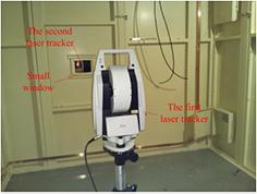
Figure 1. Orientation of two instruments in a situation where there is only a small window between them.
Download figure:
Standard image High-resolution imageFigure 2 (left) illustrates the common technique of connecting a network of laser trackers (triangles) using multiple measurements to points offset from the baselines between them. Figure 2 (right) illustrates the alternative, novel orientation method for two laser trackers to be presented in this paper. This method directly links the instruments using on-board targets and will, for convenience, be called on-board target orientation with 2-face measurement (OBTO2). Where the commonly used method has static orientation targets, the OBTO2 method has targets fixed to the head of the tracker and moving with it. By keeping the targeting close to the baseline between the instrument heads, only a narrow viewing space between the instruments is required. The method is an extension of an existing technique developed for industrial theodolite intersection systems [9, 15] and is related to the geodetic method of traversing used in map making.
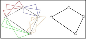
Figure 2. Alternative network constructions.
Download figure:
Standard image High-resolution imageThe remainder of this paper is organized as follows:
- Section 2OBTO2 orientation principle and operation are illustrated, including two-face reciprocal measurement and measurement of baseline length.
- Section 3An accurate model of the method is developed, with an optimized solution to solve it.
- Section 4The OBTO2 is verified through comparison experiments using control points. Uncertainties in experimental results are analyzed by Monte Carlo simulations.
- Section 5Concluding remarks and a brief overview of further planned work.
2. Basic principle
2.1. Two-face reciprocal measurement for theodolite intersection
Like cameras, theodolites can be oriented to one another by sighting multiple targets offset from the baseline which connects their rotation centres. As with cameras, this is the procedure of choice when a single theodolite is moved from measuring station to measuring station in order to complete the measuring task. Where at least two cameras are employed, this technique is still used to establish their relative orientation. However, where at least two theodolites are involved, and are intervisible, an alternative technique can be adapted which is common in map making and civil engineering construction. Here each instrument directly sights to the position of another instrument. This is done using exchangeable targets in which a target replaces a theodolite position. This works for accuracies of millimetres but for metrology the measurement of the baselines must be done using the theodolites themselves as targets.
Figure 3 illustrates the method of reciprocal pointing. Each theodolite sights a target on the moving head of the other theodolite in each telescope position. The relative movement stabilizes quickly to a fixed pointing and the mean of the vector pointings in each face provides the required pointings along the baseline, R1 and R2.

Figure 3. 2-face4 reciprocal measurement with theodolites. (a) 2-face measurement in face 1, (b) 2-face measurement in face 2.
Download figure:
Standard image High-resolution imageTo complete the orientation it is necessary to determine two more vector directions for full angular orientation, and measure a scale length to determine the separation of the theodolites. Figure 4(a) shows two non-levelled theodolites sighting the two end targets on a reference scale-bar. The vector directions V1 and V2 to just one of the scale-bar targets provide the necessary angular information, in this case the roll angle about the baseline. Measurement to the second scale-bar target provides scale information to deduce the theodolite separation.

Figure 4. Roll angle and separation for the relative orientation of two theodolites. (a) Non-levelled, (b) levelled.
Download figure:
Standard image High-resolution imageIf each theodolite is levelled then offset vectors V1 and V2 are not required to establish full angular orientation as this can be done using the known directions of gravity at each instrument, G1 and G2. However, it is important to note that even with levelled instruments it is still necessary to measure an offset scale-bar to establish instrument separation. Achievable accuracies can be around 25 μm–50 μm at 5 m (these values are taken from an out-of-print brochure for the Wild-Leitz RMS2000, a dual-theodolite measurement system now no longer in production).
2.2. Two-face reciprocal measurement for laser trackers
The method of reciprocal pointing can be applied to levelled laser trackers with advantages provided by two additional features:
- The trackers do not require a scale-bar to determine their separation but can use direct distance measurements to a point close to the baseline. This enables them to be relatively oriented in a confined space.
- Unlike the manual procedure required for reciprocal pointing with theodolites, the built-in tracking feature of laser trackers automates the reciprocal pointing process.
It should be noted that if offset targets are attached to arbitrary positions on the heads of the laser trackers, the reciprocal pointing method described above may not result in a fully optimal orientation solution. However, the optimized method presented below avoids this disadvantage. It is emphasized that the technique has value when two laser trackers are available to make the connection between measuring locations and when both can be levelled. However, most modern laser trackers either have built-in tilt sensors or tilt sensors can be added. It is also worth noting that the method could also be applied to total stations which, like laser trackers measure two angles and a distance.
Two Leica AT401 laser trackers were used in the evaluation presented here. Figure 4 shows the laser trackers, identified as L1 and L2, with reflector targets P1 and P2 attached to the respective tracker heads. These reflector targets are subject to any horizontal and vertical movements of the heads. The targets are then measured in two faces as illustrated in order to establish the vector directions between them.
In figure 5(a), both laser trackers are in face 1. After any residual tracking movement has stopped, the offset targets are measured by the observing trackers, and their coordinates recorded. The measured Cartesian coordinates of P2 in the L1 coordinate system are given by  . The index on the upper left identifies the face position (here f1). The index on the lower left identifies which instrument coordinate system defines the coordinate values (here L1). The index on the lower right identifies the target (here 2). Similarly, the measured Cartesian coordinates of P1 in the L2 coordinate system are given by
  .
.

Figure 5. 2-face reciprocal measurement with laser trackers. (a) Both in face 1, (b) both in face 2.
Download figure:
Standard image High-resolution imageIn figure 5(b), L1 and L2 change face and repeat the measurement. Now the corresponding Cartesian coordinates of P2 in the L1 system are given by  , and for P1 in the L2 system by
  .
.
The details of the change of face are shown in figure 6. For approximately horizontal pointings, as was the case here, the horizontal and vertical angles change by approximately 180°.

Figure 6. Technique of changing face.
Download figure:
Standard image High-resolution imageThe unit vector directions between the trackers are calculated as follows. The unit vector to the origin of L2 in the L1 coordinate system is given by:

where  and
and  . Similarly, the unit vector to the origin of L1 in the L2 system is given by:

where  and
and  .
.
As already indicated, with the aid of the internal tilt sensor, the Leica AT401 laser trackers are levelled before measurements and their Z axes are therefore parallel. As a result, the orientation of L2 with respect to L1 has only four degrees of freedom, which can be expressed by a bearing angle θ about the Z axis of L2, and a 3D shift vector T of L2 with respect to L1.
The bearing angle θ is easily estimated from the projections of the two direction vectors on XY plane. Taking unit vector  as the projection of
  on the XY plane, and similarly unit vector
  as the projection of
  , then the bearing angle is given by:

For shift vector T, since its direction can be provisionally defined as  , shift vector T can be expressed as

where d is the length of vector T. Apart from length d, the calculated unit vector directions enable 2 of the 4 orientation parameters to be determined. Separate measurements are made to determine the final parameter d, see next section.
2.3. Distance measurement
As indicated earlier, the magnitude of the shift vector (spatial length of the baseline) is still unknown after the two-face reciprocal measurement. One way to determine this is to introduce a target point P3 located close to the baseline between the instrument centres. Figure 7 shows the two centres and point P3 which together form a triangle. The instrument separation can then be found as follows.

Figure 7. Principle of distance measurement.
Download figure:
Standard image High-resolution imageTarget point P3 sits in a fixed nest, and by manual rotation, it can be measured by both L1 and L2. The Cartesian coordinates of P3 in the L1 coordinate system are given by  , and in the L2 coordinate system by
  . The spatial angles between baseline and target pointings are then given by the vector dot products as:

From the cosine rule, the distance d between the two instrument centres is then:

Here  and
and  are the respective distances from each tracker to P3. The vector shift between the instruments is then given by equation (4).
In this way, all orientation parameters are obtained using measurements to three targets. In addition, all three targets lie close to the connecting baseline between the instruments which reduces the required measurement space.
3. Accurate model and optimized solution
In the previous section, the relative orientation between the trackers is calculated by a direct method which is not fully optimal. Essentially this is because the means of the coupled target vectors in 2-face measurement are not, in general, exactly equal to the direction vectors between the instrument centres. Use of mean vectors is valid for levelled instruments and on-board targets which are vertically offset from the rotation centres, but not where there are lateral target offsets as is the case here (see figure 9). An optimized solution is therefore adopted which uses the results from the direct calculations as initial values.
Take the default coordinates of P1 in the L1 coordinate system as  . In this position the default rotation is at horizontal angle 0° and vertical angle 0° which corresponds to a downward pointing along the instrument Z axis. Similarly, the default coordinates of P2 in the L2 coordinate system are given by
  . These two coordinate values are unknown.
Figure 8 shows the situation with P1 which, for one of the two-face pointings, is rotated by horizontal angle α and vertical angle β. The corresponding transformation matrix is a rotation matrix  expressed as follows:

Figure 8. Transformation of P1 in L1 coordinate system from default to rotated position.
Download figure:
Standard image High-resolution imageThe target coordinates measured by the sighting instrument in the two-face reciprocal measurements can also be given as spherical coordinates. In face 1 of L1, the Cartesian coordinates  is transformed as spherical coordinates
  , where d1 is the slope distance, α1 is the horizontal angle, and β1 is the vertical angle, and their corresponding relationship is expressed as follows:

In this reciprocal measurement situation, as shown in figure 5, the rotated coordinates of P1 in the L1 coordinate system are then given by  , where

Similarly, the Cartesian coordinates  is transformed as spherical coordinates
  . For the reciprocal measurement, the rotated coordinates of P2 in the L2 coordinate system are
  , where

In second face measurement, all the processes are analogous. At the point of reciprocal measurement, the rotated coordinates of P1 in the L1 coordinate system are given by  , and correspondingly the coordinates of P2 in the L2 coordinate system by
  . Here the rotation matrices
  and
and  use the face 2 angle values corresponding to the face 1 angles in
  and
and  .
.
The relationship between these points and the orientation parameters of the two laser trackers can be expressed as:
where

Substituting for  ,
,  ,
,  and
and  in (11), and re-writing, results in:
By eliminating the unknown coordinate values  and
and  , the final simplified set of equations is:
There are 9 equations and 4 unknowns in the set of equations. The equations can be solved using a nonlinear optimization such as the Levenberg–Marquardt algorithm [11]. The results from section 2 can be used as initial iteration values for the optimization.
4. Validation experiments
4.1. Set-up of the experiments
As the true orientation parameters are not known, a common point transformation (CPT) method was used to evaluate the OBTO2 method. The experiment used two Leica AT401 laser trackers and 8 control points for CPT. Taking L1 as the reference station, the coordinates of 8 control points in the L1 coordinate system are listed in table 1. Here points are arranged according to their distance to L1, from about 2.5 m to about 12 m.
Table 1. Coordinates of control points in L1 frame.
| Point No. | x (mm) | y (mm) | z (mm) |
|---|---|---|---|
| 1 | 910.1454 | −2375.9192 | −251.2464 |
| 2 | −2522.5484 | −2945.4809 | −1385.3864 |
| 3 | −7958.6182 | 3046.6142 | 560.9852 |
| 4 | −7710.3259 | −4070.3490 | −1378.0090 |
| 5 | −5919.2764 | −7220.5442 | −222.4040 |
| 6 | 5163.1715 | −7937.7364 | 555.1530 |
| 7 | −5090.8323 | −9864.7563 | −1378.8760 |
| 8 | 11 646.2616 | −151.7258 | 555.5869 |
The 8 control points are then measured by L2 and a closed form solution [12] with global optimization is used to solve for the orientation parameters. Results are shown in the second column of table 2.
Table 2. Orientation results and deviations of OBTO2 compared with CPT.
| CPT method | Basic solution | Optimized solution | |||
|---|---|---|---|---|---|
| Orientation result | Orientation result | Deviation | Orientation result | Deviation | |
| θ (rad) | 2.602 209 | 2.602 214 | 0.9 ('') | 2.602 216 | 1.4 ('') |
| T_x (mm) | −1032.9861 | −1032.9699 | 0.074 |
−1032.9573 | 0.065 |
| T_y (mm) | −4997.3348 | −4997.3403 | −4997.3441 | ||
| T_z (mm) | −83.5891 | −83.5169 | −83.5316 | ||
An OBTO2 experiment was then made between L1 and L2 which were separated by about 5 m. A photo of the experiment is shown in figure 9. Both the basic method, and the optimized method, were used to process the measurement data. The results were evaluated by comparing them with CPT results in the next section.

Figure 9. On-board target measurement experiment.
Download figure:
Standard image High-resolution image4.2. Evaluation of the results
Two methods were used to evaluate the OBTO2 results.
- 1.A direct comparison of orientation parameters between the OBTO2 and CPT solutions.
- 2.Comparison of control points. In the CPT analysis, the 8 control points are also measured by L2. These are transformed by the orientation parameters of L2 which were calculated in the OBTO2 procedure and directly compared with the 8 control point values originally measured by L1. In the absence of errors, these would be identical values.
The OBTO2 orientation results, and deviations compared with those from the CPT method, are summarized in table 2. The coordinate deviations of the 8 control points, transformed by the OBTO2 orientation parameters and compared with the L1 control values, are shown in figure 10.

Figure 10. The 3D coordinate deviations of 8 control points.
Download figure:
Standard image High-resolution image
The experiments demonstrate the feasibility and effectiveness of the approach in this article. Both the basic solution and optimized solution exhibit small deviations with 3D errors of 8 control points below 0.15 mm compared with classical CPT method.
4.3. Uncertainty evaluation by Monte Carlo simulation
According to the measurement uncertainty evaluation guide [13] published by ISO/IEC, Monte Carlo (MC) simulations can be used to estimate the uncertainty of experimental results.
The uncertainty parameters of the Leica AT401 laser tracker, expressed as maximum permissible errors (MPE), are listed in table 3 [10]. Both the basic and optimized methods were simulated with 10 000 samples.
Table 3. Uncertainty parameters of Leica AT401 laser tracker.
| Component | Uncertainty |
|---|---|
| Absolute distance meter's accuracy | ±10 μm |
| Angle accuracy, full range | ±15 μm + 6 μm m−1 (1.2'') |
The orientation uncertainties of the experiment result using the OBTO2 method are shown in table 4 which illustrates the method's high accuracy. The 3D shift uncertainty of the optimized method is about 20% less than that of the basic method. The angle uncertainties of two methods are equal which means the basic method has almost reached the optimal result in angle solution.
Table 4. Uncertainties of orientation parameters by MC simulation.
| Component | Basic method | Optimized method |
|---|---|---|
| 3D shift uncertainty | 46 μm | 38 μm |
| Angle uncertainty | 1.9'' | 1.9'' |
5. Conclusions
The article presents a novel relative orientation method for two laser trackers based on measurements to on-board targets. It is potentially suitable for laser trackers, as well as total stations, which permit mounting of such on-board targets.
The method is a further development of an older theodolite orientation method using reciprocal measurements in both instrument faces. The additional capability of laser trackers to make accurate distance measurements between instruments enhances the original method.
This new method enables an orientation to be made within a restricted measurement environment such as a narrow corridor or where space is limited by a small window connecting the two tracker heads. It is therefore very suitable for use in confined spaces where conventional orientation methods are not easily applied.
Orientation parameters can be calculated directly in a simple geometrical solution and, if required, further optimized in a non-linear optimization.
The validity of the technique has been established by comparison experiments with 8 control points established by a transformation method. Results indicate that 3D coordinate deviations at the 8 control points are less than 0.15 mm. Uncertainties in results have been estimated by Monte Carlo simulation. For the optimized solution, the uncertainty in the 3D orientation parameters is 38 μm and the bearing angle uncertainty is 1.9''. The 3D uncertainty in the optimized solution is around 20% less than in the simple, direct solution. These estimated uncertainties suggest that the method, which is practical, has good accuracy.
The tests also revealed a limitation in the original reciprocal pointing technique for theodolites which means that the use of averaged pointings was strictly only correct for vertically offset on-board targets and levelled instruments. Future work will analyze this in more detail and evaluate two further refinements.
In this paper, the coordinate values of the on-board targets in each tracker are unknown, so during the derivation of optimized solution, these unknown variables are eliminated. However, if the on-board tracker targets are known in the respective tracker coordinate systems by prior calibration then the instruments can be connected using only a single measurement in one face. The calibration technique would also enable the elimination of the third target which was required here to establish the baseline length.
Acknowledgments
This work was funded by the National Natural Science Foundation of China (Grant No. 51305297, 51225505, 51405338) and the Natural Science Foundation of Tianjin (Grant No. 15JCQNJC04600).
Footnotes
- 4
'Face' is a term from surveying technology to indicate which of two possible telescope positions are used for a pointing. These are identified by the 'face' of the vertical angle encoder being either on the left (1) or right (2) of the observer who is looking through the telescope.