
Abstract
To distinguish between chemical bonding and physical binding is usually simple. They differ, in the normal case, in both interaction strength (binding energy) and interaction length (structure). However, chemical bonding can be weak (e.g. in some metallic bonding) and physical binding can be strong (e.g. due to permanent electrostatic moments, hydrogen binding, etc) making differentiation non-trivial. But since these are shared-electron or unshared-electron interactions, respectively, it is in principle possible to distinguish the type of interaction by analyzing the electron density around the interaction point(s)/interface. After all, the former should be a contact while the latter should be a tunneling barrier. Here, we investigate within the framework of density functional theory typical molecules and crystals to show the behaviour of the electron localization function (ELF) in different shared-electron interactions, such as chemical (covalent) and metallic bonding and compare to unshared-electron interactions typical for physical binding, such as ionic, hydrogen and Keesom, dispersion (van der Waals) binding and attempt to categorise them only by the ELF and the electron population in the interaction region. It is found that the ELF method is not only useful for the characterization of covalent bonds but a lot of information can be extracted also for weaker types of binding. Furthermore, the charge integration over the interaction region(s) and tracing the ELF profile can reveal the strength of the bonding/binding ranging from the triple bonds to weak dispersion.
Export citation and abstract BibTeX RIS

Original content from this work may be used under the terms of the Creative Commons Attribution 4.0 licence. Any further distribution of this work must maintain attribution to the author(s) and the title of the work, journal citation and DOI.
1. Introduction
Binding is present in all molecules and solids, which means it is very important for the study of matter. The detailed analysis of the nature of the binding is important especially for complex systems, and is a difficult task using either first principle calculations or experiment. Some of the common theoretical methods that are used for the identification of binding are sensitive to the computational parameters, or are not enough to determine the binding type. In difficult cases, a combination of them is needed or rough approximations have to be used.
Many aspects of binding can be studied using the Bader analysis which is based on a topological analysis of the electron densities [1] where Richard Bader developed an intuitive way of dividing molecules into atoms by using the gradient field of the electron density and is called the quantum theory of atoms in molecules (QTAIM) [1–3]. Another analysis is the charge density difference (CDD) that compares the bound system's electron density with those of the constituents, but it does not solely depend on ground state properties. There is also the non-covalent interaction (NCI) index [4, 5] that analyzes and visualizes the important non-covalent interaction regions by using the densities and its derivatives. Our focus is, however, on another topological analysis; the electron localization function (ELF) introduced by Becke and Edgecombe [6–8]. One important property of ELF is that it involves ground state properties, and thus depends only on the level of approximation of the system (quality of the physical description) and is the link between the quantum mechanical calculations and the understanding of atomic interactions (binding) [9]. Beside the information about the binding, ELF provides also information about the location of bonds, the atomic structure of the system, the electron pairs, and the strength of the bond by integrating the electron density of the ELF region. This can be used to determine if the interaction is of chemical bonding type (covalent bonds, metallic bonds) or of physical binding type [ionic binding, van der Waals binding (including hydrogen-/Keesom-, polarization- and dispersion-binding)].
In this paper, we present the characteristics of ELF for these different types of interactions and their sub-categories in order to find patterns for a direct and easy identification of the interaction type (without using combinations of different methods) completely based on the equilibrium properties of the system. We separate the interactions into two main categories: (i) shared-electron interactions (chemical bonding) and (ii) unshared-electron interactions (physical binding). For the first one, we use examples of typical molecules with known interactions, such as organic small molecules (for the single, double and triple covalent chemical bonds), Al and Cu (for metallic bonds), and mixed covalent and metallic bonds in phenyl bonded to a copper surface. While for the second main category we examine NaCl (ionic binding) and for the van der Waals (vdW) interactions we use the base pairs of AT and GC in DNA (hydrogen binding interaction), Ar⋯HCl (polarization binding interaction), graphene on metal surface (strong dispersion interaction) and graphite (normal dispersion interaction).
The rest of the paper is organized in the following way, in section 2 the computational methods used to characterize the studied systems are presented. In section 3, we discuss the theory behind the ELF and its properties. In section 4, our results are presented followed by our conclusions in the last section 5.
2. Computational details
The properties of the systems were determined via the first-principles calculations using density functional theory (DFT) with the generalized gradient approximation (GGA) by Perdew–Burke–Ernzerhof (PBE) for the exchange–correlation energy [10] implemented within the projector-augmented wave (PAW) method [11, 12] for describing the interaction between the core and the valence electrons in the Vienna ab initio simulation package (VASP) [13–15]. VASP uses an iterative solution of the Kohn–Sham equations within a plane-wave basis while smearing of the electronic occupations with a Gaussian function with the value 0.05 eV. For describing the van der Waals forces we use the dispersion-corrected, semi-empirical PBE-D3 functional proposed by Grimme [16] which is in conjunction with the PBE exchange–correlation functional. We also use the vdW density functional method with optimized exchange term (optB86b-vdWDF) [17] where the results are all in agreement with the PBE-D3 method.
In our systems where molecules are involved (small organic molecules, base pairs and graphene and phenyl on metallic surface), a (1 × 1 × 1) Monkhorst–Pack [18] k-point mesh was used and the vacuum in the supercells was big enough (varies depending on the size of the molecule) to ensure that there was no interaction between periodically repeated molecules in any direction. In the metallic systems, a (15 × 15 × 15) Monkhorst–Pack k-point mesh was used. Furthermore, all the studied systems were allowed to fully relax within the conjugate-gradient algorithm until the force acting on each atom is less than 10−3 eV Å−1. The integration of basins of attractors was done by using the bisector (YT) algorithm [19], which is implemented in the critic2 software [20, 21], while the Virtual NanoLab (VNL) software [22] was used to set up the simulation cells and supercells and the visualization of the ELF has been carried out with VESTA [23].
3. The electron localization function
The topological analysis of the electron density ( ) can with advantage be used to gain chemical information of a molecule or material from first-principles calculations and is related to the Pauli exclusion principle. This theory is known as atoms in molecules (AIM) [2] and incorporates information of critical points of the electron density gradient vector field (
 ) in order to partition a molecular system into atoms. The main advantage of AIM theory is that the electron density is independent of the method by which it has been extracted (although its quality will depend on the level of approximation), is a quantum mechanical observable and may also be obtained experimentally [24, 25] or from Wigner function measurement [26].
Similar to the above mentioned approach is the electron localization function (ELF) and as Becke and Edgecombe [6] said is a 'simple measure of electron localization in atomic and molecular system'. In other words, the ELF is the probability density of finding another electron near the reference electron with the same spin and it is associated with the electron density which means that it shares the many advantages with the Bader analysis. ELF (n(r)) is also a differential scalar field in 3D space (like the electron density p(r)) and its definition is the following:

where χ(r) is the ratio of electron localization D(r) with respect to the uniform electron gas Dh(r):
where the electron localization density is defined as the difference between the kinetic energy density and the bosonic kinetic energy density which is called the von-Weisäcker term. The kinetic energy density is not uniquely defined [27] but this does not affect the result of D(r) as long as in both terms the same definition is used. p is the electron charge density:

The concept is quite similar to the Bader analysis in the sense that the analysis is performed by using the gradient vector field  and looks for its critical points where
  . Those critical points show local maxima, minima and saddle points of n(r). From equation (1) we see that the ELF is dimensionless since the ratio χ(r) is also dimensionless with the only requirement that the definition of the kinetic energy density is the same in both D(r) and Dh(r). In consideration of the arbitrary choice of the reference Dh(r), the ELF is a relative measurement of the electron localization D(r) and it takes values in the range between 0 and 1. In general, it is close to unity in regions occupied by paired electrons where the excess kinetic energy takes low values [28]. When n(r) is high (>0.7), then the electrons are characterized as localized which means for example that there is core or bonding regions or lone pairs. On the other hand, when 0.7 < n(r) < 0.2 the electron localization is similar to the electron–gas and is characteristic for metallic bonds. The localization domains are defined by the isosurfaces of the ELF and they may enclose one or more local maxima (point, ring and spherical attractors). There are three main types of attractors: core (or nuclear), bonding (between two or more nuclei) and the non-bonding (lone pairs), where the two last belong to the more general category of non-nuclear attractors. The ELF index describes in a very successful way the atomic cells and chemical bonds in molecules and solids [6, 7, 29, 30], while it can also give information about systems with physical binding [31, 32]. The ELF of a system can be illustrated through 3D ELF figures, for which an appropriate isosurface value of n, of equation (1), need to be chosen. A suitable value for n can be estimated from 2D ELF cuts through the region(s) of interest, or from an ELF profile plot across the interaction region (see the examples below). But a word of caution is needed for the 3D ELF figures, since they can be deceiving and change quite drastically with different values of the isosurface n. A further analysis which can be useful for giving extra quantitative information about the binding is the integration of the electron density p(r) over the localization domains which offers classification of binding based on non-empirical evidence. For chemical bonding, individual attractor basins can be defined in a similar way to the one used in the AIM theory of Richard Bader. By using the ELF data of the system, the attractor basins are defined by the zero-flux condition of the gradient. Within these basins the electron density is integrated, which gives the number of electrons within.
4. Results
There are mainly two types of atomic interaction, the shared-electron interaction (chemical bonding) and unshared or closed-shell interaction (physical binding). The chemical bonding includes the covalent and metallic bond, where there is always at least one bond attractor, while the physical binding consists of the ionic and van der Waals binding with or without permanent electrostatic moments. We have applied the ELF analysis, and its charge integration over the attraction basins, to a selection of systems to investigate patterns and characteristics that differ chemical bonding from physical binding. In order to find out the distinguishing features for different types of interactions using this commonly implemented analysis tool.
4.1. Shared-electron interactions
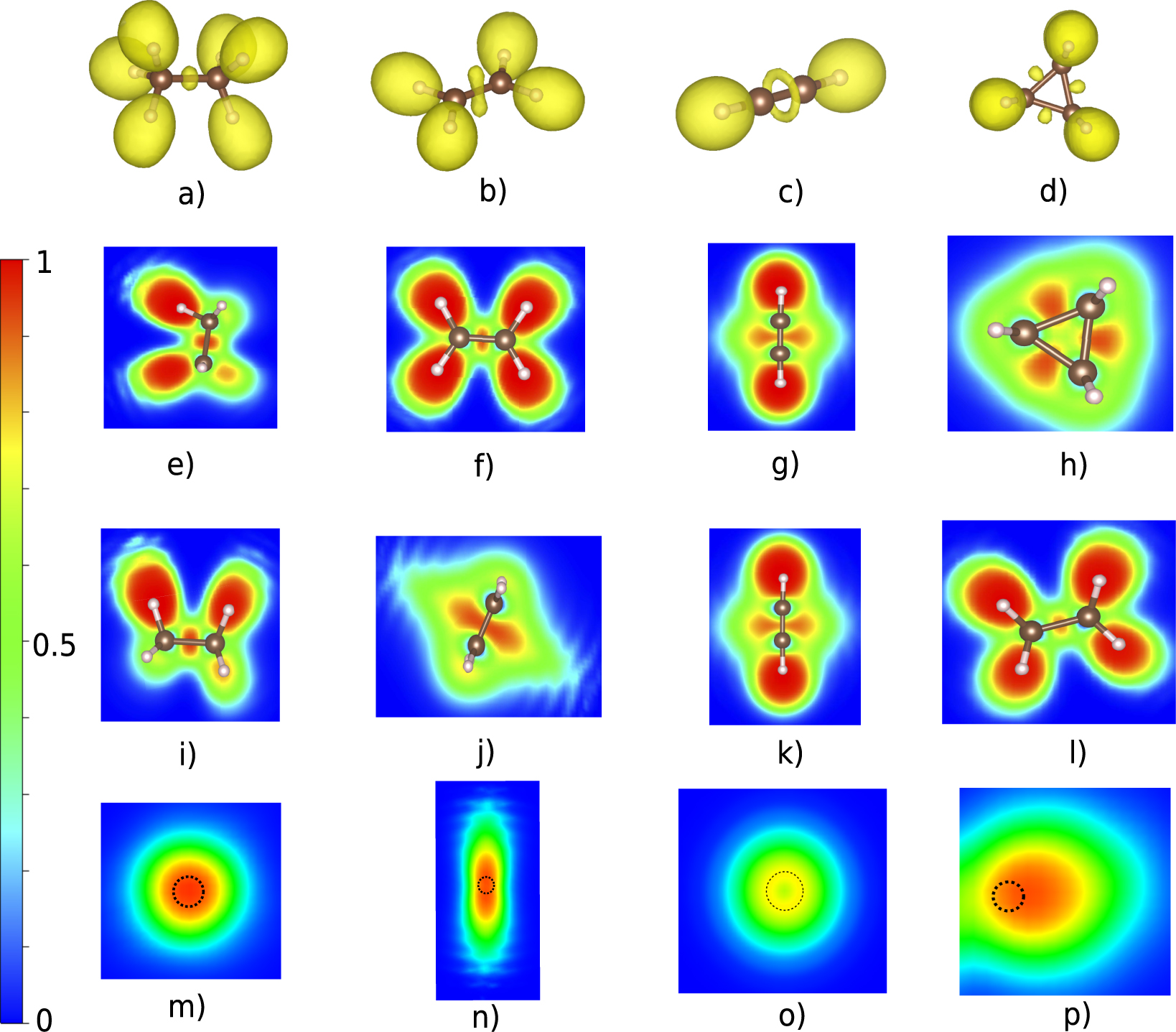
We have used C–C bonds (single, double and triple) as characteristic covalent bonds using the molecules: ethane (C2H6) for a single bond, ethene (C2H4) for a double bond and ethyne (C2H2) for the triple bond as shown in figure 1. We have also studied the so-called 'banana bonds' in the special case of cyclopropane (C3H6). The ELF analysis have been performed and the shape of the ELF in the bond region looks different for each bond type. The C2H6 exhibits a region of highly localized electron density in-between the two C atoms and more precise in the middle of their bond axis and the integrated electron density over this region is 1.8 electrons. The 3D ELF shape of ethane in the bond region is almost spherical shown in figure 1(a), which also can be seen in the 2D ELF of figures 1(e) and (i). This is a characteristic example of how the ELF looks like when a single σ bond is present between two atoms. It also exhibits six ELF basins for the C–H bonds, which always includes the hydrogen atom in question (see figure 1(a)). For the double bond in C2H4 (one σ and one π bond) there is also an ELF basin in-between the two carbon atoms but in this case the shape is different, as shown in figure 1(b). The two overlapping ELF spheres (which can be resolved when n = 0.915) forming a peanut-shaped object where the two lobes are perpendicular to the bond axis, as can be seen from the side view in figure 1(j). The ELF basin contains 3.4 electrons which is considerably bigger than the previous case but less than two times that value. We should mention that in the case of 3D ELF representation, e.g. figures 1(a)–(d), the shape depends on the ELF value n (see equation (1)) and if this value is decreased (increased) then more (less) maxima are shown. As long as the n is high enough then the isosurfaces encloses individual maxima and for the case of ethene gives two maxima for the double bond (n = 0.92) and not one merged as when the value is slightly lower.

Figure 1. The ELF of ethane (single bond), ethene (double bond), ethyne (triple bond) and cyclopropane ('banana' bonds). (a)–(d) 3D representation of ELF with n = 0.88. Top view (e)–(h) and side view (i)–(l) of the 2D ELF. (m)–(p) ELF in the plane perpendicular to the bond axis in the middle of two carbons for each case where the dashed circle shows the position of the bond axis.
Download figure:
Standard image High-resolution imageFor the triple bond in ethyne (C2H2) the ELF basin in-between the carbon atoms is torus shaped (figure 1(c)), which is typical for triple bonds. From the 2D ELF in figures 1(g) and (k) it is easily seen that the three bond domains are degenerate and merged into a torus which means that σ and π bonds separation is not observed, similar to the case of ethene double bond where it is also not possible to observe individually the π and the σ bond. This is clearly shown in figure 1(o), which is the 2D ELF representation of the plane perpendicular to the bond axis, where ELF is zero at the center of the torus. The population of the torus (ELF basin) is 5.3 electrons. We also analyze the special case of 'banana bonds' in cyclopropane (C3H3) with ELF. The localized electrons are not centered on the bond axis but they are found mostly on the outside of the bond axis (figures 1(d) and (h)). This can be seen clearly in figure 1(p) where the dashed circle represents the bond axis. The population of this ELF basin is 1.8 electrons, which is the same as for ethane. The shape of the ELF is however different from the single bond in ethane, as can be seen in the top view (figure 1(h)) that looks almost triangular compare to the rectangular shape in figure 1(e). The ELF description of the cyclopropane bonds is consistent with previous studies [33]. A common ELF characteristic of all these covalent bonds are the non-nuclear maxima which are present in the interaction region. However, the properties of covalent bonds are rather well studied and well understood [34], and the ELF analysis is in agreement with common knowledge.
Another type of shared-electron interaction is the metallic bond which can be described as a partial covalent bond, usually sharing less than one electron [35]. In metals the presence of non-nuclear maxima is also observed in the ELF, like for covalent bonds. However, the interaction region between bonded atoms can also be a weak minimum (see below). The most characteristic feature of ELF for metallic bonds is that the ELF basins are big and extended with uniform localization connecting the atoms of the crystal as illustrated in figures 2(a) and (b) for both Al and Cu unit cells but with different isosurface values, n = 0.6 for Al and n = 0.25 for Cu. One explanation for this quite big difference in ELF value of the interstitial region is the occupation of the 3d orbital [36, 37] where the Al has zero electrons and on the other hand Cu has fully occupied the 3d orbital (10 electrons). We have also calculated the ELF of some other metals, and for the transition metals Fe and V, which have 6 and 3 electrons in the 3d orbital n ∼ 0.35 and n ∼ 0.5, respectively. Our results confirm the influence that the occupation of the d-orbital has on the ELF since their values are in-between Al and Cu.

Figure 2. The ELF of Cu (a) and Al (b). The isosurfaces have been chosen to be n = 0.25 and n = 0.6 for the Cu and Al, respectively. (c) The ELF profile of the interaction regions between neighbouring atoms of Cu (black) and Al (red) along the dashed line shown in (a) under the name 'profile 1' and (d) along the other dashed red line under the name 'profile 2'.
Download figure:
Standard image High-resolution imageOur simulations show that the most characteristic feature of ELF for metallic bonding is the smoothness and that it is almost constant in the interaction regions as can be seen from the ELF profiles of Al and Cu metals along different directions in figures 2(c) and (d). We note here that in the PAW method only valence electrons are taken into account in the calculation and this is the reason for the zero value in the ELF profile in the core of the atoms.
For the identification of metallic bonding the localization window concept can be used. The localization window is nothing else but the difference between the maximum ELF value and the first order saddle point and is a 'tool' which quantifies the smoothness of the ELF along the bond axes. A metallic system is described by an ELF peak value in the 0.2–0.7 range and by a narrow localization window [35], which is 0.02 for the Al, while for the Cu case is 0.04.
There are also cases with mixing of covalent and metallic bonding, for which the bonds and their placements/directions are less intuitive. A good example is provided by the analysis of metal-coordination bonding using ELF for ferrocene [38]. We show phenyl bonded to Cu(111), see figure 3. In this case the bond between the molecule and the metal goes from the C atom to the center of a Cu–Cu metallic bond, as seen in figure 3(b), which shows the faint metallic bonding in the 2D ELF of Cu contrasted by the bright covalent bonds involving phenyl. The corresponding ELF profile for this bond (see figure 3(c)) has the typical shape of a covalent bond, but goes down to the Cu metallic bond value around n = 0.2 at the metal side. The region of highest ELF is thickest towards the Cu–Cu bond center but it is wide, which means that similar ELF profiles can also be traced between the C atom and the two Cu atoms.

Figure 3. (a) The structure of phenyl molecule on Cu(111) surface. (b) 2D ELF along the plane containing the chemical bond between C and a Cu–Cu metallic bond. (c) The ELF profile from C to in-between the two Cu atoms as indicated by the black dashed line in (b).
Download figure:
Standard image High-resolution imageThe distances between the atoms of interest in all the systems that have been studied for the shared-electron interactions are listed in table 1 alongside a comparison to the corresponding theoretical covalent and vdW lengths from adding the atomic covalent and vdW radii. As expected, in all the cases, the computed distances are much shorter than the sum of vdW distances (rvdW). The C–C bond distances of ethane and cyclopropane are very close to the sum of covalent atom radii value (rcov) while the ones of ethene and ethyne are shorter, since they are double and triple bonds. The two last bond distances of table 1 that correspond to the metallic Cu–Cu and Al–Al interactions are in-between the sum of the covalent (rcov) and vdW (rvdW) but closer to the covalent ones, which is expected since metallic bonds are strong interactions but not as strong as covalent bonds.
Table 1. Closest distances of the shared-electron systems in figures 1, 2 and 3. Comparison with the sum of covalent radii (rcov) and van der Waals radii (rvdW). The difference in Å of the calculated distance and the sum of theoretical covalent and vdW values are presented as well.
| Bond (system) | Distance (Å) | Sum of rcov (Å) | Δcov (Å) | Sum of rvdW (Å) | ΔvdW (Å) |
|---|---|---|---|---|---|
| C–C (ethane) | 1.54 | 1.5 | +0.04 | 3.54 | −2.00 |
| C=C (ethene) | 1.33 | 1.5 | −0.17 | 3.54 | −2.21 |
| C=C (ethyne) | 1.21 | 1.5 | −0.29 | 3.54 | −2.33 |
| C–C (cyclopropane) | 1.51 | 1.5 | +0.01 | 3.54 | −2.03 |
| C–Cu (phenyl–Cu(111)) | 1.72 | 1.87 | −0.15 | 4.15 | −2.43 |
| Cu–Cu (Cu bulk) | 2.57 | 2.24 | +0.33 | 4.76 | −2.19 |
| Al–Al (Al bulk) | 2.85 | 2.52 | +0.33 | 4.50 | −1.65 |
4.2. Unshared-electron interactions
In this section, we study the ELF and its ρ electron population in systems where there is no sharing of electrons between the interacting atoms. Such A–B interactions are frequently studied using CDD that can give results that are hard to interprete since it depends on the density of the separated constituents at frozen structures (A* and B*), especially when the interaction is unusually strong or very weak. On the contrary, the ELF analysis only depends on the ground state properties of the A–B system. A typical unshared-electron interaction is the ionic binding represented by NaCl. Due to the lack of electron sharing the ELF in the region between the nuclei of the atoms is characterized by very low values (below 0.01. See also the ELF-profile in figure 5(c)). On the other hand, there is high localization around the anion [39] as can be seen in figures 4(b) and (c). Figure 4(d) shows the high localization region of an isolated Cl atom that has spherical shape. However, the shape of the ELF for Cl− in NaCl is distorted, as can be seen there are six very smooth edges around the ELF basin, four shown in figure 4(b) and the other two in figure 4(c). These point towards the six neighbouring Na atoms. This shape distortion of the ELF basin can be seen clearer from the ELF profiles (figure 5(c)), which are taken along two different directions of the horizontal planes that are shown by the black and red arrow in figure 5(a) and compare to the isolated Cl atom. We observe that in the case of horizontal plane the ELF basin is not symmetric and the profile shown along the Cl⋯Na direction (red arrow in figure 5(a)) is broader (red line of figure 5(c)) than the Cl⋯Cl direction (black line figure 5(c)), which shows the appearance of the previously mentioned very smooth edges in the ELF shape. Both of these profiles are narrower than the one of the isolated Cl atom (blue line figure 5(c)), although we are comparing Cl− in NaCl with a neutral Cl atom, due to the presence of the Na atoms in the NaCl system. Such contraction is evidence of an ionic interaction between the Cl and Na atoms (or in other cases van der Waals interaction, see below). The binding length is much shorter than the sum of rvdW (see table 2), since the radii should be for Na+ and Cl− not the neutral atoms. Ionic binding is strong and clearly has no sharing of electrons, which is seen easily from the ELF analysis.
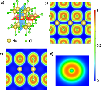
Figure 4. (a) The horizontal (red) and vertical (blue) planes of the NaCl salt. (b) The 2D ELF of the horizontal plane and (c) of the vertical plane. (d) The 2D ELF of an isolated Cl atom.
Download figure:
Standard image High-resolution image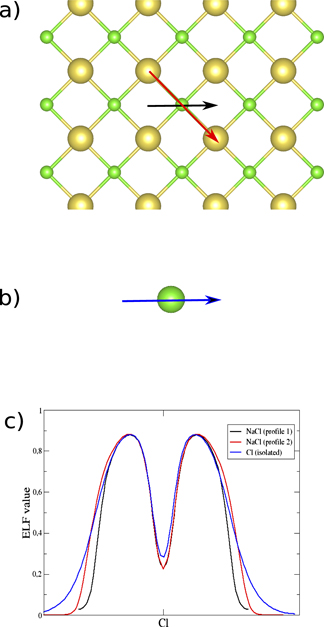
Figure 5. (a) The horizontal plane of the NaCl system where the directions of the ELF profiles are shown by the black and red arrow. (b) The blue arrow demonstrate the direction of the ELF profile of the isolated Cl atom. (c) The ELF profiles of the Cl atom for different directions in the horizontal plane (black and red lines) and of the isolated Cl atom (blue line).
Download figure:
Standard image High-resolution imageTable 2. Bond distances of the unshared-electron systems in figures 4, 6, 9 and 10. The theoretical corresponding covalent (rcov) and vdW (rvdW) radii of each element are also shown along with their difference from the calculated distance.
| Binding (system) | Distance (Å) | Sum of rcov (Å) | Δcov (Å) | Sum of rvdW (Å) | ΔvdW (Å) |
|---|---|---|---|---|---|
| Na⋯Cl (NaCl salt) | 2.81 | 2.54 | +0.27 | 4.32 | −1.51 |
| N⋯H (adenine–thymine) | 1.74 | 1.03 | +0.71 | 2.86 | −1.12 |
| H⋯O (adenine–thymine) | 1.74 | 0.95 | +0.79 | 2.70 | −0.96 |
| H⋯O (guanine–cytosine) | 1.84 | 0.95 | +0.89 | 2.70 | −0.86 |
| H⋯N (guanine–cytosine) | 1.80 | 1.03 | +0.77 | 2.86 | −1.06 |
| O⋯H (guanine–cytosine) | 1.61 | 0.95 | +0.66 | 2.70 | −1.09 |
| H⋯Ar (Ar⋯HCl system) | 2.64 | 1.28 | +1.36 | 3.03 | −0.39 |
| C⋯Cu (graphene–Cu surface) | 3.02 | 1.87 | +1.15 | 4.15 | −1.13 |
| C⋯C (graphite) | 3.42 | 1.5 | +1.92 | 3.54 | −0.12 |
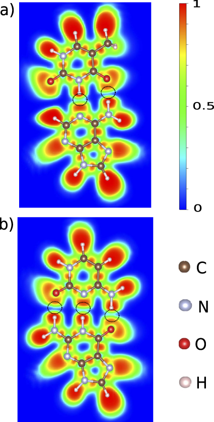
Physical binding that involve permanent dipole moments (or bond dipoles), as exemplified by hydrogen binding, plays a very important role in the inter- and intra-molecular interactions as well as in the structures and properties of matter. The ELF has been used in the past in order to characterize the strength of the hydrogen binding (weak, medium and strong) [31, 32]. We study the case of intermolecular hydrogen binding in the DNA base pairs (adenine–thymine, guanine–cytosine), which are typical examples of this kind of interaction where the topological analysis of ELF can provide clear results. Despite the fact that the hydrogen binding is considered weak the complementary base pairs provide great stability and this comes from the number of hydrogen bindings in the complexes, two between adenine and thymine and three between the guanine and cytosine which are shown with black dashed circles in figure 6. The binding mechanism is through the local permanent dipole moments created by the lone pairs of O or N interacting with the N–H local moment of the other base [40–43]. The two hydrogen bindings of adenine–thymine pair are taking place between the nitrogen and NH2 of adenine and NH and CO of thymine, respectively. Since there is no covalent bond involved, as expected there are no localized regions in between these molecules, but on the other hand their respective basins are very close or even touching and this indicates hydrogen binding. In the case of the guanine–cytosine base pair the regions of hydrogen interaction are three and are taking place between the NH2, NH and O of guanine and the O, N and NH2 of cytosine, respectively. In two out of three hydrogen bindings the two basins are touching, which is interpreted as strong interaction, while in the third one these regions are very close but not as close as the other two. However, in this last case, there is still no clear dark blue region in between which is an evidence of strong interaction but weaker than the other two. By comparing the hydrogen binding interaction regions in figure 6 with other N–H/O–H and lone-pair ELF basins at the perimeter of the two base pairs it is clear that each basin involved in binding is considerably contracted along the interaction direction. Such contractions are characteristic for all types of physical binding, and is particularly pronounced for hydrogen binding. By looking at the ELF profiles along the hydrogen binding it is possible to compare the strength. The ELF profiles are shown in figure 7 where the minimum n corresponds to the region between the bases (marked with dashed black circles in figure 6). In figures 7(a) and (b), the A–T base pair ELF profiles of N⋯HN and NH⋯OC interactions are shown, where their lowest ELF values in the interaction region are 0.31 and 0.17, respectively, concluding that the N⋯HN interaction is stronger. Similar to the AT base pair, the strongest hydrogen interaction of the GC base pair is between the guanine's O and cytosine's H where ELFmin = 0.28 while for the other two interactions the minimum ELF values are 0.138 (guanine's H and cytosine's O) and 0.26 (guanine's H and cytosine's N) as shown in figures 7(c)–(e). Hydrogen binding is considerably strengthened by the mutual alignment of dipole moments, as is clearly seen in the interaction distances that are ∼1 Å shorter than the sum of rvdW (see table 2). Hydrogen binding has its generalization for physical binding that involves permanent moments but not hydrogen atoms (sometimes called Keesom interaction). Although these values of n are comparable to metallic bonding, there is a large difference in the profiles (cf figures 2(c) and 2(d)). For hydrogen binding there is touching of two larger density regions, while for metallic bonding there is an extended region between the atoms with smooth/constant density, a more or less constant value for the localization window. Hydrogen (Keesom) binding is the strongest of the vdW type binding with ELF characterized by contractions of the individual ELF basins on each side of the interaction region, a sharp (V-shaped) minimum in-between with a considerable value of n (above 0.1).

Figure 6. The 2D ELF of the two base pairs. (a) Adenine⋯thymine base pair with the two hydrogen bindings between them and (b) guanine⋯cytosine with the three hydrogen bindings.
Download figure:
Standard image High-resolution image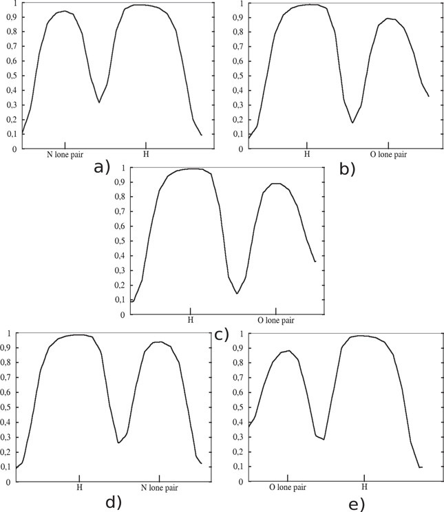
Figure 7. ELF profiles of the five hydrogen bindings of the two base pairs (adenine–thymine and guanine–cytosine). The ELF profile is given along the line of adenine's N lone pair and thymine's –NH (a), of adenine's NH2 and cytosine's O (b). For the guanine–cytosine pair it is shown the ELF profile along the guanine's NH2 and cytosine's O (c), guanine's NH and cytosine's N (d) and guanine's O and cytosine's NH2 (e).
Download figure:
Standard image High-resolution imageApart from hydrogen binding with dipole–dipole interaction (generally multipole–multipole interaction), there is another class of physical binding between two entities where there is one dipole (multipole) that induces a dipole (multipole) due to the interaction, also called induction or polarization binding. Our example for the dipole–induced dipole interaction is the Ar⋯HCl system. The polar covalent bond in H–Cl results in a dipole moment where the negative and positive partial charges are at the Cl and H atom, respectively. When the polar HCl molecule comes close to the spherically symmetric Ar atom its electron density is shifted to one side of the nucleus and it is not homogeneously distributed anymore. This distortion in the electron distribution causes an induced dipole moment on the Ar atom, which strengthens the attraction force between the dipole (HCl) and Ar. An important difference compared with the permanent moments for hydrogen binding (Keesom) is that the induced moment is on an atom and not a bond dipole or due to a lone-pair pointing in a certain direction. The equilibrium geometry is found to be linear. Like for the hydrogen binding case before, there is no localized electron basin between the HCl molecule and the Ar atom (figure 8(c)) as expected due to the lack of covalent bonding. On the other hand, the difference with the previous case of hydrogen binding is that the ELF is much lower between HCl and Ar which is obvious by looking at the ELF profile (black line in figure 8(a)) where the ELF value n is 0.05, but still resulting in a deep blue ribbon in-between in the 2D ELF (see figure 8(b)). This weak interaction can be better identified from the shape of ELF rather than the value itself, in other words the ELF shape changes because of the interaction (contractions). In figure 8(d), the ELF shape of the free Ar atom is a perfect circle in 2D while in figure 8(b) it is not a perfect circle anymore but it is contracted at the side which is neighbouring the HCl molecule. The same contraction of ELF is observed also at the H atom of the HCl molecule (see figures 8(b) and (c)). Induction/polarization binding has similar ELF characteristics as hydrogen binding with basin contractions and a pronounced minimum, but not as sharp and with lower value of n.

Figure 8. (a) ELF profiles of the Ar⋯HCl (black line), free Ar atom (red line) and free HCl molecule (blue line). It is also shown the 2D ELF of Ar⋯HCl (b), free HCl molecule (c) and free Ar atom (d).
Download figure:
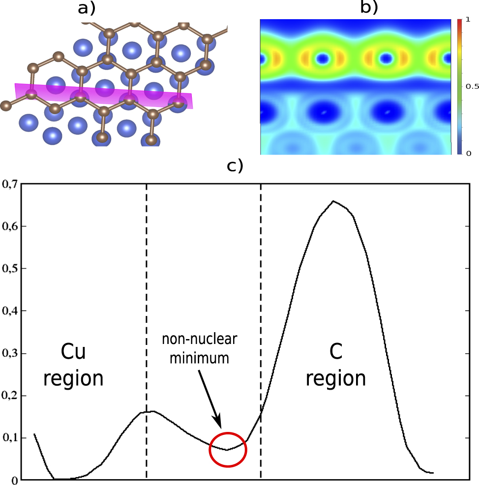
Standard image High-resolution imageAnother type of physical binding is dispersion (sometimes called vdW interaction) that play a crucial role in the structure of molecules and their binding with each other and surfaces [44, 45], which means that they have to be considered in the study of matter [46–48]. Dispersion is due to induced dipole (multipole) moments, and it turns out that there are two types—strong and normal dispersion. An example of strong dispersion is between organic molecules and metallic surfaces [49–51]. We investigate the system of a graphene layer on the Cu(111) surface (figure 9) [52–54]. We compare with graphite (figure 10) as an example of normal dispersion, which is characterized by n very close to zero at the minimum (figure 10(d)), resulting in a deep blue region between the carbon sheets in the ELF plot (figure 10(a)). Normal dispersion has similar ELF and profile as ionic binding, although it is due to induced dipole–induced dipole interactions, with contractions of the electron density of the two interacting entities. However, for the strong dispersion (figure 9(b)) there is still a deep blue region between the carbon sheet and the Cu-substrate, but with a slightly larger density at the touching point (n ≈ 0.07). The interaction is clearly stronger than the normal dispersion in graphite, although there are no bond dipoles or other multipoles in the two binding entities. This is also evident from the binding distance being considerably shorter than the sum of the rvdW—typically in the range 0.5–1 Å shorter (see table 2). For normal dispersion the binding length is comparable to the sum of rvdW, naturally since this is an example of what is normally called vdW binding. The behaviour of the ELF profile for strong dispersion is similar to the ones of the hydrogen interactions presented earlier, although it originates without the permanent dipole (multipole) moments. The induced dipoles are redistribution of electron density on the interacting atoms (as for Ar in the induction binding) that are particularly large. This is attributed to the pliable flexibility of the metallic bonding density of Cu, in this particular example. It is, however, not present in all dispersion between C and Cu (see, e.g. [52]). The emergence of strong or normal dispersion between a particular pair of atoms in physisorption is situation dependent, and is a subject of present research.

Figure 9. (a) Graphene layer on top of Cu(111) surface and the plane for the ELF investigation. (b) 2D plot of ELF for the system and (c) the ELF profile along the interatomic axes of graphene's C and surface Cu.
Download figure:
Standard image High-resolution image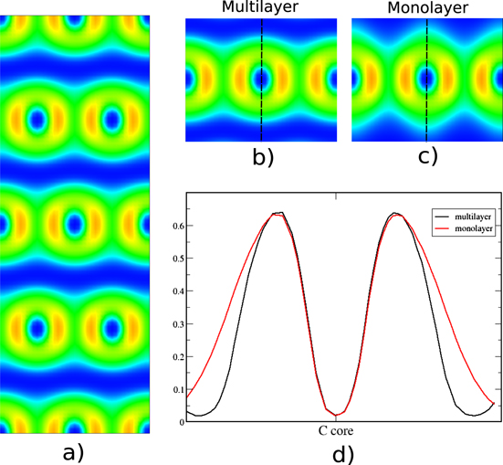
Figure 10. (a) The perpendicular 2D ELF of graphite layers, (b) zoomed-in figure of the multilayer graphite, (c) calculated ELF of graphite's monolayer and (d) ELF profiles of graphite's multilayer (black) and monolayer (red).
Download figure:
Standard image High-resolution image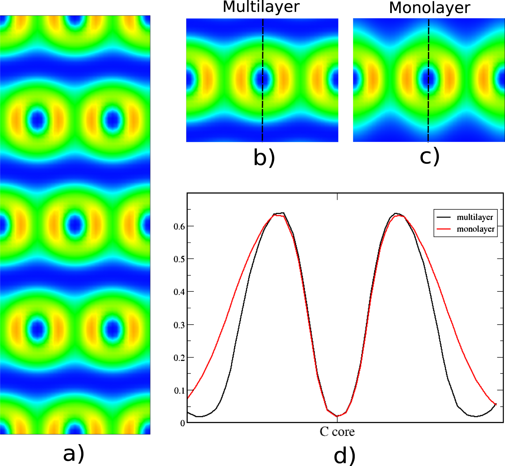
In graphite, the induced dipole results in some contraction of the electron density of each layer. This can be seen in the ELF comparison of a graphite layer with graphene (see figures 10(b) and (c)). This is seen more clearly in the ELF profile plots of figure 10(d) where the monolayer's profile (red line) is broader and is approaching the minimum value slower, further away from the core. The individual ELF basin contractions along all paths of physical binding is a result of the Pauli repulsion which is manifested when electronic states are close to each other without mixing/bonding.
5. Conclusions
ELF analysis, compared to bond order indices, partial and total DOS and charge density difference plots, is by far a better and more universal tool for delving into the essence of interactions either chemical bonding or physical binding. The advantages of using the ELF method for describing chemical bonds are well known but in this work we show that there are clear ELF characteristics ensuring that weaker interactions also can be identified using this tool. By calculating the ELF of typical known systems we have cataloged the differences in ELF patterns for different bonds and bindings which can be used for qualitatively analysis of interactions in unknown systems, resulting in an analysis tool that can be trusted since the ELF depends only on the systems ground state properties.
By calculating the ELF of small organic molecules we show that it is possible to come to a conclusion of the chemical bond type and order (single, double etc) by examining the ELF shape along the interacting atoms, even in special cases of strained/bent bonds, and unconventional mixed covalent and metallic bonding. Moreover, the bond recognition can be strengthened by integrating the charge of the ELF basin in-between the atoms, which will give the number of electrons that are involved in the bond. We also show that the identification of metallic bonds by studying the ELF arises from the size of the ELF basins which is very big and extends in a three-dimensional network in the space between the atoms. The ELF is also smooth and almost constant in that region which results in a very narrow localization window.
Despite the fact that ELF is an excellent tool to identify chemical bonds it is not used to analyze unshared-electron interactions although these are characterized by the absence of localized electrons between the interacting atoms. In this work we present the ELF characteristics for non-covalent interactions (physical binding). For ionic binding we have studied NaCl and show by comparing the ELF of an isolated Cl and the Cl− atom of NaCl that there is a contraction of the ELF of the Cl− (its ELF profile is narrower). On the other hand, when physical binding involves permanent dipole moments (hydrogen binding) or strong dispersion (e.g. graphene on Cu(111)) then the regions with intermediate value of ELF around the atoms of interest are close to each other (in some cases they are even touching) which results in a non-zero ELF in the region in between. Moreover, it is possible to compare the strength of hydrogen bindings by studying their ELF profiles. For weaker interactions, such as dipole–induced dipole or induced dipole–induced dipole interaction, the regions with intermediate ELF value around the interacting atoms are not very close to each other so the ELF shape and how it changes is similar to ionic binding. The ELF is contracted on each side of the region where the binding is taking place.
Acknowledgments
We would like to thank the Swedish Research Council (VR), Knut and Alice Wallenberg Foundation, Kempe Foundations, Länsstyrelsen Norrbotten and Interreg Nord for financial support. We are grateful for allocation of time and resources at High Performance Computing Center North (HPC2N), National Supercomputer Center in Linköping (NSC), and the PDC Center for High Performance Computing, through the Swedish National Infrastructure for Computing (SNIC).