


Abstract
We report distinctly double-peaked Hα and Hβ emission lines in the late-time, nebular-phase spectra (≳200 days) of the otherwise normal at early phases (≲100 days) type IIP supernova ASASSN-16at (SN 2016X). Such distinctly double-peaked nebular Balmer lines have never been observed for a type II SN. The nebular-phase Balmer emission is driven by the radioactive 56Co decay, so the observed line profile bifurcation suggests a strong bipolarity in the 56Ni distribution or in the line-forming region of the inner ejecta. The strongly bifurcated blueshifted and redshifted peaks are separated by ∼3 × 10³ km s−1 and are roughly symmetrically positioned with respect to the host-galaxy rest frame, implying that the inner ejecta are composed of two almost-detached blobs. The red peak progressively weakens relative to the blue peak, and disappears in the 740 days spectrum. One possible reason for the line-ratio evolution is increasing differential extinction from continuous formation of dust within the envelope, which is also supported by the near-infrared flux excess that develops after ∼100 days.
Export citation and abstract BibTeX RIS
1. Introduction
Hydrogen-rich, core-collapse supernovae (CCSNe), also known as type II SNe, originate from massive stars (M ≥ 8 M⊙) that have retained most of their hydrogen content at the time of explosion. From spectropolarimetry studies, CCSNe ejecta are often found to show a significant degree of asymmetry (see, e.g., the review by Wang & Wheeler 2008). In the early photospheric phase of SNe II, the inner ejecta is mostly obscured by the thick and extended envelope of ionized hydrogen, which become increasingly transparent as the ejecta expands and the hydrogen recombines. The late-time, "nebular-phase" observations are particularly important for unveiling the structure of the inner regions once the ejecta becomes optically thin. During the late-time (≳100–150 days) light curve tail, the optical radiation is primarily powered by the decay of radioactive 56Co (the decay product of 56Ni synthesized in the explosion), and the 56Ni distribution in the ejecta can be reflected in the nebular Balmer emission line profiles (Chugai 2007), which can be a powerful probe of the explosion asymmetry. Despite decades of studies of SNe II, the exact mechanism driving the shock within the supernova (SN) during the explosion is still a topic of debate (see, e.g., Janka 2012; Kushnir & Katz 2015; Pejcha & Thompson 2015, and references therein), and non-sphericity and jets are often suspected to be critical for these explosions (e.g., Khokhlov et al. 1999; Janka 2012; Piran et al. 2019; Soker 2018). Studying the asymmetry of the ejecta, especially the inner region, may provide important clues for understanding the explosion mechanism.
CCSNe may be an important source of dust in the universe (see, e.g., Gall et al. 2011). During the nebular phase, as the ejecta cools the gas may start to condense into dust grains and thereby increase the extinction locally. Dust formation has been observed in several CCSNe (e.g., Sugerman et al. 2006; Mattila et al. 2008; Kotak et al. 2009; Inserra et al. 2011; Meikle et al. 2011; Stritzinger et al. 2012; Maeda et al. 2013). The effect of newly formed dust can be manifested in the light curves and spectra of the SN. The dust absorbs the light and re-emits in infrared (IR), resulting in strong IR excess. Substantial dust formation may also lead to asymmetries in nebular emission lines due to differential extinction, as the light coming from the far side of the ejecta suffers more extinction.
Here we present detailed observations of the normal type IIP SN ASASSN-16at until its late nebular phase (up to ∼900 days). ASASSN-16at shows a unique double-peaked profile in Hα and Hβ nebular emission lines, where the relative strengths of the two peaks evolve with time. Such a distinct double-peaked structure is unprecedented for an SN IIP. Huang et al. (2018) studied the near-ultraviolet (NUV)-optical light curves and optical spectra of ASASSN-16at until the early radioactive decay tail phase, showing key features that are typical for a SN IIP. They also reported that the Hα emission profile showed weak asymmetry in their last spectrum at 142 days, for which they suggested three possible interpretations—circumstellar medium (CSM) interaction, asymmetry in the line-emitting region or bipolar 56Ni distribution. Our still later nebular-phase spectra taken at ≳200 days show Balmer lines with double-peaked profiles, which most likely suggest a bipolar distribution of the inner ejecta. Our work focuses on the nebular data, while our full photometry and spectroscopic data are given in the Appendix.
2. Observations
ASASSN-16at was discovered in the host galaxy UGC 08041 by the All-Sky Automated Survey for Supernovae (ASAS-SN; Shappee et al. 2014) on UT 2016 January 20.59 using the "Brutus" telescope in Haleakala, Hawaii (Bock et al. 2016; Holoien et al. 2017). The first ASAS-SN detection was at V = 16.81 ± 0.26 mag on UT 2016 January 19.49, and the last non-detection was V < 18 mag on UT 2016 January 18.35. We adopt the explosion epoch of 2016 January 18.92 (JD 2457406.42 ± 0.57) and use this as the reference epoch throughout this Letter. The host galaxy distance is 15.2 ± 3.0 Mpc according to Sorce et al. (2014; Tully–Fisher distance). We ignore any host-galaxy extinction as we do not detect any Na i D absorption in the SN spectrum, which is consistent with the fairly isolated location of the SN in the outskirts of the host galaxy. We adopt a total line-of-sight reddening entirely due to Milky Way of E(B − V) = 0.019 mag (Schlafly & Finkbeiner 2011) and RV = 3.1.
We obtained NUV through near-IR (NIR) photometry and optical spectroscopy of ASASSN-16at from 0.6 to 881 days. The NUV observations were obtained with the Neil-Gehrels-Swift-Observatory Ultraviolet/Optical Telescope (UVOT). X-ray observations were obtained using the Swift X-Ray Telescope (XRT) and Chandra. We summarize our optical photometric and spectroscopic observations in the Appendix, the photometric results are reported in Table 2, and logs of the spectroscopic observations are given in Table 3.
3. Results
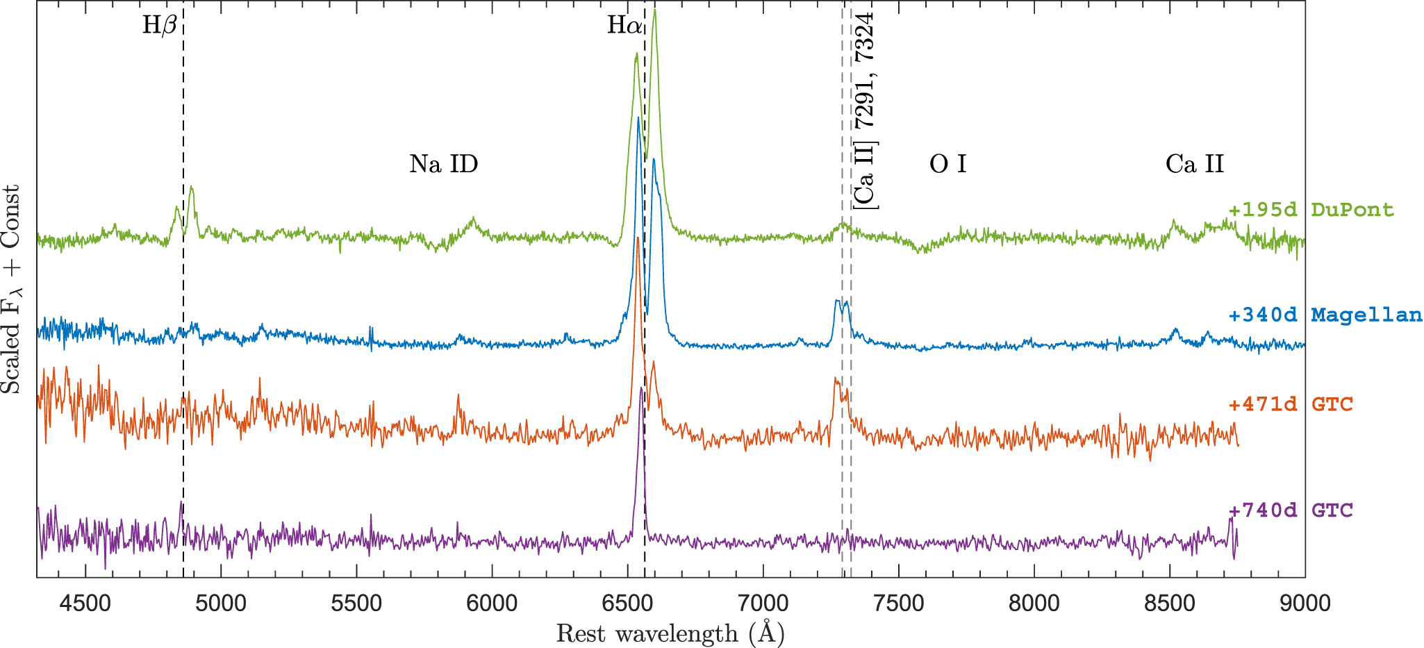
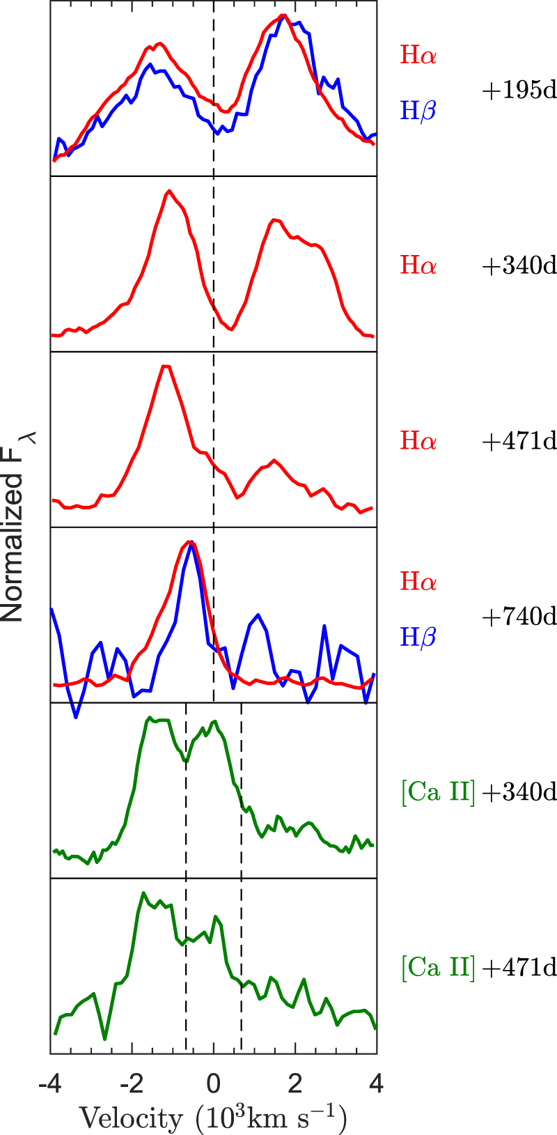
Optical spectra were obtained from 2 days to a late nebular phase of 740 days. We find that the early-phase (≲100 days) spectroscopic properties of ASASSN-16at are typical for a normal SNe IIP, in agreement with Huang et al. (2018). However, the nebular spectra taken at ≳200 days make this SN IIP exceptional. Figure 1 shows the nebular-phase spectra of ASASSN-16at at 195, 340, 471, and 740 days. Starting from 195 days, which is ∼100 days after the onset of the radioactive tail phase, the Hα and Hβ emissions show a very unusual double-peaked profile, where the two peaks, separated by ∼3 × 10³ km s−1, are positioned almost symmetrically in velocity with respect to the rest frame of the host galaxy. Among the two components, the relative strength of the red component is seen to be progressively decreasing with time relative to the blue component (see Figure 2). At 740 days, the red component is no longer detectable, whereas the blue component of both Hα and Hβ remains visibly strong, albeit narrower and shifted closer to the rest frame than in the earlier spectra. See Table 1 in the Appendix for the parameters estimated from the Hα and Hβ line profiles. The Hα emission line is detected in all of the nebular spectra, while Hβ is not clearly seen in the spectra taken at 340 and 471 days, both of which have a relatively low signal-to-noise ratio. The other nebular lines detectable in these spectra are Na i D (λ5890), O i (λ7774), Ca ii triplets (λλ8498, 8542, 8062), and the strong emission of [Ca ii] (λλ7291, 7324).

Figure 1. Deep nebular spectra of ASASSN-16at at four epochs (195, 340, 471, and 740 days). The vertical dashed lines mark the rest wavelengths of the Hα, Hβ, and [Ca ii] doublet.
Download figure:
Standard image High-resolution image
Figure 2. Hα, Hβ, and [Ca ii] nebular lines shown in the velocity domain with respect to the rest wavelengths of Hα, Hβ, and an average of the [Ca ii] doublet. The vertical dashed lines mark the positions of zero velocity for Hα, Hβ, and the [Ca ii] doublet.
Download figure:
Standard image High-resolution imageThe photometric light curves span from 0.6 to 881 days and are shown in Figure 3. Huang et al. (2018) presented NUV and optical light curves up to 170 days, and our photometric measurements during this period are consistent with their results. The NUV, optical, and NIR light curves show the typical evolution of SN IIP, except in the late nebular phase (≳500 days), where the light curves decline more slowly than the typical SNe IIP, especially in the g- and r-bands. The flux contamination from the host galaxy may not be entirely negligible at this very late phase, but our analysis using archival Pan-STARRS1 images (Chambers et al. 2016) suggests that the observed flattening is mostly intrinsic to the SN.

Figure 3. Photometric evolution of ASASSN-16at in the Swift NUV, optical BVugriz-bands, and NIR K-band. Epochs of spectral observations are marked by vertical bars at the bottom, and the four nebular spectra showing double-peaked emission are marked in blue. Within 200–500 days, all of the light curves declined at a faster rate than radioactive 56Co decay, which is illustrated only for the r-band by a red dashed line representing 56Co decay rate.
Download figure:
Standard image High-resolution imageASASSN-16at was observed in 0.3–10 keV using the Swift and Chandra XRT during 2–18 days (see Figure 7 in Appendix). The X-ray luminosity during the initial phases of 2–5 days is about 25 × 1038 erg s−1, which is around the typical luminosity for SNe II with X-ray detections (see, e.g., Pooley et al. 2002; Dwarkadas & Gruszko 2012). However, the luminosity declined to 5 × 1038 erg s−1 by ∼19 days.
4. Discussion
Some SNe II show a certain level of asymmetry in their nebular Hα emission, and a bipolar or asymmetric distribution of radioactive 56Ni in the inner ejecta has been invoked as a possible interpretation. Some notable SNe with nebular Hα asymmetries include SNe 1987A (Utrobin et al. 1995), 1999em (Elmhamdi et al. 2003), 2004dj (Chugai et al. 2005; Chugai 2006), 2012A (Tomasella et al. 2013), and 2013ej (Bose et al. 2015a; Utrobin & Chugai 2017). However, none of the SNe IIP observed to date have shown such a prominent bifurcation in nebular Hα and Hβ emissions as in ASASSN-16at, where each component of the double-peaked structure is distinctly resolved (see Figure 4 for comparison). While there might be alternative scenarios such as self-absorption, we interpret this double-peaked profile to be most likely due to strong bipolarity in the 56Ni distribution or in the line-forming region within the inner ejecta. In SNe II, the radioactive 56Ni is likely well mixed with the ejecta (e.g., Shigeyama & Nomoto 1990), so the bipolarity seen in the inner ejecta may imply the bipolarity in the 56Ni distribution. Alternatively, the line-forming region is bipolar. The prominent bifurcation of the line about the rest position likely suggests that the inner ejecta is composed of a pair of almost-detached blobs.

Figure 4. Double-peaked Hα profile of ASASSN-16at as compared to both interacting type II SNe as well as normal SNe IIP/L having asymmetry in the inner ejecta. For comparison, SNe 2012aw (Bose et al. 2013) and 2013ab (Bose et al. 2015b) are also shown as typical of the majority of normal type IIP/L SNe, which have symmetric, single-component line profiles, indicating a symmetrical inner ejecta. SNe 2013ej (Bose et al. 2015a, 153 days spectrum from WISeREP), 2004dj (Vinkó et al. 2006), and 1999em (Leonard et al. 2002) are also normal type IIP/L SNe but show asymmetric nebular-phase spectra due to asymmetry in the 56Ni distribution or the inner line-forming region. On the other hand, SNe 1996al (Benetti et al. 2016) and 1998S (Pozzo et al. 2004) are type II SNe with strong ejecta–CSM interaction signatures seen in the early time, as well as nebular spectra with multi- or double-component line profiles.
Download figure:
Standard image High-resolution imageAn additional intriguing feature of the nebular H i emission seen in ASASSN-16at is the time evolution of its morphology. The red component of the Hα and Hβ emission progressively decreases in strength relative to the blue component. This evolution can be a direct consequence of differential extinction due to late-time dust formation in the inner ejecta. The red component is emitted from regions located on the far side of the ejecta, while the blue component is emitted on the near side. Consequently, the redder component suffers more line-of-sight extinction as compared to the bluer component due to the dust formed within the ejecta. As more and more dust is formed, the redder component suffers increasing extinction causing it to diminish in relative strength. Ultimately at 740 days, the redder component is completely obscured, while the bluer component of Hα and Hβ is still well detected at ∼−600 km s−1. The alternative scenario explaining the blue-to-red ratio evolution of the H i profile, which we view as less likely, is that the changes are intrinsic to the emitting regions of inner ejecta. However, the change in shape of the red-component among +195, +340, and +471 days is likely intrinsic to emitting regions.
The effect of differential extinction due to dust is also consistent with the blue-skewed profiles of the [Ca ii] doublet (λλ 7291, 7342) in the nebular spectra shown in Figure 2. Because the [Ca ii] emission feature is intrinsically a doublet, it is difficult to determine if it has a double-peaked profile. However, it is clear that the peaks of the doublets are shifted blueward with respect to the rest frame. From 340 to 471 days, the redder component is similarly suppressed, though to a less degree, than what we could see for the H i line evolution at the same epochs. This change in line profile may further support increasing dust extinction if we assume that the profile is dominantly the double-peaked components of [Ca ii], instead of just the resolved doublet. This is similar to what was observed in the [Ca ii] nebular emission of SN 2007od (Inserra et al. 2011), which was also interpreted as a result of dust extinction in the ejecta.
To further examine dust formation, we investigate the K-band photometry. Ideally a quantitative comparison should be made with theoretical expectations, but to our knowledge robust calculations predicting NIR SED evolution for SNe II do not exist, thus we take an empirical approach by comparing with K-band observations of other SNe II. The top panel of Figure 5 shows the evolution of the (i–K) color, which becomes significantly redder between 102 days (∼1.5 mag) and 735 days (∼3.6 mag). Because Hα and Hβ line emission contribute strongly to the g- and r-band fluxes, these bands are not used to evaluate the optical-to-NIR color or to construct the SED. For comparison, we also show the evolution of the (i–K) color of SNe 1987A (Bouchet & Danziger 1993, and references therein), 2004dj (IIP; Meikle et al. 2011), 2004et (IIP; Kotak et al. 2009; Maguire et al. 2010), and 2011dh (IIb; Ergon et al. 2015), which also had evidence of dust formation at late times based on their mid-infrared (MIR) observations with estimated dust masses of Mdust ≈ 10−4–10−3 M⊙ at similar phases. The optical-to-NIR color of ASASSN-16at is significantly redder than the comparison sample at all phases and shows an increasing trend in reddening, supporting late-time dust formation in ASASSN-16at and possibly more than the comparison SNe. The SED (the bottom panel of Figure 5) evolves from a peak in optical to peak toward IR, again supporting the formation of dust during this period. We note that the Hα to Hβ line ratios are 5.7 ± 0.7 at 195 days and 3.9 ± 1.2 at 740 days, respectively, which is apparently at odds with the simple expectation that growing dust reddening should increase the ratio, while this comparison is subject to large uncertainty as Hβ at 740 days is only detected at the ∼3σ level and is noise dominated.

Figure 5. The top panel shows the post-photospheric phase (i–K) optical-to-NIR colors of ASASSN-16at as compared to other SNe II, which were also shown to have late-time dust formation with MIR observations. The red color of ASASSN-16at offers supportive evidence for late-time dust formation. The bottom panel shows the evolution of the i-, z-, and K-band SED normalized to the i-band fluxes. The change of the SED shape in later phases, peaking toward IR, also supports dust formation.
Download figure:
Standard image High-resolution imageThe optical light curve (Figure 3) followed the radioactive 56Co decay during the early tail phase (∼100–200 days), while thereafter (≳200 days) it was dimmer than the initial 56Co tail, and faded at a faster rate of ≈1.3 mag (100 days)−1 between ∼300 and 500 days. Similar light curve evolution was seen for SN 2004dj, which had strong evidence of dust formation. On the other hand, the flattening of the very late-time (>500 days) light curves of ASASSN-16at (as mentioned in Section 3) do not fit well with the proposed dust formation. Although the exact source of the flattening is unclear, it may be explained by additional flux from light echo or from the onset of a weak ejecta–CSM interaction. Such flattening at very late times was observed in SN 2007od (Inserra et al. 2011). Another unusual aspect of ASASSN-16at is weak emission lines in the late nebular spectra, especially for [O i] (λλ6300, 6364), which is one of the strongest nebular emission features for SNe with massive progenitors like SNe II. In some SNe IIn we observe such missing nebular features as the dense CSM obscures most of the emission from the SN. This does not seem to be the case for ASASSN-16at, as we do not see any evidence for dense CSM during its entire evolution, which is discussed in more detail below. One possibility is that the dust diminishes most emission lines from the SN, while only the strongest H i and Ca ii emissions remain detectable.
The asymmetry of H i emission lines is sometimes attributed to CSM interaction because CSM distributions can be sculpted to produce asymmetric line profiles as the ejecta interacts with the CSM. For instance, a triple-component profile was seen in the SN IIL/n 1996al, which was attributed to interaction with a highly asymmetric CSM (Benetti et al. 2016) or multiple peaks seen in the strongly interacting SN IIL/n 1998S (Pozzo et al. 2004; Fransson et al. 2005). But in these cases there is always a nebular emission component in the rest position, which is associated with the SN ejecta itself (see Figure 4). Interacting SNe with no asymmetry in the inner regions should always show an emission component near zero velocity, which is from the symmetric inner region. Furthermore, for the interacting SNe in our comparison sample, the central component also becomes more prominent as the SN evolves into deeper nebular phase. Such a component at rest is absent in the nebular H i profile for ASASSN-16at, thus we argue that CSM interaction alone cannot explain the observed double-peaked profile without a bipolar inner ejecta. In addition, the lack of IIn-like features in the early-phase spectra of ASASSN-16at suggests the absence of a dense CSM, so there is no other conceivable mechanism that can obscure the H i emission from the SN itself, as it is generally discussed in cases of SNe IIn. Furthermore, the level of X-ray emission from ASASSN-16at is typical for normal SNe II (Dwarkadas & Gruszko 2012), suggesting that the progenitor does not have a dense CSM but rather has a typical stellar wind from an RSG star with a nominal mass loss rate of ∼10−6–10−7 M⊙ yr−1. As the shock expands, the density becomes too low to produce X-rays or to radiate the X-rays fast enough to compete with adiabatic losses and eventually the X-ray emission fades.
Among the few dozen SNe IIP with nebular-phase spectra in the literature (e.g., Maguire et al. 2012; Silverman et al. 2017), there is no object with distinctly double-peaked nebular Balmer lines as seen in ASASSN-16at. Systematic studies will be needed to establish the frequency of such profiles and their correlation with other SN properties. ASASSN-16at demonstrates the importance of late-time observations for SNe II, even for those with rather "normal" properties shown during the photospheric phase.
We thank Juna A. Kollmeier, who enabled our Magellan observations of this target during her program. We thank Andrea Pastorello for help in acquiring observational data, and Eran Ofek and Boaz Katz for useful discussions. We thank Belinda Wilkes, late Neil Gehrels, and the Swift team for Chandra DDT and Swift ToO requests. We acknowledge the SN spectral repository WISeREP (http://wiserep.weizmann.ac.il). S.B., S.D., and P.C. acknowledge NSFC Project 11573003. S.B. is partially supported by China postdoctoral science foundation grant No. 2018T110006. M.S. is supported in part by a grant (13261) from VILLUM FONDEN. D.G. acknowledges support by SAO grant #DD6-17079X. This Letter is also partially based on observations collected at the INAF Copernico 1.82 m telescope and the Galileo 1.22 m telescope of the University of Padova. S.B. and L.T. are partially supported by the PRIN-INAF 2016 with the project "Toward the SKA and CTA era: discovery, localization, and physics of transient sources." T.A.T. is partially supported by a Simons Foundation Fellowship and an IBM Einstein Fellowship from the Institute for Advanced Study, Princeton. N.E.R. acknowledges support from the Spanish MICINN grant ESP2017-82674-R and FEDER funds. C.G. appreciates the Carlsberg Foundation funding. M.G. is supported by the Polish National Science Centre grant OPUS 2015/17/B/ST9/03167. This research uses data obtained through TAP. This work is partly based on observations made with GTC, installed in the Spanish Observatorio del Roque de los Muchachos of the Instituto de Astrofisica de Canarias (IAC). NUTS is funded in part by the Instrument center for Danish Astrophysics (IDA). ASAS-SN is supported by the Gordon and Betty Moore Foundation through grant GBMF5490 to OSU and NSF grant AST-1515927. Development of ASAS-SN has been supported by NSF grant AST-0908816, the Mt. Cuba Astronomical Foundation, CCAPP at OSU, CAS-SACA, the Villum Foundation, and George Skestos. This work is also partly based on observations made with the NOT, operated by the Nordic Optical Telescope Scientific Association at the Observatorio del Roque de los Muchachos, La Palma, Spain, of IAC. The data presented here were obtained [in part] with ALFOSC, which is provided by the Instituto de Astrofisica de Andalucia (IAA) under a joint agreement with the University of Copenhagen and NOTSA.
Appendix A: Analysis of Double-peaked Line Profiles
Table 1 lists the parameters estimated for each component of the double-peaked nebular emission for Hα and Hβ. We estimated the ratio of peak flux for the blue to the red component for each of the emissions. The FWHM and the shifts (from the rest position) for each of the red and blue components were measured by simultaneously fitting two Gaussian profiles after subtracting a local pseudo-continuum. At 340.4 days the red component of the Hα emission is irregular in shape and does not represent a Gaussian profile, so the shift is estimated by directly measuring the maximum of the emission peak. For 740.3 days only blue components for both Hα and Hβ are visible, while red components are not detectable to the limits of signal-to-noise ratio of the spectrum. Therefore, the ratio of peak intensity is given as a rough upper limit by considering the noise from the immediate continuum of the visible emissions.
Table 1. Parameters Estimated for the Double-peaked Profile of Hα and Hβ for the Nebular Spectra
| Phasea | Line | Peak Intensity Ratio | Blue Component (103 km s−1) | Red Component (103 km s−1) | ||
|---|---|---|---|---|---|---|
| (days) | (blue/red) | Peak Shift | FWHM | Peak Shift | FWHM | |
| 195.1 | Hα | 0.79 | −1.44 | 2.37 | 1.69 | 1.83 |
| Hβ | 0.64 | −1.46 | 1.89 | 1.81 | 1.45 | |
| 340.4 | Hα | 1.24 | −1.06 | 1.51 | 1.65 | 1.72 |
| 471.1 | Hα | 2.83 | −1.14 | 1.40 | 1.51 | 1.61 |
| 740.3 | Hα | ≳20 | −0.64 | 1.24 | ⋯ | ⋯ |
| Hβ | ≳3 | −0.56 | 0.74 | ⋯ | ⋯ | |
Note. The measured shifts and FWHMs are in units of velocity (103 km s−1) and are estimated by fitting two Gaussian profiles simultaneously. The parameters for Hβ are given only when they were detectable in spectra.
aWith reference to the explosion epoch JD 2457406.42.Download table as: ASCIITypeset image
Appendix B: Observing Instruments and Data
B.1. Photometry and Spectroscopy
Photometric observations were obtained using the ASAS-SN quadruple 14 cm "Brutus" telescopes, the 2.0 m Liverpool telescope (LT), the Las Cumbres Observatory 1.0 m telescope network, and the 2.6 m Nordic Optical Telescope (NOT). Spectroscopic observations were done using the ALFOSC the 2.6 m NOT, the B&C spectrograph on the 1.2 m Galileo Telescope, the AFOSC spectrograph on the 1.8 m Copernico telescope in Asiago (Italy), the SPRAT spectrograph mounted on LT, the B&C Spectrograph on the 2.5 m Irenée du Pont, LDSS on the 6.5 m Magellan Baade telescope, LRS on the 3.6 m Telescopio Nazionale Galileo and the OSIRIS spectrograph on 10.4 m Gran Telescopio Canarias (GTC).
Optical and NIR photometric images were reduced using standard IRAF tasks and PSF photometry was performed using the daophot package. The PSF radius and sky region were adjusted according to the FWHM of each image. Photometric calibrations were done using catalogs of standard stars available in the SN field. The APASS (DR9; Henden et al. 2016) catalog was used for calibrating the B- and V-band data, SDSS standards were used for the u-, g-, r-, i-, and z-band data, and the 2MASS (Skrutskie et al. 2006) catalog was used for calibrating K-band data. No template subtraction has been done for the optical bands, as the SN is still detectable in our latest observations. For K band, the host galaxy contribution is subtracted using a template observed with NOTCam at 1127 days when the SN was no longer detectable. The Swift/UVOT photometry was measured with the UVOTSOURCE task in the Heasoft package using 5'' apertures and placed in the Vega magnitude system, adopting the revised zero points and sensitivity from Breeveld et al. (2011). UVOT template images were also obtained on 2017 January 10, which are used to subtract the host contamination from SN observations. The photometric data of ASASSN-16at are reported in Table 2.
Table 2. Optical Photometry of ASASSN-16at
| UT Date | JD − | Phasea | B | V | u | g | r | i | z | Telescopeb |
|---|---|---|---|---|---|---|---|---|---|---|
| 2,450,000 | (days) | (mag) | (mag) | (mag) | (mag) | (mag) | (mag) | (mag) | /Inst. | |
| 2016 Jan 19.49 | 7406.99 | 0.57 | ⋯ | 16.805 ± 0.260 | ⋯ | ⋯ | ⋯ | ⋯ | ⋯ | ASASSN |
| 2016 Jan 20.59 | 7408.09 | 1.67 | ⋯ | 15.100 ± 0.040 | ⋯ | ⋯ | ⋯ | ⋯ | ⋯ | ASASSN |
| 2016 Jan 20.75 | 7408.25 | 1.83 | 15.012 ± 0.044 | 15.100 ± 0.043 | ⋯ | ⋯ | 15.177 ± 0.018 | 15.376 ± 0.018 | ⋯ | LCOGT |
| 2016 Jan 21.23 | 7408.73 | 2.31 | ⋯ | 15.040 ± 0.050 | ⋯ | ⋯ | 14.992 ± 0.027 | ⋯ | ⋯ | ASASSN,LT |
| 2016 Jan 21.46 | 7408.96 | 2.54 | ⋯ | 14.860 ± 0.050 | ⋯ | ⋯ | ⋯ | ⋯ | ⋯ | ASASSN |
| 2016 Jan 21.68 | 7409.18 | 2.76 | 14.820 ± 0.089 | 14.828 ± 0.069 | ⋯ | ⋯ | ⋯ | 15.125 ± 0.049 | ⋯ | LCOGT |
| 2016 Jan 22.16 | 7409.66 | 3.24 | ⋯ | ⋯ | ⋯ | ⋯ | 14.737 ± 0.023 | ⋯ | ⋯ | LT |
| 2016 Jan 22.32 | 7409.82 | 3.40 | 14.636 ± 0.017 | 14.703 ± 0.039 | ⋯ | ⋯ | 14.752 ± 0.012 | 14.933 ± 0.011 | ⋯ | LCOGT |
| 2016 Jan 22.39 | 7409.89 | 3.47 | ⋯ | 14.645 ± 0.035 | ⋯ | ⋯ | ⋯ | ⋯ | ⋯ | ASASSN |
| 2016 Jan 23.31 | 7410.81 | 4.39 | ⋯ | 14.445 ± 0.030 | ⋯ | 14.416 ± 0.030 | 14.536 ± 0.020 | ⋯ | ⋯ | ASASSN,LT |
| 2016 Jan 23.64 | 7411.14 | 4.72 | 14.451 ± 0.027 | 14.437 ± 0.035 | ⋯ | ⋯ | 14.467 ± 0.019 | 14.589 ± 0.011 | ⋯ | LCOGT |
| 2016 Jan 24.26 | 7411.76 | 5.34 | ⋯ | ⋯ | 14.005 ± 0.085 | 14.306 ± 0.033 | 14.361 ± 0.023 | 14.591 ± 0.036 | 14.710 ± 0.023 | LT |
| 2016 Jan 24.55 | 7412.05 | 5.63 | ⋯ | 14.285 ± 0.035 | ⋯ | ⋯ | ⋯ | ⋯ | ⋯ | ASASSN |
| 2016 Jan 25.10 | 7412.60 | 6.18 | ⋯ | ⋯ | 13.984 ± 0.116 | 14.229 ± 0.026 | 14.270 ± 0.017 | 14.492 ± 0.036 | 14.576 ± 0.034 | LT |
| 2016 Jan 25.36 | 7412.86 | 6.44 | ⋯ | 14.310 ± 0.030 | ⋯ | ⋯ | ⋯ | ⋯ | ⋯ | ASASSN |
| 2016 Jan 25.62 | 7413.12 | 6.70 | ⋯ | 14.170 ± 0.040 | ⋯ | ⋯ | ⋯ | ⋯ | ⋯ | ASASSN |
| 2016 Jan 25.66 | 7413.16 | 6.74 | 14.249 ± 0.037 | 14.213 ± 0.041 | ⋯ | ⋯ | 14.210 ± 0.018 | 14.393 ± 0.026 | ⋯ | LCOGT |
| 2016 Jan 26.14 | 7413.64 | 7.22 | ⋯ | ⋯ | 13.975 ± 0.068 | 14.164 ± 0.028 | 14.190 ± 0.022 | 14.353 ± 0.024 | 14.450 ± 0.017 | LT |
| 2016 Jan 26.37 | 7413.87 | 7.45 | ⋯ | 14.170 ± 0.030 | ⋯ | ⋯ | ⋯ | ⋯ | ⋯ | ASASSN |
| 2016 Jan 26.62 | 7414.12 | 7.70 | ⋯ | 14.180 ± 0.030 | ⋯ | ⋯ | ⋯ | ⋯ | ⋯ | ASASSN |
| 2016 Jan 27.07 | 7414.57 | 8.15 | ⋯ | ⋯ | 13.978 ± 0.094 | 14.149 ± 0.034 | 14.148 ± 0.025 | 14.311 ± 0.029 | 14.409 ± 0.016 | LT |
| 2016 Jan 27.62 | 7415.12 | 8.70 | ⋯ | 14.170 ± 0.030 | ⋯ | ⋯ | ⋯ | ⋯ | ⋯ | ASASSN |
| 2016 Jan 28.28 | 7415.78 | 9.36 | ⋯ | 14.139 ± 0.073 | ⋯ | ⋯ | ⋯ | 14.243 ± 0.015 | ⋯ | LCOGT |
| 2016 Jan 28.37 | 7415.87 | 9.45 | ⋯ | 14.160 ± 0.030 | ⋯ | ⋯ | ⋯ | ⋯ | ⋯ | ASASSN |
| 2016 Jan 28.61 | 7416.11 | 9.69 | ⋯ | 14.100 ± 0.040 | ⋯ | ⋯ | ⋯ | ⋯ | ⋯ | ASASSN |
| 2016 Jan 29.23 | 7416.73 | 10.31 | 14.267 ± 0.048 | 14.234 ± 0.270 | ⋯ | ⋯ | 14.119 ± 0.027 | ⋯ | ⋯ | LCOGT |
| 2016 Jan 29.68 | 7417.18 | 10.76 | 14.236 ± 0.017 | 14.128 ± 0.039 | ⋯ | ⋯ | 14.064 ± 0.036 | 14.189 ± 0.028 | ⋯ | LCOGT |
| 2016 Jan 30.25 | 7417.75 | 11.33 | 14.307 ± 0.019 | 14.192 ± 0.058 | ⋯ | ⋯ | 14.133 ± 0.022 | 14.220 ± 0.027 | ⋯ | LCOGT |
| 2016 Jan 30.61 | 7418.11 | 11.69 | ⋯ | 14.030 ± 0.030 | ⋯ | ⋯ | ⋯ | ⋯ | ⋯ | ASASSN |
| 2016 Jan 30.65 | 7418.15 | 11.73 | 14.272 ± 0.026 | 14.146 ± 0.041 | ⋯ | ⋯ | 14.104 ± 0.018 | 14.182 ± 0.024 | ⋯ | LCOGT |
| 2016 Jan 30.97 | 7418.47 | 12.05 | 14.340 ± 0.055 | 14.187 ± 0.045 | ⋯ | ⋯ | 14.143 ± 0.023 | 14.251 ± 0.019 | ⋯ | LCOGT |
| 2016 Jan 31.09 | 7418.59 | 12.17 | ⋯ | ⋯ | ⋯ | ⋯ | 14.141 ± 0.039 | ⋯ | ⋯ | LT |
| 2016 Jan 31.60 | 7419.10 | 12.68 | ⋯ | 14.120 ± 0.020 | ⋯ | ⋯ | ⋯ | ⋯ | ⋯ | ASASSN |
| 2016 Jan 31.72 | 7419.22 | 12.80 | 14.357 ± 0.045 | 14.197 ± 0.043 | ⋯ | ⋯ | 14.126 ± 0.023 | 14.213 ± 0.016 | ⋯ | LCOGT |
| 2016 Feb 01.47 | 7419.97 | 13.55 | ⋯ | 14.150 ± 0.030 | ⋯ | ⋯ | ⋯ | ⋯ | ⋯ | ASASSN |
| 2016 Feb 01.61 | 7420.11 | 13.69 | 14.421 ± 0.058 | 14.197 ± 0.049 | ⋯ | ⋯ | 14.128 ± 0.019 | 14.234 ± 0.028 | ⋯ | LCOGT |
| 2016 Feb 03.16 | 7421.66 | 15.24 | ⋯ | ⋯ | ⋯ | ⋯ | 14.133 ± 0.018 | ⋯ | ⋯ | LT |
| 2016 Feb 03.48 | 7421.98 | 15.56 | ⋯ | 14.225 ± 0.020 | ⋯ | ⋯ | ⋯ | ⋯ | ⋯ | ASASSN |
| 2016 Feb 04.12 | 7422.62 | 16.20 | ⋯ | ⋯ | ⋯ | ⋯ | 14.148 ± 0.022 | ⋯ | ⋯ | LT |
| 2016 Feb 04.33 | 7422.83 | 16.41 | ⋯ | ⋯ | ⋯ | ⋯ | ⋯ | ⋯ | ⋯ | ASASSN |
| 2016 Feb 05.03 | 7423.53 | 17.11 | 14.512 ± 0.042 | 14.273 ± 0.041 | ⋯ | ⋯ | 14.191 ± 0.018 | 14.287 ± 0.017 | ⋯ | LCOGT |
| 2016 Feb 05.16 | 7423.66 | 17.24 | ⋯ | ⋯ | 14.689 ± 0.068 | 14.344 ± 0.024 | 14.166 ± 0.018 | 14.293 ± 0.024 | 14.331 ± 0.013 | LT |
| 2016 Feb 05.57 | 7424.07 | 17.65 | ⋯ | 14.290 ± 0.020 | ⋯ | ⋯ | ⋯ | ⋯ | ⋯ | ASASSN |
| 2016 Feb 05.96 | 7424.46 | 18.04 | 14.610 ± 0.056 | 14.338 ± 0.039 | ⋯ | ⋯ | 14.244 ± 0.019 | 14.342 ± 0.041 | ⋯ | LCOGT |
| 2016 Feb 06.32 | 7424.82 | 18.40 | ⋯ | ⋯ | ⋯ | ⋯ | ⋯ | ⋯ | ⋯ | ASASSN |
| 2016 Feb 06.60 | 7425.10 | 18.68 | ⋯ | 14.270 ± 0.182 | ⋯ | ⋯ | ⋯ | ⋯ | ⋯ | LCOGT |
| 2016 Feb 07.15 | 7425.65 | 19.23 | ⋯ | ⋯ | 14.942 ± 0.067 | 14.407 ± 0.026 | 14.165 ± 0.012 | 14.297 ± 0.027 | 14.349 ± 0.017 | LT |
| 2016 Feb 07.60 | 7426.10 | 19.68 | 14.686 ± 0.037 | 14.361 ± 0.048 | ⋯ | ⋯ | 14.220 ± 0.018 | 14.302 ± 0.015 | ⋯ | LCOGT |
| 2016 Feb 08.23 | 7426.73 | 20.31 | ⋯ | ⋯ | 15.094 ± 0.067 | 14.420 ± 0.023 | 14.169 ± 0.018 | 14.327 ± 0.024 | 14.343 ± 0.014 | LT |
| 2016 Feb 08.68 | 7427.18 | 20.76 | 14.731 ± 0.046 | 14.354 ± 0.039 | ⋯ | ⋯ | 14.230 ± 0.022 | 14.302 ± 0.014 | ⋯ | LCOGT |
| 2016 Feb 09.07 | 7427.57 | 21.15 | ⋯ | ⋯ | 15.211 ± 0.088 | 14.464 ± 0.027 | 14.181 ± 0.021 | 14.367 ± 0.025 | 14.341 ± 0.015 | LT |
| 2016 Feb 09.59 | 7428.09 | 21.67 | 14.759 ± 0.043 | 14.303 ± 0.053 | ⋯ | ⋯ | 14.226 ± 0.025 | 14.325 ± 0.023 | ⋯ | LCOGT |
| 2016 Feb 10.25 | 7428.75 | 22.33 | ⋯ | ⋯ | 15.373 ± 0.066 | 14.483 ± 0.026 | 14.198 ± 0.016 | 14.336 ± 0.029 | 14.350 ± 0.018 | LT |
| 2016 Feb 10.62 | 7429.12 | 22.70 | 14.803 ± 0.031 | 14.376 ± 0.049 | ⋯ | ⋯ | 14.166 ± 0.019 | 14.222 ± 0.018 | ⋯ | LCOGT |
| 2016 Feb 11.94 | 7430.44 | 24.02 | 14.860 ± 0.034 | 14.382 ± 0.044 | ⋯ | ⋯ | 14.232 ± 0.022 | 14.333 ± 0.013 | ⋯ | LCOGT |
| 2016 Feb 12.04 | 7430.54 | 24.12 | ⋯ | ⋯ | 15.562 ± 0.118 | 14.560 ± 0.026 | 14.209 ± 0.016 | 14.401 ± 0.030 | 14.355 ± 0.023 | LT |
| 2016 Feb 12.63 | 7431.13 | 24.71 | 14.935 ± 0.038 | 14.470 ± 0.049 | ⋯ | ⋯ | 14.281 ± 0.024 | 14.370 ± 0.021 | ⋯ | LCOGT |
| 2016 Feb 13.58 | 7432.08 | 25.66 | 14.996 ± 0.050 | 14.462 ± 0.037 | ⋯ | ⋯ | 14.288 ± 0.018 | 14.388 ± 0.015 | ⋯ | LCOGT |
| 2016 Feb 14.19 | 7432.69 | 26.27 | ⋯ | ⋯ | 15.948 ± 0.075 | 14.645 ± 0.026 | 14.252 ± 0.017 | 14.402 ± 0.023 | 14.407 ± 0.023 | LT |
| 2016 Feb 15.06 | 7433.56 | 27.14 | ⋯ | ⋯ | ⋯ | ⋯ | 14.260 ± 0.017 | ⋯ | ⋯ | LT |
| 2016 Feb 17.05 | 7435.55 | 29.13 | ⋯ | ⋯ | ⋯ | ⋯ | ⋯ | ⋯ | 14.422 ± 0.016 | LT |
| 2016 Feb 18.07 | 7436.57 | 30.15 | ⋯ | ⋯ | ⋯ | ⋯ | 14.315 ± 0.017 | ⋯ | ⋯ | LT |
| 2016 Feb 18.76 | 7437.26 | 30.84 | 15.269 ± 0.035 | 14.606 ± 0.047 | ⋯ | ⋯ | 14.408 ± 0.021 | 14.442 ± 0.017 | ⋯ | LCOGT |
| 2016 Feb 20.92 | 7439.42 | 33.00 | 15.376 ± 0.035 | 14.654 ± 0.046 | ⋯ | ⋯ | 14.407 ± 0.020 | 14.467 ± 0.017 | ⋯ | LCOGT |
| 2016 Feb 23.92 | 7442.42 | 36.00 | 15.520 ± 0.037 | 14.744 ± 0.054 | ⋯ | ⋯ | 14.437 ± 0.019 | 14.552 ± 0.036 | ⋯ | LCOGT |
| 2016 Feb 26.94 | 7445.44 | 39.02 | 15.538 ± 0.032 | 14.674 ± 0.042 | ⋯ | ⋯ | 14.458 ± 0.022 | 14.558 ± 0.022 | ⋯ | LCOGT |
| 2016 Feb 28.64 | 7447.14 | 40.72 | 15.544 ± 0.031 | 14.714 ± 0.040 | ⋯ | ⋯ | 14.454 ± 0.018 | 14.538 ± 0.016 | ⋯ | LCOGT |
| 2016 Mar 01.59 | 7449.09 | 42.67 | 15.579 ± 0.024 | 14.746 ± 0.030 | ⋯ | ⋯ | 14.475 ± 0.027 | 14.558 ± 0.017 | ⋯ | LCOGT |
| 2016 Mar 03.61 | 7451.11 | 44.69 | 15.643 ± 0.031 | 14.805 ± 0.042 | ⋯ | ⋯ | 14.474 ± 0.020 | 14.575 ± 0.014 | ⋯ | LCOGT |
| 2016 Mar 04.08 | 7451.58 | 45.16 | ⋯ | ⋯ | 17.075 ± 0.072 | 15.107 ± 0.026 | 14.466 ± 0.016 | 14.557 ± 0.025 | 14.529 ± 0.015 | LT |
| 2016 Mar 05.53 | 7453.03 | 46.61 | 15.694 ± 0.077 | 14.775 ± 0.041 | ⋯ | ⋯ | ⋯ | 14.572 ± 0.020 | ⋯ | LCOGT |
| 2016 Mar 05.99 | 7453.49 | 47.07 | ⋯ | ⋯ | 17.135 ± 0.072 | 15.104 ± 0.026 | 14.462 ± 0.018 | 14.558 ± 0.026 | 14.517 ± 0.014 | LT |
| 2016 Mar 07.67 | 7455.17 | 48.75 | 15.697 ± 0.028 | 14.821 ± 0.038 | ⋯ | ⋯ | 14.491 ± 0.024 | 14.588 ± 0.015 | ⋯ | LCOGT |
| 2016 Mar 08.02 | 7455.52 | 49.10 | ⋯ | ⋯ | 17.195 ± 0.071 | 15.132 ± 0.025 | 14.460 ± 0.020 | 14.575 ± 0.029 | 14.532 ± 0.022 | LT |
| 2016 Mar 10.03 | 7457.53 | 51.11 | ⋯ | ⋯ | 17.452 ± 0.185 | 15.143 ± 0.025 | 14.511 ± 0.034 | 14.588 ± 0.025 | 14.538 ± 0.014 | LT |
| 2016 Mar 11.60 | 7459.10 | 52.68 | 15.792 ± 0.032 | 14.854 ± 0.035 | ⋯ | ⋯ | 14.532 ± 0.020 | 14.592 ± 0.018 | ⋯ | LCOGT |
| 2016 Mar 11.95 | 7459.45 | 53.03 | ⋯ | ⋯ | 17.327 ± 0.081 | 15.154 ± 0.026 | 14.510 ± 0.025 | 14.579 ± 0.027 | 14.533 ± 0.021 | LT |
| 2016 Mar 13.53 | 7461.03 | 54.61 | 15.839 ± 0.049 | 14.875 ± 0.051 | ⋯ | ⋯ | 14.559 ± 0.028 | 14.602 ± 0.022 | ⋯ | LCOGT |
| 2016 Mar 14.03 | 7461.53 | 55.11 | ⋯ | ⋯ | 17.375 ± 0.067 | 15.193 ± 0.025 | 14.516 ± 0.014 | 14.594 ± 0.025 | 14.535 ± 0.014 | LT |
| 2016 Mar 14.11 | 7461.61 | 55.19 | 15.796 ± 0.064 | 14.853 ± 0.037 | ⋯ | ⋯ | 14.537 ± 0.023 | 14.572 ± 0.016 | ⋯ | LCOGT |
| 2016 Mar 15.07 | 7462.57 | 56.15 | ⋯ | ⋯ | ⋯ | ⋯ | 14.562 ± 0.026 | ⋯ | ⋯ | LT |
| 2016 Mar 15.51 | 7463.01 | 56.59 | 15.801 ± 0.065 | 14.884 ± 0.046 | ⋯ | ⋯ | 14.569 ± 0.023 | 14.621 ± 0.020 | ⋯ | LCOGT |
| 2016 Mar 16.01 | 7463.51 | 57.09 | ⋯ | ⋯ | 17.478 ± 0.067 | 15.247 ± 0.025 | 14.533 ± 0.012 | 14.615 ± 0.025 | 14.543 ± 0.015 | LT |
| 2016 Mar 17.58 | 7465.08 | 58.66 | 15.933 ± 0.034 | 14.911 ± 0.047 | ⋯ | ⋯ | 14.585 ± 0.015 | 14.648 ± 0.017 | ⋯ | LCOGT |
| 2016 Mar 19.00 | 7466.50 | 60.08 | ⋯ | ⋯ | 17.623 ± 0.089 | 15.294 ± 0.026 | 14.579 ± 0.013 | 14.660 ± 0.024 | 14.608 ± 0.019 | LT |
| 2016 Mar 19.85 | 7467.35 | 60.93 | 16.045 ± 0.060 | ⋯ | ⋯ | ⋯ | ⋯ | 14.660 ± 0.033 | ⋯ | LCOGT |
| 2016 Mar 21.51 | 7469.01 | 62.59 | ⋯ | 14.988 ± 0.055 | ⋯ | ⋯ | 14.661 ± 0.035 | 14.684 ± 0.032 | ⋯ | LCOGT |
| 2016 Mar 23.84 | 7471.34 | 64.92 | 15.997 ± 0.205 | 15.078 ± 0.182 | ⋯ | ⋯ | 14.725 ± 0.083 | 14.777 ± 0.119 | ⋯ | LCOGT |
| 2016 Mar 25.55 | 7473.05 | 66.63 | 16.196 ± 0.115 | 15.003 ± 0.079 | ⋯ | ⋯ | 14.690 ± 0.023 | 14.710 ± 0.041 | ⋯ | LCOGT |
| 2016 Mar 27.07 | 7474.57 | 68.15 | ⋯ | ⋯ | 17.998 ± 0.069 | 15.454 ± 0.025 | 14.694 ± 0.014 | 14.751 ± 0.023 | 14.632 ± 0.017 | LT |
| 2016 Mar 27.85 | 7475.35 | 68.93 | 16.249 ± 0.269 | 15.084 ± 0.065 | ⋯ | ⋯ | 14.779 ± 0.051 | 14.738 ± 0.037 | ⋯ | LCOGT |
| 2016 Mar 28.07 | 7475.57 | 69.15 | ⋯ | ⋯ | ⋯ | ⋯ | 14.707 ± 0.015 | ⋯ | ⋯ | LT |
| 2016 Mar 28.97 | 7476.47 | 70.05 | ⋯ | ⋯ | ⋯ | ⋯ | 14.720 ± 0.020 | ⋯ | ⋯ | LT |
| 2016 Mar 30.85 | 7478.35 | 71.93 | 16.326 ± 0.044 | 15.121 ± 0.047 | ⋯ | ⋯ | 14.800 ± 0.018 | 14.797 ± 0.025 | ⋯ | LCOGT |
| 2016 Mar 31.96 | 7479.46 | 73.04 | ⋯ | ⋯ | ⋯ | ⋯ | 14.746 ± 0.023 | ⋯ | ⋯ | LT |
| 2016 Apr 03.08 | 7481.58 | 75.16 | 16.366 ± 0.041 | 15.180 ± 0.050 | ⋯ | ⋯ | 14.843 ± 0.017 | 14.829 ± 0.024 | ⋯ | LCOGT |
| 2016 Apr 05.50 | 7484.00 | 77.58 | 16.369 ± 0.037 | 15.203 ± 0.048 | ⋯ | ⋯ | 14.843 ± 0.018 | 14.877 ± 0.022 | ⋯ | LCOGT |
| 2016 Apr 05.98 | 7484.48 | 78.06 | ⋯ | ⋯ | ⋯ | ⋯ | 14.818 ± 0.024 | ⋯ | ⋯ | LT |
| 2016 Apr 08.54 | 7487.04 | 80.62 | 16.565 ± 0.060 | 15.266 ± 0.040 | ⋯ | ⋯ | 14.900 ± 0.021 | 14.894 ± 0.023 | ⋯ | LCOGT |
| 2016 Apr 10.95 | 7489.45 | 83.03 | ⋯ | ⋯ | ⋯ | ⋯ | 14.919 ± 0.016 | ⋯ | ⋯ | LT |
| 2016 Apr 11.50 | 7490.00 | 83.58 | 16.569 ± 0.047 | 15.335 ± 0.049 | ⋯ | ⋯ | 14.941 ± 0.024 | 14.912 ± 0.027 | ⋯ | LCOGT |
| 2016 Apr 14.08 | 7492.58 | 86.16 | ⋯ | ⋯ | 18.988 ± 0.073 | 15.893 ± 0.025 | 14.989 ± 0.018 | 14.997 ± 0.026 | 14.886 ± 0.014 | LT |
| 2016 Apr 14.50 | 7493.00 | 86.58 | ⋯ | 15.428 ± 0.039 | ⋯ | ⋯ | ⋯ | ⋯ | ⋯ | LCOGT |
| 2016 Apr 18.47 | 7496.97 | 90.55 | 17.089 ± 0.071 | 15.577 ± 0.045 | ⋯ | ⋯ | 15.168 ± 0.028 | 15.117 ± 0.021 | ⋯ | LCOGT |
| 2016 Apr 20.51 | 7499.01 | 92.59 | 16.753 ± 0.252 | 15.684 ± 0.147 | ⋯ | ⋯ | ⋯ | 15.302 ± 0.169 | ⋯ | LCOGT |
| 2016 Apr 23.16 | 7501.66 | 95.24 | ⋯ | ⋯ | ⋯ | 16.561 ± 0.039 | 15.584 ± 0.039 | 15.532 ± 0.028 | 15.362 ± 0.025 | LT |
| 2016 Apr 24.39 | 7502.89 | 96.47 | 17.837 ± 0.144 | 16.315 ± 0.052 | ⋯ | ⋯ | 15.798 ± 0.043 | ⋯ | ⋯ | LCOGT |
| 2016 Apr 25.43 | 7503.93 | 97.51 | 18.042 ± 0.067 | 16.506 ± 0.044 | ⋯ | ⋯ | 15.996 ± 0.021 | 15.968 ± 0.018 | ⋯ | LCOGT |
| 2016 Apr 26.10 | 7504.60 | 98.18 | ⋯ | ⋯ | 20.313 ± 0.159 | 17.164 ± 0.028 | 16.026 ± 0.017 | 16.062 ± 0.027 | 15.800 ± 0.019 | LT |
| 2016 Apr 26.75 | 7505.25 | 98.83 | 18.180 ± 0.068 | 16.649 ± 0.031 | ⋯ | ⋯ | 16.119 ± 0.014 | 16.108 ± 0.022 | ⋯ | LCOGT |
| 2016 May 07.96 | 7516.46 | 110.04 | ⋯ | ⋯ | ⋯ | 17.349 ± 0.038 | 16.324 ± 0.031 | 16.347 ± 0.029 | 16.110 ± 0.029 | LT |
| 2016 May 09.85 | 7518.35 | 111.93 | 18.309 ± 0.067 | 16.885 ± 0.048 | ⋯ | ⋯ | ⋯ | ⋯ | ⋯ | LCOGT |
| 2016 May 10.78 | 7519.28 | 112.86 | 18.477 ± 0.039 | 16.924 ± 0.034 | ⋯ | ⋯ | 16.436 ± 0.021 | ⋯ | ⋯ | LCOGT |
| 2016 May 11.85 | 7520.35 | 113.93 | 18.438 ± 0.046 | 16.992 ± 0.042 | ⋯ | ⋯ | ⋯ | ⋯ | ⋯ | LCOGT |
| 2016 May 14.91 | 7523.41 | 116.99 | ⋯ | ⋯ | ⋯ | 17.504 ± 0.028 | 16.457 ± 0.017 | 16.447 ± 0.024 | 16.211 ± 0.016 | LT |
| 2016 May 16.76 | 7525.26 | 118.84 | 18.626 ± 0.105 | 17.058 ± 0.058 | ⋯ | ⋯ | 16.477 ± 0.021 | 16.427 ± 0.037 | ⋯ | LCOGT |
| 2016 May 17.98 | 7526.48 | 120.06 | 18.468 ± 0.574 | ⋯ | ⋯ | ⋯ | 16.401 ± 0.103 | 16.506 ± 0.243 | ⋯ | LCOGT |
| 2016 May 20.78 | 7529.28 | 122.86 | 18.414 ± 0.068 | 16.951 ± 0.050 | ⋯ | ⋯ | 16.452 ± 0.015 | 16.452 ± 0.037 | ⋯ | LCOGT |
| 2016 May 20.99 | 7529.49 | 123.07 | ⋯ | ⋯ | 20.829 ± 0.221 | 17.443 ± 0.030 | 16.447 ± 0.013 | 16.460 ± 0.025 | 16.167 ± 0.014 | LT |
| 2016 May 23.94 | 7532.44 | 126.02 | ⋯ | ⋯ | ⋯ | 17.557 ± 0.027 | 16.558 ± 0.018 | 16.593 ± 0.026 | 16.286 ± 0.017 | LT |
| 2016 May 24.38 | 7532.88 | 126.46 | 18.422 ± 0.080 | 17.079 ± 0.043 | ⋯ | ⋯ | 16.607 ± 0.021 | 16.564 ± 0.027 | ⋯ | LCOGT |
| 2016 May 25.88 | 7534.38 | 127.96 | ⋯ | ⋯ | ⋯ | ⋯ | 16.594 ± 0.018 | ⋯ | ⋯ | LT |
| 2016 May 29.77 | 7538.27 | 131.85 | 18.551 ± 0.053 | 17.269 ± 0.044 | ⋯ | ⋯ | ⋯ | 16.639 ± 0.026 | ⋯ | LCOGT |
| 2016 May 30.89 | 7539.39 | 132.97 | ⋯ | ⋯ | ⋯ | ⋯ | 16.680 ± 0.017 | ⋯ | ⋯ | LT |
| 2016 Jun 29.09 | 7568.59 | 162.17 | 18.692 ± 0.041 | 17.628 ± 0.035 | ⋯ | ⋯ | 16.911 ± 0.017 | 16.958 ± 0.021 | ⋯ | LCOGT |
| 2016 Jul 14.41 | 7583.91 | 177.49 | 18.427 ± 0.177 | ⋯ | ⋯ | ⋯ | ⋯ | ⋯ | ⋯ | LCOGT |
| 2016 Jul 19.80 | 7589.30 | 182.88 | 18.797 ± 1.278 | ⋯ | ⋯ | ⋯ | ⋯ | ⋯ | ⋯ | LCOGT |
| 2016 Aug 07.72 | 7608.22 | 201.80 | ⋯ | 19.087 ± 1.727 | ⋯ | ⋯ | 17.515 ± 0.221 | 18.447 ± 0.622 | ⋯ | LCOGT |
| 2016 Nov 16.27 | 7708.77 | 302.35 | ⋯ | ⋯ | ⋯ | 19.947 ± 0.239 | 19.210 ± 0.112 | 19.865 ± 0.265 | 19.967 ± 0.384 | LT |
| 2016 Dec 10.26 | 7732.76 | 326.34 | ⋯ | ⋯ | ⋯ | 20.833 ± 0.040 | 19.662 ± 0.028 | 20.235 ± 0.039 | 20.079 ± 0.061 | LT |
| 2016 Dec 30.17 | 7752.67 | 346.25 | ⋯ | ⋯ | ⋯ | 20.211 ± 0.420 | 19.974 ± 0.157 | 20.504 ± 0.108 | 20.421 ± 0.469 | LT |
| 2017 Mar 01.15 | 7813.65 | 407.23 | ⋯ | ⋯ | ⋯ | 21.436 ± 0.044 | 20.732 ± 0.036 | 20.915 ± 0.072 | 21.071 ± 0.101 | LT |
| 2017 Mar 05.04 | 7817.54 | 411.12 | ⋯ | ⋯ | ⋯ | ⋯ | 20.622 ± 0.050 | 20.893 ± 0.060 | ⋯ | LT |
| 2017 Mar 08.11 | 7820.61 | 414.19 | ⋯ | ⋯ | ⋯ | ⋯ | 20.793 ± 0.051 | 21.143 ± 0.069 | ⋯ | LT |
| 2017 Mar 08.97 | 7821.47 | 415.05 | ⋯ | ⋯ | ⋯ | 21.114 ± 0.096 | ⋯ | ⋯ | ⋯ | LT |
| 2017 Mar 10.00 | 7822.50 | 416.08 | ⋯ | ⋯ | ⋯ | ⋯ | 20.785 ± 0.139 | 20.734 ± 0.143 | ⋯ | LT |
| 2017 Apr 03.08 | 7846.58 | 440.16 | ⋯ | ⋯ | ⋯ | 21.510 ± 0.052 | 20.953 ± 0.046 | 21.160 ± 0.065 | ⋯ | LT |
| 2017 Apr 05.95 | 7849.45 | 443.03 | ⋯ | ⋯ | ⋯ | ⋯ | 21.195 ± 0.061 | 21.453 ± 0.073 | ⋯ | LT |
| 2017 Apr 07.93 | 7851.43 | 445.01 | ⋯ | ⋯ | ⋯ | ⋯ | 21.161 ± 0.120 | 21.171 ± 0.104 | ⋯ | LT |
| 2017 Apr 12.99 | 7856.49 | 450.07 | ⋯ | ⋯ | ⋯ | 21.787 ± 0.135 | ⋯ | ⋯ | ⋯ | LT |
| 2017 Apr 16.99 | 7860.49 | 454.07 | ⋯ | ⋯ | ⋯ | ⋯ | 21.330 ± 0.040 | 21.465 ± 0.046 | ⋯ | LT |
| 2018 Jan 10.25 | 8128.75 | 722.33 | ⋯ | ⋯ | ⋯ | ⋯ | 21.563 ± 0.067 | ⋯ | ⋯ | LT |
| 2018 Jan 11.22 | 8129.72 | 723.30 | ⋯ | ⋯ | ⋯ | ⋯ | ⋯ | ⋯ | 22.008 ± 0.214 | LT |
| 2018 Jan 19.28 | 8137.78 | 731.36 | ⋯ | ⋯ | ⋯ | ⋯ | ⋯ | 22.206 ± 0.150 | ⋯ | LT |
| 2018 Jan 25.24 | 8143.74 | 737.32 | ⋯ | ⋯ | ⋯ | 22.034 ± 0.047 | ⋯ | ⋯ | ⋯ | LT |
| 2018 Mar 13.06 | 8190.56 | 784.14 | ⋯ | ⋯ | ⋯ | ⋯ | ⋯ | 22.397 ± 0.094 | ⋯ | LT |
| 2018 May 11.90 | 8250.40 | 843.98 | ⋯ | ⋯ | ⋯ | ⋯ | 21.774 ± 0.038 | ⋯ | ⋯ | LT |
| 2018 Jun 17.89 | 8287.39 | 880.97 | ⋯ | ⋯ | ⋯ | ⋯ | ⋯ | 22.655 ± 0.113 | ⋯ | LT |
| NIR Photometry | ||||
|---|---|---|---|---|
| UT Date | JD − | Phasea | K | Telescopeb |
| 2,450,000 | (days) | (mag) | /Inst. | |
| 2016 Apr 30.02 | 7508.52 | 102.10 | 14.85 ± 0.05 | NC |
| 2017 Jun 20.97 | 7925.47 | 519.05 | 18.34 ± 0.21 | NC |
| 2018 Jan 23.23 | 8141.73 | 735.31 | 18.99 ± 0.54 | NC |
| 2019 Feb 19.12 | 8533.62 | 1127.20 | ⋯ | NC |
| NUV Photometry | |||||||||
|---|---|---|---|---|---|---|---|---|---|
| UT Date | JD − | Phasea | uvw2 | uvm2 | uvw1 | uvu | uvb | uvv | Telescopeb |
| 2,450,000 | (days) | (mag) | (mag) | (mag) | (mag) | (mag) | (mag) | /Inst. | |
| 2016 Jan 21.08 | 7408.58 | 2.16 | 12.742 ± 0.038 | 12.718 ± 0.039 | 12.899 ± 0.037 | 13.479 ± 0.033 | 14.829 ± 0.033 | 14.822 ± 0.045 | UVOT |
| 2016 Jan 21.51 | 7409.01 | 2.59 | 13.030 ± 0.038 | 12.886 ± 0.038 | 12.930 ± 0.038 | 13.413 ± 0.035 | 14.741 ± 0.035 | 14.803 ± 0.045 | UVOT |
| 2016 Jan 22.45 | 7409.95 | 3.53 | 12.891 ± 0.038 | 12.745 ± 0.039 | 12.871 ± 0.038 | 13.254 ± 0.035 | 14.550 ± 0.035 | 14.673 ± 0.045 | UVOT |
| 2016 Jan 22.79 | 7410.29 | 3.87 | 12.815 ± 0.039 | 12.686 ± 0.038 | 12.826 ± 0.038 | 13.202 ± 0.034 | 14.496 ± 0.033 | 14.516 ± 0.039 | UVOT |
| 2016 Jan 23.19 | 7410.69 | 4.27 | 12.789 ± 0.039 | 12.625 ± 0.039 | 12.730 ± 0.039 | 13.118 ± 0.038 | 14.366 ± 0.038 | 14.474 ± 0.051 | UVOT |
| 2016 Jan 23.66 | 7411.16 | 4.74 | ⋯ | ⋯ | 12.700 ± 0.046 | ⋯ | ⋯ | ⋯ | UVOT |
| 2016 Jan 24.79 | 7412.29 | 5.87 | 13.037 ± 0.037 | 12.757 ± 0.038 | 12.743 ± 0.037 | 12.964 ± 0.033 | 14.234 ± 0.031 | 14.217 ± 0.032 | UVOT |
| 2016 Jan 25.26 | 7412.76 | 6.34 | 13.156 ± 0.040 | 12.835 ± 0.040 | 12.884 ± 0.041 | 13.032 ± 0.041 | 14.247 ± 0.042 | 14.184 ± 0.054 | UVOT |
| 2016 Jan 27.17 | 7414.67 | 8.25 | 13.546 ± 0.039 | 13.237 ± 0.039 | ⋯ | ⋯ | ⋯ | ⋯ | UVOT |
| 2016 Feb 01.03 | 7419.53 | 13.11 | 14.568 ± 0.041 | ⋯ | 13.868 ± 0.040 | 13.275 ± 0.035 | 14.293 ± 0.033 | 14.133 ± 0.038 | UVOT |
| 2016 Feb 01.76 | 7420.26 | 13.84 | 14.760 ± 0.041 | ⋯ | 14.029 ± 0.040 | 13.363 ± 0.035 | 14.298 ± 0.033 | 14.178 ± 0.038 | UVOT |
| 2016 Feb 06.69 | 7425.19 | 18.77 | 15.959 ± 0.159 | ⋯ | 15.209 ± 0.056 | 14.049 ± 0.043 | 14.488 ± 0.040 | ⋯ | UVOT |
| 2016 Feb 07.05 | 7425.55 | 19.13 | 16.177 ± 0.053 | 16.323 ± 0.059 | 15.244 ± 0.046 | 14.058 ± 0.036 | 14.535 ± 0.033 | 14.287 ± 0.039 | UVOT |
| 2016 Feb 08.60 | 7427.10 | 20.68 | 16.527 ± 0.069 | 16.797 ± 0.086 | 15.627 ± 0.058 | 14.251 ± 0.042 | 14.691 ± 0.038 | 14.310 ± 0.043 | UVOT |
| 2016 Feb 09.93 | 7428.43 | 22.01 | 16.841 ± 0.065 | 17.076 ± 0.077 | 15.858 ± 0.054 | 14.553 ± 0.039 | 14.683 ± 0.034 | 14.275 ± 0.036 | UVOT |
| 2016 Feb 10.39 | 7428.89 | 22.47 | 16.876 ± 0.081 | 17.125 ± 0.094 | 15.894 ± 0.065 | 14.547 ± 0.045 | 14.718 ± 0.039 | 14.356 ± 0.045 | UVOT |
| 2016 Feb 17.44 | 7435.94 | 29.52 | 18.064 ± 0.164 | ⋯ | 16.981 ± 0.090 | 15.491 ± 0.052 | 15.151 ± 0.038 | ⋯ | UVOT |
| 2016 Feb 17.92 | 7436.42 | 30.00 | ⋯ | 18.569 ± 0.249 | ⋯ | ⋯ | ⋯ | 14.481 ± 0.052 | UVOT |
| 2016 Feb 20.56 | 7439.06 | 32.64 | 18.286 ± 0.209 | 19.070 ± 0.363 | 17.533 ± 0.172 | 15.628 ± 0.075 | 15.228 ± 0.050 | 14.615 ± 0.059 | UVOT |
| 2016 Feb 21.57 | 7440.07 | 33.65 | 18.575 ± 0.170 | 19.438 ± 0.370 | 17.232 ± 0.094 | 15.785 ± 0.052 | 15.248 ± 0.036 | 14.580 ± 0.038 | UVOT |
| 2016 Feb 23.58 | 7442.08 | 35.66 | 18.387 ± 0.181 | 18.910 ± 0.268 | 17.416 ± 0.105 | 16.042 ± 0.059 | 15.348 ± 0.037 | 14.652 ± 0.049 | UVOT |
| 2016 Mar 01.60 | 7449.10 | 42.68 | 18.601 ± 0.205 | ⋯ | 17.733 ± 0.152 | 16.253 ± 0.077 | 15.518 ± 0.044 | 14.746 ± 0.048 | UVOT |
| 2016 Mar 05.33 | 7452.83 | 46.41 | 18.868 ± 0.218 | ⋯ | 17.771 ± 0.136 | 16.318 ± 0.069 | 15.607 ± 0.041 | 14.762 ± 0.042 | UVOT |
Notes. Data observed within 5 hr are represented under a single-epoch observation.
aWith reference to the explosion epoch JD 2457406.42. bThe abbreviations of telescope/instrument used are as follows: ASASSN—ASAS-SN quadruple 14 cm telescopes; LCOGT—Las Cumbres Observatory 1 m telescope network; LT—2 m Liverpool Telescope; NC—NOTCam mounted on 2.0m NOT; UVOT—Swift Ultraviolet Optical Telescope.Spectroscopic data were reduced and calibrated using standard procedures of IRAF including cosmic-ray removals. Observations of appropriate spectrophotometric standard stars were used to flux-calibrate the spectra. The ALFOSC and AFOSC data were reduced using ALFOSCGUI.25 The log of spectroscopic observations is given in Table 3. Only late nebular spectra are shown in Figure 1, while the full spectral sequence is shown in Figure 6. The GTC spectrum on 2016 July 13.89 (177 days) has saturation in the Hα region, and so the emission peak is clipped in the figure.

Figure 6. Spectral evolution of ASASSN-16at from 2 to 740 days. The vertical dashed lines are shown to mark the rest positions of Hα and Hβ. The peak of the Hα is saturated in the spectrum observed with GTC/OSIRIS on 177.0 days.
Download figure:
Standard image High-resolution imageTable 3. Summary of Spectroscopic Observations of ASASSN-16at
| UT Date | JD | Phasea | Telescope/ |
|---|---|---|---|
| 2450000+ | (days) | Instrument | |
| 2016 Jan 21.11 | 7408.61 | 2.2 | Copernico/AFOSC |
| 2016 Jan 24.14 | 7411.64 | 5.2 | Galileo/B&C |
| 2016 Jan 25.16 | 7412.66 | 6.2 | Galileo/B&C |
| 2016 Jan 26.13 | 7413.63 | 7.2 | Galileo/B&C |
| 2016 Jan 27.08 | 7414.58 | 8.2 | Galileo/B&C |
| 2016 Jan 28.06 | 7415.56 | 9.1 | Galileo/B&C |
| 2016 Feb 05.24 | 7423.74 | 17.3 | Copernico/AFOSC |
| 2016 Feb 11.17 | 7429.67 | 23.3 | NOT/ALFOSC |
| 2016 Feb 17.20 | 7435.70 | 29.3 | NOT/ALFOSC |
| 2016 Mar 17.20 | 7464.70 | 58.3 | Du Pont/B&C |
| 2016 Apr 26.92 | 7505.42 | 99.0 | NOT/ALFOSC |
| 2016 May 20.99 | 7529.49 | 123.1 | NOT/ALFOSC |
| 2016 May 26.00 | 7534.50 | 128.1 | TNG/LRS |
| 2016 Jun 10.13 | 7549.63 | 143.2 | Du Pont/B&C |
| 2016 Jul 13.89 | 7583.39 | 177.0 | GTC/OSIRIS |
| 2016 Aug 01.01 | 7601.51 | 195.1 | Du Pont/B&C |
| 2016 Dec 24.34 | 7746.84 | 340.4 | Magellan/LDSS3 |
| 2017 May 03.98 | 7877.48 | 471.1 | GTC/OSIRIS |
| 2018 Jan 28.17 | 8146.67 | 740.3 | GTC/OSIRIS |
Note.
aThe phase is the number of days after the adopted explosion epoch JD 2457406.42.Download table as: ASCIITypeset image
B.2. X-Ray
Figure 7 shows the 0.3–10 keV X-ray light curve of ASASSN-16at. The first three data points were derived from the Swift observations, while the last one was obtained from the Chandra observation on UT 2016 February 6. The Swift XRT was operating in photon counting mode and the data were reduced by the task xrtpipeline version 0.13.1., which is included in the HEASOFT package 6.16. Source counts were selected in a circle with a radius of 25'' (10 pixels). The background counts were collected in a nearby circular region with a radius of 247 5. Due to the small number of counts used in the spectra, the counts were not binned and analyzed by applying Cash statistics.

Figure 7. 0.3–10 keV X-ray luminosities of ASASSN-16at. The first three detections are from the Swift observations and while the last one is from Chandra.
Download figure:
Standard image High-resolution image
The Swift fluxes were converted from count rates using WPIMMS by assuming the power-law models derived from the combined Swift data as described below. The first data point was derived from the combined data of the first day of Swift observations (2016 January 21), the second from January 22–25, and the last Swift point from the observations on January 17.
After we detected ASASSN-16at in X-rays with Swift (Grupe et al. 2016), we submitted a short Director's Discretionary Time request of 5 ks for Chandra, which was approved and executed on 2016 February 6 06:38 for a total of 4963 s. Source counts were collected in a circular region with a radius of 1''. Background counts were collected in a nearby source-free circular region with a radius of 10''. Source and background counts were collected in the 0.5–10 keV band.
The supernova was clearly detected in X-rays by Chandra at a position of R.A.-2000 = 12:55:15491 ± 091 and decl.-2000 = +00:05:5963 ± 042. This position coincides with the optical counterpart for ASASSN-16at. A total of five counts were detected. This results in a background-corrected count rate of 1 × 10⁻³ counts s−1, which is equivalent to a flux in the 0.3–10 keV band of  , assuming the power-law spectrum with Γ = 1.08 as derived from the Swift data (below).
Appendix C: X-Ray Spectral Analysis
Although the number of counts from the Swift observations is low it still allows some limited spectral analysis. As a first step we looked at the hardness ratios that coincided with the detections shown in Figure 7. We applied a Bayesian method to determine the hardness ratios even with very low number statistics. The hardness ratio is defined as  , where the soft and hard counts are in the 0.3–1.0 and 1.0–10.0 keV bands, respectively. The hardness ratios from the three detections may suggest some spectral changes. While the first data point appears to be quite hard (
 ), the second data point may suggest a softening of the spectrum (HR = 0.01 ± 0.29) followed be a harder spectrum again (
 ).
).
Although the supernova was faint in X-rays and the spectrum may have changed during the observation of the first week, the Swift observations of the first week (January 21–27, segments 001-012) still allow a rough spectral analysis. A total of 25 counts were collected at the source position during this time frame. The absorption column density was fixed to the Galactic value of NH = 1.40 × 1020 cm−2 (Kalberla et al. 2005). We first fit the spectrum with a single power-law model, which results in an acceptable fit (C-stat 20.3/21 degrees of freedom). The X-ray spectral slope is very flat with a photon index  . We also fit the spectrum with a blackbody model. The blackbody temperature equivalent energy is
  keV. Although this model still resulted in an acceptable fit (27.3/21), it is less favorable than the power-law model.
Footnotes
- 25
Developed by E. Cappellaro; http://sngroup.oapd.inaf.it/foscgui.html.