


Abstract
We present a measurement of the B-mode polarization power spectrum of the cosmic microwave background (CMB) using data taken from 2014 July to 2016 December with the Polarbear experiment. The CMB power spectra are measured using observations at 150 GHz with an instantaneous array sensitivity of  on a 670 square degree patch of sky centered at (R.A., decl.) = (+0h12m0s, −59°18'). A continuously rotating half-wave plate is used to modulate polarization and to suppress low-frequency noise. We achieve 32 μK arcmin effective polarization map noise with a knee in sensitivity of ℓ = 90, where the inflationary gravitational-wave signal is expected to peak. The measured B-mode power spectrum is consistent with a ΛCDM lensing and single dust component foreground model over a range of multipoles 50 ≤ ℓ ≤ 600. The data disfavor zero
  at 2.2σ using this ℓ range of Polarbear data alone. We cross-correlate our data with Planck full mission 143, 217, and 353 GHz frequency maps and find the low-ℓ B-mode power in the combined data set to be consistent with thermal dust emission. We place an upper limit on the tensor-to-scalar ratio r < 0.90 at the 95% confidence level after marginalizing over foregrounds.
Export citation and abstract BibTeX RIS
1. Introduction
The cosmic microwave background (CMB) was last scattered at redshift z ∼ 1100 when the primordial plasma recombined to form neutral hydrogen transparent to radiation. The anisotropy of the CMB has become one of the leading probes in precision cosmology. The temperature anisotropies in the CMB have been constrained to high precision over a large range of angular scales by many experiments, including the Wilkinson Microwave Anisotropy Probe (WMAP) and Planck (Bennett et al. 2013; Planck Collaboration et al. 2018d) at large angular scales, as well as SPT and ACT at small angular scales (Story et al. 2013; Das et al. 2014). The polarization anisotropy of the CMB provides additional information and is the focus of most current CMB experiments. The linear polarization is traditionally decomposed into even and odd parity modes referred to as E- and B-modes. The E-mode polarization is sourced by both scalar and tensor perturbations in the early universe. In contrast, B-modes are not created by primordial scalar perturbations, and are only expected to be generated by tensor perturbations or gravitational lensing of E-mode polarization by intervening large-scale structures. The B-mode signal is subdominant to the E-mode power spectrum on all angular scales in the standard cosmological model, and its measurement presents a significant experimental challenge.
Evidence for the lensing B-mode power spectrum from CMB polarization alone was first reported by the Polarbear collaboration in The Polarbear Collaboration et al. (2014), hereafter abbreviated PB14. Subsequent direct measurements of B-mode polarization have been reported by Polarbear (The Polarbear Collaboration et al. 2017), hereafter PB17, as well as BICEP2 (The BICEP2 Collaboration et al. 2014), SPTpol (Keisler et al. 2015), the Keck Array (The BICEP2 & Keck Array Collaborations et al. 2015), and ACTPol (Louis et al. 2017).
We report a measurement of the CMB B-mode power spectrum for 50 ≤ ℓ ≤ 600 as measured by the Polarbear experiment. The target of this analysis is the degree-scale range of the B-mode signal (ℓ ≈ 100) where the primordial gravitational wave perturbation signal is expected to peak. The lensing B-mode signal peaks at ten times smaller angular scales (ℓ ≈ 1000) and is the subject of a forthcoming analysis using the same experimental data. We also measure the cross-correlation of our data with the Planck data set to estimate the level of Galactic foreground contamination. Similar cross-correlation analyses have been presented by the BICEP2 and Keck Array collaboration (The BICEP2/Keck & Planck Collaborations et al. 2015; BICEP2 Collaboration et al. 2018), hereafter abbreviated BK15, as well as the ABS collaboration (Kusaka et al. 2018).
This paper is structured as follows. In Section 2, we describe the Polarbear instrument and the data set used in this analysis, paying particular attention to the addition of a continuously rotating half-wave plate (HWP) to the optical path to modulate the sky polarization. In Section 3, we describe the pre-processing and low-level calibrations applied to the data. In Section 4, we outline the procedure for converting raw detector time-ordered data (TOD) into maps and power spectra including high-level calibrations. In Section 5, we describe internal consistency checks performed on the data, as well as simulations of known systematics. In Section 6, we present the measured B-mode power spectrum, cross-correlation with Planck 2018 data to estimate foreground contamination in our maps, and our constraints on cosmological parameters. We conclude in Section 7.
2. Instrument and Data Set
2.1. The Polarbear Instrument
Polarbear is a CMB experiment installed on the 2.5 m aperture Huan Tran Telescope in 2012 January. The telescope is located at the James Ax Observatory at an elevation of 5190 m in the Atacama Desert in Chile. The Polarbear receiver consists of seven wafers containing a total of 1274 transition-edge sensor bolometers cooled to 0.3 K observing the sky through lenslet-coupled double-slot dipole antennas. The instantaneous field of view of the focal plane is approximately 2 4 in diameter. More details on the receiver and telescope can be found in Arnold et al. (2012) and Kermish et al. (2012).
In 2014 February, we installed a continuously rotating HWP at the focus of the primary mirror to mitigate low-frequency noise. The HWP consists of an antireflective-coated birefringent single crystal sapphire plate rotating at two revolutions per second. More details of the installation of the HWP in the telescope optical path and its performance in a series of test observations can be found in Takakura et al. (2017), hereafter T17.
2.2. Scan Strategy and Observations
The Polarbear observations used in this analysis target a 670 effective square degree patch of sky centered on (R.A., decl.) = (+0h12m0s, −59°18'). This patch has significant overlap with the area mapped by South Pole experiments including BICEP, the Keck Array, and SPTpol. The patch coverage is shown in Figure 1. Regular science observations with the HWP began on 2014 July 25 and continued until 2016 December 30. The data set is broken up into three seasons, as described in Table 1.

Figure 1. Normalized map depth illustrating the scan pattern centered at (R.A., decl.) = (+0h12m0s, −59°18'). Average effective map depth is 32 μK arcmin in polarization. Vertical stripes are an artifact of breaks in the low-elevation scans to retune the detectors. Horizontal stripes are an artifact of the elevation offsets used in the transit scan. Patch overlaps with the area observed by South Pole experiments.
Download figure:
Standard image High-resolution imageTable 1. Breakdown of Observing Time by Season
| Season Number | Beginning Date | End Date |
|---|---|---|
| HWP commissioning | 2014 May 4 | 2014 Jul 24 |
| Third season | 2014 Jul 25 | 2015 Mar 1 |
| Fourth season | 2015 Mar 2 | 2015 Dec 31 |
| Fifth season | 2016 Jan 1 | 2016 Dec 30 |
Note. Breakdown of observing seasons for all of the data used in this analysis. The seasons are separated by periods of instrument maintenance. The first two seasons of data are described in PB14 and PB17, and are not used in this analysis.
Download table as: ASCIITypeset image
The scan strategy consists of three sets of scans repeated every sidereal day. We scan for a 4 hr 45 minute block as the patch rises above the horizon, a 3 hr 53 minute block at high elevation as the patch transits, and a 4 hr 45 minute block as the patch sets. The rising and setting scan occur at a boresight elevation of 30° and 352 respectively. The elevation of the high-elevation scan is stepped through ten offsets from 455 to 655 to provide even coverage of the patch with one offset chosen per day. Each observation block is broken into hour-long scans referred to as "constant elevation scans" (CESs), after which the detectors are retuned. More details on the calibration procedures are given in Section 3. The telescope is repointed between four hour long blocks but not between hour long CESs.
During scans, the telescope is scanned at a constant velocity of 04 s−1 with a throw of 20° and 35° on the sky for the low-elevation and high-elevation scans, respectively. This results in approximately 70 subscans (defined as one left-going or right-going motion of the telescope) in each hour long CES.
There are 429 days that have data included in the final data set. As a result of the ten high-elevation scan offsets, a complete map of the field is produced once every ten days. Several of these ten-day data subsets have been combined in post-processing due to low yield or incomplete coverage after data selection. This results in 38 approximately even splits of the data set. These splits form the basis for the cross-spectra used in the power spectrum estimation.
Data are discarded from two blocks of time due to mechanical problems with the weatherproof enclosure of the HWP from 2014 October 17 to 2014 November 7 and the eruption of a nearby volcano on 2015 October 30. Additionally, the thermal source used for relative gain calibration was replaced multiple times, due to mechanical problems. The gain calibration is described in Section 3.4.
When the science patch is not available, the cryogenic refrigeration system is recycled, and we perform calibration measurements. These measurements are described in further detail in Section 3. For most of the data set, the fridge was cycled every 24 sidereal hours; however, starting in October of 2015, the fridge cycle was done every 48 sidereal hours in order to provide time to scan the Northern science patch referred to as RA12 in PB14 and PB17. Those data are not included in this analysis.
3. Pre-processing and Calibration
This section describes the steps taken to generate the inputs to our data analysis pipelines. We record dropped data packets that are later flagged in the data selection.
3.1. HWP Angle Reconstruction
We reconstruct the HWP angle and interpolate this to match the bolometer readout time stamps. We see a jitter in the reconstructed HWP angle, on the order of 10−7 rad2 Hz−1, due to a combination of physical angle jitter and reconstruction error, which is expected to be subdominant at approximately 10−9 rad2 Hz−1. We simulate the impact of this jitter in Section 5.2 and find the impact on our results to be small.
3.2. Pointing
The telescope pointing reconstruction is performed in a manner very similar to those in PB14 and PB17. The telescope is used for dedicated raster observations of bright point sources selected from PCCS and ATCA catalogs (Murphy et al. 2010; Planck Collaboration et al. 2014) prior to each science observation. The source selection has been modified from PB17 to better match the azimuth and elevation ranges used during the science scans. The observed position computed based on the telescope's azimuth and elevation encoder values are compared to the expected positions. The resulting azimuth and elevation offsets ΔAz(Az, El), ΔEl(Az, El) are fit to an eight-parameter model including terms for uneven heating of the telescope due to insolation (Matsuda 2017). The fiducial model uses the solar radiation as an input parameter—in contrast with PB17, which used ambient temperature. We find a root-mean-square (rms) pointing model residual of 50''.
We also construct pointing solutions that include the Crab Nebula (Tau A) and Jupiter scans performed for polarization angle and beam calibrations in the same way. However, these data are not used in the fiducial boresight pointing solution, as they are observed in a significantly different range of azimuth and elevation from the science observations. We perform this calibration with several different subsets of pointing observations and parameter combinations. In Section 5.2, we show that the difference between these pointing solutions is negligible for the ℓ range considered in this paper.
Following results reported in PB14 and PB17, the detector beam offsets are derived from array raster scans over Jupiter. We find that the reconstructed offsets are consistent with previous results at the level of several tens of arcseconds. We explicitly cut detectors whose mean fitted beam offset differs from PB17 by more than one arcminute. This cut has a negligible impact on the overall efficiency of our data selection.
3.3. Beams
Following PB14 and PB17, the instrumental beam and the associated window function Bℓ are measured using dedicated raster observations of Jupiter. We take Jupiter observations with the HWP rotating nominally at 2 Hz at a scan speed of 02 s−1 on the sky. The HWP synchronous structure produced by the instrumental polarization of the primary and differential transmission and emissivity of the HWP is subtracted by masking off a 25' disk in the map domain centered on Jupiter and fitting a first-order polynomial to the time-dependent amplitude of each HWP harmonic. After the HWP synchronous structure is subtracted the TOD are projected into 0 5 pixels on the sky. The beam window function is taken to be the average of the azimuthally averaged two-dimensional Fourier transform after dividing out the Jupiter disk for each observation and correcting for the pixel window function analytically. The reconstructed beam window function is shown in Figure 2.
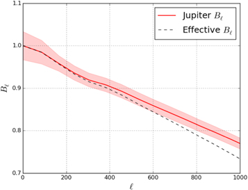
Figure 2. Reconstructed beam window function from Jupiter observations. Statistical error in the pointing model adds additional suppression of power at high ℓ, as indicated by the dashed effective beam curve. Shaded area represents the statistical error in the Jupiter beam window function.
Download figure:
Standard image High-resolution imageWe find a beam window function that is similar to, but marginally wider than, PB17 with a median Gaussian 36 full width at half maximum. This difference may be due to the telescope being imperfectly focused because the addition of the sapphire HWP lengthens the optical path between the primary and the secondary mirrors, or it may be due to diffraction off the HWP structure itself. We see no weather dependence or variation between seasons in the fitted beamwidth.
Boresight and detector statistical pointing error adds an additional suppression of high-ℓ power in the maps. The pointing model predicts residual pointing errors of 50'' rms. In Section 4.6, we fit an ℓ dependence to the overall gain amplitude, corresponding to the widening of the effective beam due to pointing error, and find no statistical preference for an additional widening of the effective beam due to pointing error. As a result, we convolve the beam function with a Gaussian corresponding to the best-fit pointing model error from the E-mode spectrum and include the effective beamwidth uncertainty in our multiplicative error estimate.
An additional source of systematic uncertainty in the beam comes from detector crosstalk. We measure the detector beam window function using temperature data but compute polarization power spectra. As described in Crowley et al. (2018), crosstalk acts differently in temperature, and polarization also acts differently in the presence of a continuous HWP, resulting in an effective beam mismatch. This effect is described in detail in Section 5.2. We find it to be subdominant to the statistical uncertainty for all spectra.
We estimate the polarization response to Jupiter and decompose this into scalar, dipole, and quadrupole terms. We subtract the scalar term as temperature-to-polarization leakage; this is described in Section 4.4. In Section 5.2, we show the contamination due to higher-order terms is negligible.
3.4. Detector Gains and Time Constants
Following PB14 and PB17, we use a three-step gain calibration to turn our TOD into physical temperature units with an additional correction for polarization efficiency. We measure a time-dependent gain calibration between detectors using a chopped thermal source before and after each set of four CESs. The gain is linearly interpolated between these measurements. We then calibrate these measurements to temperature on the sky using the same Jupiter scans conducted to measure the beam window function. Finally, we construct a CMB map and scale the overall amplitude of the polarization E-mode fluctuations to match the Planck 2018 data. Performing the absolute gain calibration with the E-mode spectrum jointly constrains the overall gain and polarization efficiency.
At several points during the observations, the thermal source used in the relative calibration was replaced for mechanical reasons. The conversion from the thermal source amplitude to temperature on the sky is performed separately for each source. PB14 describes a correction in this analysis due to the position of a cold HWP in the receiver. The cold HWP was stepped almost daily during the first half of the first season of observations, but it was never moved during the three seasons comprising this data set. We simulate the systematic error introduced by uncertainty on the measured gain acting on the CMB signal and find the contamination in all polarization spectra to be negligible. This is described in Section 5.2.
The detector time constants are measured by sweeping the frequency of the chopped thermal calibration source from 4 to 44 Hz. The source amplitude versus frequency is fit to a single pole transfer function. These time constants are interpolated linearly between the calibrations and deconvolved in the subsequent TOD processing.
3.5. Polarization Angle
The detector polarization angles and efficiencies are derived from dedicated raster scans of Tau A. The raster scan data is taken at 02 s−1 scan speed on the sky with the HWP rotating nominally. We deconvolve the detector time constants measured from a chopped thermal source calibration immediately before and after the Tau A raster scan. This is necessary because a phase lag between the detector TOD and the reconstructed HWP angle appears as a polarization angle error. After correcting for detector time constants, we find no significant correlation between the measured polarization angle and the precipitable water vapor (PWV) measured at the nearby Atacama Pathfinder Experiment41
(APEX) site. Without time-constant deconvolution, such a correlation is produced by the dependence of the time constants on the atmospheric loading and therefore the local PWV. The demodulated polarization TOD described in Section 4.1 is fit to a beam-convolved polarization map of Tau A from a measurement taken with the IRAM 30 m telescope (Aumont et al. 2010). We find statistically consistent detector polarization angles in focal plane coordinates compared to PB17 and no significant variation between seasons. We find the difference in measured polarization angle between detectors in a pair to be 905 ± 12. This is consistent with the design value of 90°. In Section 5.2, we simulate the expected systematic contamination due to detector polarization angle uncertainty at this level and find the effect to be negligible.
The measured polarized flux from these scans is used to estimate the polarization efficiency of the telescope and receiver. The polarization efficiency is degraded in three ways in addition to the non-ideality of the cold HWP described in PB14 and PB17.
These three effects are the non-ideality of the rotating HWP, the breaking of the Mizuguchi–Dragone (MD) condition (Mizugutch et al. 1976; Dragone 1978), and nonzero bolometer time constants. The modulation efficiency of the warm HWP is estimated from coherent source lab measurements and design detector bandpasses (Arnold et al. 2012). The polarization efficiency term due to the MD breaking is estimated from a GRASP42 physical optics simulation (Matsuda et al. 2018). The detector time constant acts as a time domain low-pass filter on the TOD, which has a response less than unity at the polarization modulation frequency. We find the measured values from the Tau A calibration to be consistent with the predictions—but with a larger statistical error, as expected. The non-ideality of the rotating HWP, cold HWP, and MD breaking polarization efficiency terms are intrinsic to the detectors and telescope geometry, and are corrected by rescaling the TOD and noise weights with the predicted values. The average contributions to the overall polarization efficiency from the rotating HWP, cold HWP, and MD breaking are ε ≈ 0.98, 0.98, and 0.93, respectively. The polarization efficiency due to the detector time constant depends on the numerical value of the time constant, which in turn depends on the detector bias point and optical loading. As a result, this polarization efficiency term is corrected by deconvolving the measured time constant from the chopped thermal source before and after each set of four CESs. The average polarization efficiency contribution from the detector time constants is ε ≈ 0.98.
We self-calibrate the overall polarization angle by fitting  following Keating et al. (2013). The overall polarization efficiency is degenerate with the absolute gain of the polarization maps and is set by matching the Polarbear E-mode spectrum to the Planck 143 GHz E-mode data on our patch. This is described in more detail in Section 4.6.
4. Data Analysis
In this section, we describe the formalism and processing steps used to turn the raw bolometer TOD into cosmological power spectra. We pay particular attention to ways in which the pipeline differs from PB14 and PB17.
4.1. TOD Processing
This analysis uses a pre-processing and demodulation procedure similar to that in T17 and Takakura et al. (2019), hereafter T19. A brief overview is provided here for completeness. For simplicity, terms relating to detector nonlinearity and instrumental polarization are neglected here. The raw bolometer TOD in the telescope frame can be modeled following
where χ ≈ ωt is the HWP angle, e−i4χ ≡ m(χ) describes the polarization modulation of the HWP, ε is a polarization efficiency, θdet is the detector angle with respect to instrument coordinates,  is the detector white noise, and A(χ, t) is a slowly varying HWP-synchronous structure in the TOD.
Prior to demodulation, we subtract the HWP-synchronous structure A(χ, t) using an iterative method similar to Johnson et al. (2007). The HWP angle is reconstructed from the encoder. The HWP synchronous structure is estimated following Kusaka et al. (2014) and is decomposed into harmonics. Gaps in the TOD are filled with the HWP synchronous structure. At each harmonic n ∈ {1, 2, ... 7}, the TOD are bandpass filtered with a bandwidth of 1 Hz and demodulated to form a time-dependent amplitude for that harmonic of the HWP synchronous structure. A linear drift is fit to the amplitude of each harmonic. The sum over n of these templates is subtracted from each TOD, and the process is iterated again. After the HWP structure has been subtracted, the polarization signal is reconstructed by multiplying the data by twice the conjugate of the modulation function 2m*(χ) and low-pass filtering to recover the polarization signal,

The TOD sampled at 8 Hz are used as the input to all subsequent analysis pipeline steps. Due to the high sample rate of the raw TOD and the number of Fourier Transform operations, including the demodulation in our main simulations would be computationally prohibitive. The window function associated with the 8 Hz sample rate is negligible for our ℓ range. The detector time constant deconvolution is performed on the demodulated polarization TOD.
Note that the noise in the demodulated TOD  is complex and both the real and imaginary components have twice the variance of the modulated detector white noise
  due to the factor of two necessary to recover Q and U correctly. There is no intrinsic difference in the polarization sensitivity compared to the pair differencing case. The noise
  can be well-described as white noise plus a single low-frequency component common to all detectors; this is described in Section 4.3. The demodulation algorithm assumes perfect separation of intensity and polarization signals in time domain frequency—in other words, the HWP frequency is much higher than the scan speed divided by the beam size. In Section 5.2, we quantify the impact of imperfect separation in the real data and find the effect to be negligible. These demodulated data are used as the input to the subsequent data characterization and mapmaking pipelines.
We record the low-pass filtered HWP structure subtracted TOD (the 0f or intensity component) and the demodulation at twice the HWP frequency (the 2f component) for data characterization and selection.
4.2. Data Characterization and Selection
The data selection framework used in this analysis consists of several rounds of increasingly selective criteria to characterize low-frequency noise and mitigate possible systematic contamination. The stages can be roughly described as cutting out glitches and effects well-localized in time, cutting data based on individual detector noise properties over the course of an observation, cutting data based on array noise properties, and cutting data based on map domain noise.
In all stages, the fundamental unit of data considered is the detector subscan. Data where the telescope is accelerating (turnarounds) are rejected completely. A table of efficiencies is shown in Table 2. The primary contributions to the end-to-end efficiency are the fraction of time the patch is available for observations, instrument downtime due to maintenance and weather, and overall focal plane yield due to nonfunctioning detectors and glitch cuts. A total of 2985 CES observations are used in the final mapmaking from the full observation period from 2014 July 25 until 2016 December 30.
Table 2. Operations and Data Selection Efficiency
| Category | Stage of Data Selection | Efficiency |
|---|---|---|
| Operations | Time spent observing patch | 36.8% |
| and yield | Focal plane yield | 50.7% |
| Data | Glitch cuts and off bolometers | 29.2% |
| Selection | Individual bolometer PSDs | 76.6% |
| Common mode PSD and maps | 79.6% | |
| Cumulative data selection | 17.8% | |
Notes. Data selection efficiency for this analysis. A total of 2985 hr long CESs have any data used in the final science analysis. The focal plane yield is normalized to the nominal number of optical bolometers, 1274. The cumulative data selection efficiency is the product of the preceding three rows.
Download table as: ASCIITypeset image
In the first stage, a set of time domain glitch criteria similar to those used in PB14 are applied to the pre-demodulated timestreams in order to find and remove high-frequency features. The TOD are convolved with a kernel designed to pick up sharp temporal spikes in the data while nulling the HWP synchronous structure at multiples of 2 Hz. Subscans where the maximum deviation of the convolved TOD is greater than ten times the standard deviation are discarded. This operation is performed on the full sample rate data to improve sensitivity to fast glitches. The post-demodulation intensity, 2f, and polarization TOD are convolved with an additional series of kernels sensitive to fast glitches in the TOD, and subscans are cut following the same criteria.
After these flagging steps, an analysis is performed to remove the low-frequency array common mode glitches in the polarization data that were shown in T19 to be correlated with polarized emission from clouds. We begin by performing a principal component analysis (PCA) on the detector intensity TOD. Working detectors are selected by removing channels whose intensity timestreams are not dominated by the largest eigenmode of the detector covariance matrix, due to atmospheric fluctuations. The Q + iU timestreams from each detector are rotated into the instrument frame via multiplication with  . These TOD are coadded to form a full focal plane common mode signal that is rotated again into minimum and maximum variance eigenmodes of the Q × U covariance matrix. Subscans where the ratio of the standard deviations of the two modes is greater than ten are cut. This corresponds to the TOD cloud detection criteria used in T19.
At this stage channels that have low signal-to-noise or bad fits to the chopped thermal calibration source, channels that have no position as measured by the beam calibration, and channels with no polarization angle measured from Tau A are cut.
In the second stage, each demodulated timestream is processed through the first portion of the mapmaking TOD filters described in Section 4.4. The TOD are filtered by a first-order subscan polynomial, ground-fixed structure is subtracted by binning the TOD in azimuth and subtracting the resulting template, and monopole temperature-to-polarization leakage is removed. Turnarounds and subscans flagged by the glitch cuts are filled in with white noise matched to the rms of the surrounding samples. The power spectral density (PSD) of the TOD is then measured and fit to a model consisting of white noise and a 1/f2 low-frequency noise term. Detectors with anomalously high white noise floors, high low-frequency noise, or poor fits to the model are discarded. For most individual bolometers, the low-frequency noise is undetectably small after the subscan polynomial filter. The action of the high-pass subscan polynomial filter imposes a floor of several times the scan frequency fscan ≈ 10 mHz on the knee frequency that can be resolved. Fourier domain lines in the PSD are noted and notched out in subsequent data processing. This notch filter is described in Section 4.4.
In the third stage, the common mode timestream is recomputed using the inverse variance individual detector weights, the additional data cuts, and Fourier notch filters defined in the previous stage. We fit the common mode PSD to a white noise and 1/fα term for instrument frame Q and U separately. White noise is largely uncorrelated between bolometers, whereas the low-frequency component is coherent across detectors—meaning that averaging detectors results in a higher knee frequency. The power-law index α is allowed to float because the higher knee frequency provides a sufficient lever arm to resolve the low-frequency exponent. Observations where the common mode knee frequency fknee in telescope frame Q (U) is greater than 150 mHz (100 mHz) or where the common mode noise floor is anomalously high are rejected. We find median knee frequencies of 45 mHz (24 mHz) in the common mode Q (U) PSDs and a median polarization white noise floor of  for Q and U individually in CMB temperature units. This corresponds to an array noise equivalent temperature of
  , which is comparable to PB14 and PB17. The knee frequency distributions differ because common mode Q and U noise are produced by different physical mechanisms. The Q low-frequency noise can be produced by temperature noise brought into the polarization TOD by temperature-to-polarization leakage subtraction or by spurious gain drifts acting on the HWP 4f structure. In contrast, U is out of phase with the 4f HWP structure and is approximately out of phase with the temperature-to-polarization leakage, meaning that low-frequency noise requires a phase drift of the HWP structure in the TOD produced by effects such as detector time constant drift. It is worth noting that we do not see a correlation between the array knee frequencies and the amplitude of the atmospheric fluctuations in the temperature data.
In the fourth stage, the detector weights computed in the second stage and the common mode PSD defined in the third stage are used to create individual observation maps, following the standard TOD filtering outlined in Section 4.4, with the modification that the telescope frame polarization is treated as a scalar field and is not rotated into R.A. and decl. coordinates. The maps are downsampled to degree pixels and a map χ2 is computed by comparing the fluctuation in the data to the expectation from the detector noise weights. Maps with an anomalously high χ2 are rejected as a check for low-frequency pathologies that are not readily visible in the common mode PSDs. In practice, this cut strongly overlaps with the common mode PSD criteria.
4.3. Low-frequency Noise Model
We define two noise models for use in our simulation pipeline, and show good overall agreement between the two. The noise in the data at low frequencies in the time domain can be described by a single common mode 1/fα component, meaning higher-order modes in the TOD covariance are negligible. We run the end-to-end analysis pipeline in two configurations: one using a TOD noise model and the other using random sign coaddition of individual CES maps to generate matched "signflip" noise realizations.
In the TOD noise model, we generate white noise on a per-detector basis, assuming no correlations between bolometers and the noise weights derived in Section 4.2. The common mode low-frequency noise is synthesized in telescope coordinates for Q and U separately, and is matched to the amplitude and power-law index α fit from the real data. This mode is then rotated into the polarization angle of each detector and added to the uncorrelated white noise.
In the "signflip" configuration, the noise realizations are generated by randomly assigning a + 1 or −1 factor to each map during the coaddition of CESs. This creates noise realizations with the exact power spectrum and correlation structure of the real data, assuming that the noise fluctuations between CESs are uncorrelated. This assumption can be broken by coherent drift in the amplitude of the ground synchronous structure, as described in Section 5.2. We find this effect to be negligible.
We find good agreement between the "signflip" noise realizations and the TOD noise realizations using our cross-spectrum estimator described in Section 4.5. The noise bias derived from both pipelines is shown in Figure 3. The full coadd and all null test splits described in Section 5.1 agree well, except for one null spectrum. In the "top versus bottom bolometers" case that explicitly splits paired detectors, we observe excess variance and an anticorrelation in map space between the two halves that cannot be reproduced by the simple TOD noise model. Temperature noise aliasing into the polarization frequencies in the TOD can create a similar noise anticorrelation. This is naturally accounted for in the "signflip" noise realizations.
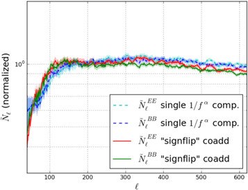
Figure 3. Noise bias comparison for the full data set from the TOD noise model and the signflip coaddition pipeline. We see broadly consistent results between the two noise models. Fiducial power spectra use the "signflip" noise model. These spectra do not reflect the filter transfer function and beam window function correction described in Section 4.5. "Signflip" curves with these corrections are shown in Figure 6. Shaded region represents the standard deviation of the simulated noise bias.
Download figure:
Standard image High-resolution imageWe use the random sign coaddition pipeline to generate the noise realizations used in our fiducial null tests and error bar estimation.
4.4. Mapmaking
In this analysis, we use a MASTER "filter and bin" mapmaker (Hivon et al. 2002) where the TOD is filtered to suppress low-frequency noise and projected onto the sky using inverse-variance noise weights.
The mapmaking pipeline takes the demodulated data described in Section 4.1 and applies an additional stack of time domain filters. The ordering of the filtering is set to avoid bias in the fitted temperature leakage coefficients by spurious modes in the temperature and polarization TOD.
The first filtering operation works in the Fourier domain and low-pass filters signal above 1.2 Hz. A set of notch filters are applied to Fourier domain glitches flagged in the data selection pipeline. A notch width of 10 mHz is used on every bolometer on the focal plane when a high-significance glitch is seen in more than 50 detectors for a given CES. An identical set of notch filters are applied to the simulation data.
The second filtering operation removes a second-order polynomial from each bolometer TOD for the whole CES. This mode is expected to be dominated by thermal fluctuations of the focal plane and cryogenics.
The third filter subtracts a ground-fixed template in I, Q, and U. The filter is constructed by averaging the telescope frame TOD in 144 azimuth bins and subtracting the resulting template from the TOD. This operation is performed independently for each bolometer and CES. Unlike PB14 and PB17, the same template is used for both left-going and right-going subscans. We expect that the ground synchronous structure in our data is due to telescope sidelobes far from the main beam interacting with the surrounding terrain. We conservatively assume no correlation between CESs, and subtract a unique ground-fixed template for each CES even though the ground fixed signal that we observe is generally stable between CESs. In Section 5.2, we place an upper limit on the error introduced by possible time variability in the ground-synchronous structure within each CES. We test varying the bin size and subtracting out a smoothed version of the template, and find no significant difference in the final measured power spectrum.
Once these modes have been projected out of the data, we perform a PCA similar to that in T17 to remove temperature-to-polarization leakage due to detector nonlinearity and instrumental polarization from the off-axis telescope design. We see a weak frequency dependence in the temperature leakage coefficients below the telescope scan frequency, and Fourier domain glitches in the TOD at high frequencies. As a result, to estimate the leakage coefficients, we form a copy of the TOD, apply a low-pass filter at 400 mHz, and subtract a first-order polynomial from each subscan. We then compute a 3 × 3 covariance matrix between the I, Q, and U TOD and average this between subscans. The leakage coefficients are determined using the PCA described in T17 with this covariance matrix. We find the estimated leakage coefficients to be stable over the course of our observations. The temperature leakage is subtracted from the original polarization TOD without the subscan polynomial and low-pass filters. Since the leakage coefficient determination is heavily dominated by atmospheric fluctuations, we do not expect this process to be significantly biased by cosmological signal. In Section 5.2, we simulate the error expected in the B-mode power spectrum due to multiplicative detector nonlinearity and find the effect to be negligible. We do not include this leakage or the PCA filter in our main simulation pipeline.
Following this, a first-order polynomial is subtracted from the Q and U TOD for each subscan in polarization to mitigate low-frequency noise. No further processing is applied to the I TOD, as these data are not used in the subsequent analyses.
Finally, a filter is applied to the data to suppress the low-frequency mode seen in all detectors. A low-pass filtered version of the Q and U array common mode is subtracted from each bolometer TOD in the instrument frame. The spectral shape of the low-pass filter is the inverse of the fit PSD of the stacked timestream derived in the data selection pipeline. The same filter is applied to simulated data. As described in Section 4.3, we do not see significant low-frequency noise beyond a single focal plane common mode.
We project the TOD into 8' pixels on the sky using a Lambert Cylindrical equal area projection. The resulting maps for the real data and a sample noise realization are shown in Figure 4. We achieve an effective map depth of 32 μK arcmin after correcting for the beam and TOD filtering.

Figure 4. PolarbearQ and U maps (top) and a sample noise realization (bottom) produced using the "signflip" coadd pipeline. CMB E-mode signal is visible in the real maps as a checkerboard pattern in Q and U. These noise realizations are used to estimate the band power covariance of the final power spectrum and the noise bias used in the foreground estimation pipeline.
Download figure:
Standard image High-resolution image4.5. Power Spectrum Estimation
The power spectrum estimation pipeline closely follows PB14 and "Pipeline A" in PB17, with several minor changes to improve numerical accuracy at low ℓ. A brief overview is provided for completeness.
The data set is grouped into 38 bundles of approximately uniform weight and sky coverage. We form power pseudo-spectra by taking cross-spectra between these bundles to remove the noise bias,

where  and w are the apodized Fourier transform and weight of each map bundle, respectively. The pseudo-spectrum is averaged into bins of Δℓ = 2. Following PB14, we use a pure B-mode estimator based on Smith (2006) and Smith & Zaldarriaga (2007). The apodization mask used in the pseudo-spectrum is significantly more aggressively smoothed than PB17. We apply an 8° cosine square edge taper and an 8° Hamming window to the pixel weight map. This improves the numerical stability of the reconstructed power spectrum at ℓ ≤ 100. We do not mask point sources in the power spectrum estimation. As described in Section 6.4, we do not see evidence for bright polarized point sources in higher-resolution versions of our maps, and we expect the contamination from unresolved polarized point sources to be negligible for this ℓ range.
The noise pseudo-spectrum  is taken to be the pseudo-spectrum of the sum of the apodized map bundles minus the cross pseudo-spectrum
  .
.
The pseudo-spectrum is taken to be a linear function of the true underlying power spectrum on the sky

where the transformation is given by

The mode-mixing matrix  describes the mixing of ℓ modes due to finite sky coverage and is estimated directly by computing the pseudo-spectrum of narrowband noise realizations. Here, Bℓ is the beam window function defined in Section 3.3. The filter transfer function is found via an iterative procedure, following PB14:
In contrast to PB17, we cut the iterative series off at n = 3 to avoid overfitting fluctuations in the simulated pseudo-spectra. This results in a negligible bias on the reconstructed power spectrum. The filter transfer function is calculated using simulated ΛCDM EE-only and BB-only skies drawn from the Planck 2018 baseline TT, EE, TE + lowE + lensing ΛCDM cosmology (Planck Collaboration et al. 2018b) with 1' pixels. We verify that the numerical value of the filter transfer function does not depend on the underlying cosmology used in the simulations.
We estimate the power spectrum in coarser bins of width Δℓ = 50. The binned estimate for the true power spectrum can be written using binning and interpolation operators  and
and  ,
,


The dependence of the binned spectrum on the underlying spectrum is given by the band power window functions  ,
,


These band power window functions are shown in Figure 5. The shape of the lowest bandpower is due to sensitivity degradation at low ℓ.

Figure 5. BB band power window functions. Shape of the lowest bandpower is due to the sensitivity degradation at low ℓ due to timestream filtering.
Download figure:
Standard image High-resolution imageWe have checked that the flat-sky approximation does not introduce a significant bias in the measured power spectra.
The statistical uncertainty on the reconstructed power spectrum is taken to be the standard deviation of the reconstructed power spectrum of Monte Carlo (MC) simulations containing filtered ΛCDM sky realizations and "signflip" noise realizations. We compute analytic uncertainties in the same way as PB14, and find those results to be consistent with our MC uncertainties.
For all spectra, we follow the Dℓ ≡ ℓ(ℓ + 1) Cℓ/(2π) convention unless otherwise noted.
4.5.1. E-mode and B-mode Mixing
The timestream filtering mixes E-mode power into the B-mode spectrum. This is subtracted in the pseudo-spectra following PB14,
This reconstructs the correct central value of  ; however, it does not remove the excess variance in the B-mode spectrum. We find that the level of B-mode power introduced by timestream filtering is comparable to the expected lensing B-mode signal in our lowest band power. Because the fluctuations due to leaked E-modes are below the fluctuations of the noise bias, the contribution to the statistical uncertainties is small. We nonetheless account for this effect in our statistical uncertainty by subtracting the measured E-mode spectrum in each realization in our simulations. We do not perform any matrix-based separation of E- and B-modes as described in BICEP2 Collaboration et al. (2016).
4.5.2. Quantifying Low-ℓ Statistical Performance
To accurately describe the low-ℓ statistical performance of Polarbear, it is necessary to account for the effect of the TOD filtering and the beam window function in the measured noise bias. We do this following BK15 by referring the noise pseudo-spectrum  to a true power spectrum on the sky Nb following Equation (7). We write the number of degrees of freedom per band power as an ℓ-dependent effective sky area. These two quantities represent the noise contribution to the power spectrum statistical uncertainties. Figure 6 and Table 3 show the results of this analysis. It should be noted that this is not exactly equivalent to an analytic estimate of the statistical errors, because it does not account for terms arising from the CMB signal variance.
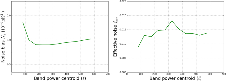
Figure 6. Noise bias Nb after correcting for TOD filtering and the beam window function (left), as well as the effective number of degrees of freedom νb per band power defined in Equation (19) written as an ℓ-dependent fsky = νb/(2ℓ · Δℓ), where ℓ and Δℓ refer to the nominal band power definitions (right). Degradation in Nb at high ℓ is primarily due to the beam window function, and degradation at low ℓ is due to low-frequency noise and timestream filtering. These curves are derived from the autospectrum of the "signflip" noise realizations computed using the fiducial cross-spectrum pipeline. The alternate autospectrum estimate described in Appendix gives similar Nb with a marginally larger effective fsky. This plot can be directly compared to Figure 3 in BK15. Numerical values for these curves are given in Table 3.
Download figure:
Standard image High-resolution imageTable 3. Noise Bias and Effective Degrees of Freedom
| Nominal Band Definition (ℓ) | Band Power Centroid (ℓ) | Noise Bias Nb (10−4 μK2) | Effective Noise (fsky) |
|---|---|---|---|
| 50 < ℓ ≤ 100 | 81.5 | 1.665 | 0.0089 |
| 100 < ℓ ≤ 150 | 125.6 | 1.006 | 0.0130 |
| 150 < ℓ ≤ 200 | 175.1 | 0.875 | 0.0125 |
| 200 < ℓ ≤ 250 | 224.8 | 0.872 | 0.0147 |
| 250 < ℓ ≤ 300 | 274.4 | 0.872 | 0.0149 |
| 300 < ℓ ≤ 350 | 324.8 | 0.891 | 0.0181 |
| 350 < ℓ ≤ 400 | 374.9 | 0.921 | 0.0152 |
| 400 < ℓ ≤ 450 | 425.0 | 0.943 | 0.0136 |
| 450 < ℓ ≤ 500 | 474.8 | 0.963 | 0.0137 |
| 500 < ℓ ≤ 550 | 524.7 | 0.998 | 0.0130 |
| 550 < ℓ ≤ 600 | 574.7 | 1.030 | 0.0137 |
Note. Data points for the curves shown in Figure 6. These data use the "signflip" noise model and the fiducial internal cross power spectrum estimator. These numbers are written in Cℓ units and do not include the factor of ℓ(ℓ + 1)/2π used in the rest of this work.
Download table as: ASCIITypeset image
We additionally compute an ℓ knee that can be compared to the numbers presented in The Simons Observatory Collaboration et al. (2019). We fit our estimated power spectrum uncertainties following the same formalism and find a knee of ℓ = 90. This ℓ knee can also be computed by incorporating the effective sky area degradation into the noise bias,  , using the numbers in Table 3 giving consistent results.
4.6. Map Level Calibration
We perform an overall gain calibration by cross-correlating our data to the Planck satellite. We use the Planck 2018 PR3 143 GHz full mission maps43 and process them through our filtering and mapmaking pipeline. We compute debiased spectra for both the Polarbear internal cross-spectra using the fiducial power spectrum estimate and the fully coadded Polarbear maps correlated with the scanned Planck maps using the full coadd power spectrum estimator described in Appendix. We fit an overall gain calibration factor based on the ratio of the E-mode spectra,

The uncertainty on this ratio is computed via MC simulation, holding the underlying sky realization fixed. We use 96 realizations of the Planck FFP10 noise model (Planck Collaboration et al. 2018a) to approximate the Planck map noise. We fit this calibration to an ℓ-dependent gain model, accounting for a smearing of the beam profile following:


We find an overall gain calibration factor of 1.08 ± 0.04 in amplitude and an effective beam smearing of σ2 = 1.14 ± 5.58 arcmin2. We convolve the beam with the best-fit value for the pointing model error and treat the uncertainties in g0 and σ2 as a calibration error term in our final results. We compute an alternate absolute gain calibration fitting the Polarbear spectrum to the best-fit Planck ΛCDM theory spectrum and find agreement with the fiducial calibration at the percent level across our ℓ range.
After applying this absolute calibration, we compare the E-mode spectrum to Planck and form a null spectrum:

The uncertainty on this null spectrum is computed via MC. We find this null spectrum to be consistent with zero with χ2/ν = 7.0/9, corresponding to a probability to exceed (PTE) of 64%. When we compare our measured E-mode spectrum to the best-fit ΛCDM theory, we observe a marginally significant discrepancy in our highest two ℓ bins. This appears to be due to an anisotropic feature seen in the two-dimensional power spectrum at approximately the size scale and orientation of the detector wafers. These fluctuations have no significant counterpart in the null tests described in Section 5.1. These fluctuations do not depend on any of the operations in the TOD filtering and mapmaking pipeline that have characteristic scales on the sky or frequencies in the time domain. The overall gain and beam calibration does not significantly shift if these two bins are removed from the analysis. We find that there is no significant shift in the B-mode spectrum when these regions of the Fourier plane are masked in the pseudo-spectrum estimation. We show our measured E-mode spectrum as well as the residuals compared to Planck and the ΛCDM theory in Figure 7.
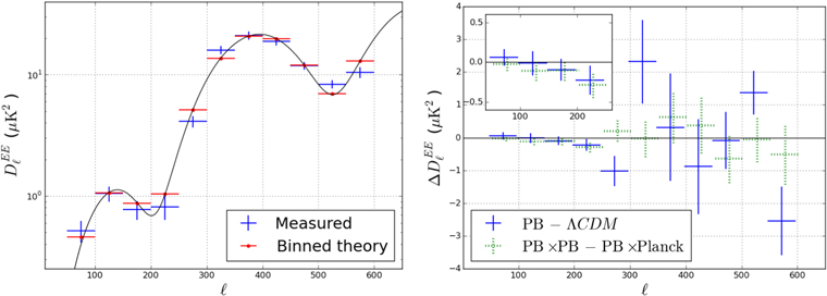
Figure 7. The E-mode band powers after absolute gain calibration compared to the best-fit Planck 2018 ΛCDM cosmology (left), and the residuals compared to the binned theory and the null quantity formed by subtracting the debiased cross-spectrum with filtered Planck 2018 143 GHz maps (right). The E-mode spectrum is used as an overall gain and effective beamwidth calibration. The lowest four bandpowers are shown in the inset.
Download figure:
Standard image High-resolution imageAfter applying the overall gain calibration, we self-calibrate the overall instrument polarization angle following Keating et al. (2013). We apply an overall polarization angle correction Δψ, such that the measured  power is minimized:
Here,  is the uncertainty in the reconstructed EB spectrum from the MC simulations. We find an overall calibration Δψ = −061 ± 022. After applying this calibration, we find that
  is consistent with zero, with a total χ2 PTE of 77%. Our absolute angle calibration is compatible with PB17, which reported Δψ PB17 = −079 ± 016. This calibration is shown in Figure 8. It should be noted that this calibration is independent of PB17.
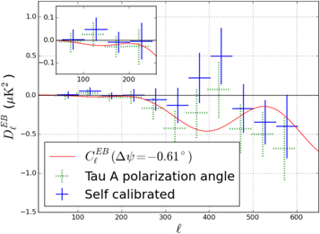
Figure 8. EB power spectrum based on the IRAM Tau A measurement, after polarization angle self-calibration. We find the angle derived from self-calibration to be statistically consistent with PB17. We find our measured EB spectrum to be consistent with zero after an overall polarization angle is subtracted, with χ2/ν = 6.56/10 corresponding to a 77% PTE. The lowest four bandpowers are shown in the inset.
Download figure:
Standard image High-resolution imageThe self-calibrated polarization angle correction is applied in the map domain. The absolute gain computed with the EE spectrum differs slightly from the MC simulations used to establish the band power errors and covariances. To account for this in the final power spectrum uncertainties, we assume that the total variance in each band power is the sum of the signal variance and the noise variance as derived from signal-only and noise-only simulations, respectively. The noise variance is rescaled to the best-fit absolute gain calibration.
We quantify a calibration uncertainty in the measured power spectrum using the uncertainty in the overall gain calibration g0, pointing model error σ2, polarization angle self calibration Δψ, and statistical uncertainty on the beam window function ΔBℓ. The correlation between g0 and σ2 is modeled as a simple Gaussian covariance. The three effects are added in quadrature to form a total calibration error. This represents an upper limit, as the overall gain calibration and beam window function are degenerate. The numerical values of these calibration errors in the estimated power spectrum are shown in Section 6.1.
5. Systematic Uncertainties
In this section, we describe the internal consistency checks performed with the data and simulation of known systematic contaminants.
5.1. Null Tests
We perform a set of null tests to establish the internal consistency of the data set and search for possible systematic contamination in the final power spectra. In general, it is not possible to construct difference maps between halves of the data with zero signal due to anisotropic scanning and filtering effects. This effect becomes particularly pronounced at low ℓ. As a result, we follow the formalism developed originally by the QUIET collaboration (Bischoff 2010) and used in PB14 and PB17. We include the filtering and mode mixing explicitly in the construction of the null spectrum

where  and
and  are the debiased autospectrum for each half of the split. Likewise,
  is the cross-spectrum between the splits. The spectra are computed using the same cross-spectrum formalism and map bundles used in the main pipeline.
The filter transfer function and mode-mixing matrix are computed in the same way as the fiducial power spectrum pipeline, using 92 EE-only and 92 BB-only Planck 2018 ΛCDM input maps for each test. Only map regions present in both halves of the split are used to form the pseudo-spectrum and mode-mixing matrix. The null spectra are computed using the same ℓ binning as the final power spectrum. The EE, EB, and BB null spectra are compared to 192 EE + BB signal and noise simulations. We find that this number of simulations is adequate for percent-level statistical uncertainties on the null spectrum PTE values and filter transfer functions across our full ℓ range.
For our fiducial null test statistics, we use noise realizations generated with the "signflip" pipeline. There is no significant difference from the PTE values computed with the TOD noise model, with the exception of the "top versus bottom" null test that explicitly separates detector pairs. This is due to the presence of an additional anticorrelated noise term when detector pairs are separated that is not included in the TOD noise model described in Section 4.3.
5.1.1. Null Test Data Splits
We split the data along 18 largely uncorrelated axes designed to probe a wide range of possible sources of systematic contamination. Where possible, the data set is split into halves with equal weight. In the following, we briefly describe these splits.
- 1."First half versus second half:" the data set is split chronologically into two equal-weight halves, to probe for time-dependent miscalibration or changes in the instrument.
- 2."Rising versus middle and setting," "middle versus rising and setting," "setting versus rising and middle:" the three different CES types are split in all possible combinations, to detect elevation-dependent miscalibration or residual ground-synchronous signal.
- 3."Left-going versus right-going subscans:" the data set is split in half according to the direction of motion of the telescope, to test for microphonic or magnetic pickup in the data.
- 4."High-gain versus low-gain observations:" the data set is split into observations with above- and below-average mean detector gain coefficients, to search for problems with the gain calibration.
- 5."High PWV versus low PWV:" the data set is split by PWV as measured by the nearby APEX radiometer, to check for loading- or weather-dependent effects.
- 6."Common mode Q knee frequency," common mode U knee frequency: the data set is split into observations with high and low knee frequencies in the telescope frame Q and U common mode signal, to check for problems in the treatment of low-frequency contamination. The Q knee frequency split overlaps with the cloud detection criteria from T19. Both splits are largely uncorrelated with the PWV split.
- 7."Mean temperature-to-polarization leakage by channel:" split the data set into detectors that see small and large temperature-to-polarization leakage coefficients, to test the subtraction and search for residual contamination.
- 8."2f amplitude by channel," "4f amplitude by channel:" split the data by HWP signal amplitude, to check for problems removing the HWP structure or systematic contamination coupling into the data through these terms.
- 9."Q versus U pixels:" each detector wafer is fabricated with two sets of polarization angles. We split the data into the two pixel types to check for problems in the device fabrication.
- 10."Sun above or below the horizon," "Moon above or below the horizon:" we split observations based on whether or not the Sun or Moon is up, to check for residual sidelobe contamination.
- 11."Top half versus bottom half," left half versus right half: we split detectors by the boresight axis of the telescope, to check for optical distortion and problems due to far sidelobes.
- 12."Top versus bottom bolometers:" with a continuous HWP, each bolometer TOD independently measures Q and U. We explicitly separate detector pairs in order to check for temperature aliasing or device mismatch.
We have also considered season-by-season data splits. These are not included in the final suite, however, because they are highly correlated with the first half versus second half split. Furthermore, we have examined average 2f and 4f amplitudes as well as average temperature-to-polarization leakage by observation, but exclude these due to redundancy with the weather and gain splits. We also considered Sun and Moon boresight distance splits, but exclude them due to overlap with the Sun and Moon being above the horizon. None of the excluded splits indicated significant problems in earlier iterations of the pipeline, and removing redundant tests improves sensitivity to outliers in the splits used.
5.1.2. Null Test Statistics and Analysis
For each bin in each null spectrum, we compute the statistic  , where
  is the standard deviation of the MC null spectra. We use both χnull and
  because the former is more sensitive to systematic biases and the latter is more sensitive to outliers. Figure 9 shows the χnull and
  distributions compared to the expectation from MC simulations. Table 4 shows the PTE of the total
  summed over ℓ bins for each test and summed over tests for each bin.
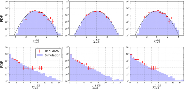
Figure 9. One-dimensional χnull = Cnull/σnull,MC distribution from the fiducial set of null test splits (top), and the same data shown as  (bottom). No statistically significant outliers are seen in these data. Error bars on the real data histograms represent 68% Poisson confidence intervals. Solid line in the upper panels shows a unit variance Gaussian as an approximation to the real distribution. Note that the summary statistics do not assume a Gaussian distribution for χnull, because the data are only compared to the simulations.
Download figure:
Standard image High-resolution imageTable 4. Null Test PTE Values
| Total EEχ2 PTE | Total EBχ2 PTE | Total BBχ2 PTE | |
|---|---|---|---|
| Null test summed over ℓ bins | |||
| First half versus second half | 86.5% | 43.2% | 79.7% |
| Rising versus middle and setting | 85.4% | 70.8% | 6.8% |
| Middle versus rising and setting | 63.0% | 63.0% | 39.1% |
| Setting versus rising and middle | 50.5% | 53.1% | 19.3% |
| Left-going versus right-going subscans | 36.5% | 26.0% | 6.2% |
| High-gain versus low-gain CESs | 45.3% | 83.3% | 3.1% |
| High PWV versus low PWV | 50.5% | 33.9% | 28.6% |
| Common mode Q knee frequency | 57.8% | 36.5% | 26.6% |
| Common mode U knee frequency | 91.7% | 54.7% | 79.7% |
| Mean temperature leakage by bolometer | 78.6% | 54.2% | 56.8% |
| 2f amplitude by bolometer | 5.7% | 32.8% | 83.9% |
| 4f amplitude by bolometer | 35.4% | 18.2% | 33.3% |
| Q versus U pixels | 72.4% | 64.6% | 28.1% |
| Sun above or below the horizon | 76.6% | 91.1% | 32.2% |
| Moon above or below the horizon | 76.0% | 77.6% | 57.3% |
| Top half versus bottom half | 79.7% | 35.4% | 27.1% |
| Left half versus right half | 53.6% | 33.9% | 76.0% |
| Top versus bottom bolometers | 36.5% | 55.7% | 35.4% |
| ℓ bin summed over null tests | |||
| 50 ≤ ℓ ≤ 100 | 31.8% | 58.3% | 44.8% |
| 100 < ℓ ≤ 150 | 64.1% | 14.1% | 24.5% |
| 150 < ℓ ≤ 200 | 61.5% | 46.9% | 96.9% |
| 200 < ℓ ≤ 250 | 71.4% | 74.0% | 28.6% |
| 250 < ℓ ≤ 300 | 83.9% | 7.3% | 26.6% |
| 300 < ℓ ≤ 350 | 50.5% | 92.7% | 6.8% |
| 350 < ℓ ≤ 400 | 64.1% | 97.9% | 92.2% |
| 400 < ℓ ≤ 450 | 44.3% | 84.4% | 5.2% |
| 450 < ℓ ≤ 500 | 96.9% | 63.5% | 3.1% |
| 500 < ℓ ≤ 550 | 68.8% | 84.5% | 49.0% |
| 550 < ℓ ≤ 600 | 49.5% | 16.1% | 49.5% |
Note. PTE values for the total χ2 of each null spectrum summed over ℓ bins and each ℓ bin summed over null spectra. None of the null spectra indicate significant problems. PTE values are computed directly from the 192 signal+noise simulations and are therefore quantized at the 0.5% level.
Download table as: ASCIITypeset image
To probe for systematic contamination and consistency of the noise model, we compute five statistics on the χnull values. These statistics were determined before computing spectra with the real data.
- 1."Average χ overall:" the mean value of χnull for all tests and bins
- 2."Most extreme χ2 by bin:" the most extreme
 when summing spectra over tests
 - 3."Most extreme χ2 by test:" the most extreme when summing spectra over bins
- 4."Most extreme χ2 overall:" the most extreme for all bins and tests
- 5."Total χ2 overall:" the sum of for all spectra


For each statistic, we compute a PTE by comparing the real data to same statistic computed with the MC realizations. Directly comparing the data to the simulations accounts for any correlations that exist between bins and tests in the computation of the PTE values. We define an additional statistic Plow, which is the lowest of the five PTE values. We require that the PTE of Plow be greater than 5%. The numerical value for these statistics can be seen in Table 5. All spectra (EE, EB, and BB) pass these criteria.
Table 5. Null Test PTE Values
| Null Statistic | EE PTE | EB PTE | BB PTE |
|---|---|---|---|
| Average χ overall | 73.4% | 80.7% | 9.9% |
| Most extreme χ2 by bin | 96.9% | 43.8% | 31.7% |
| Most extreme χ2 by test | 70.3% | 98.4% | 57.3% |
| Most extreme χ2 overall | 48.4% | 84.9% | 66.1% |
| Total χ2 overall | 90.6% | 78.7% | 12.5% |
| Lowest statistic | 85.4% | 86.4% | 33.9% |
| KS test on all bins | 10.1% | 60.4% | 15.9% |
| KS test on all spectra | 6.4% | 31.8% | 10.5% |
| KS test overall | 35.9% | 27.5% | 14.6% |
Note. PTE values for each of the high-level null test statistics.
Download table as: ASCIITypeset image
In addition, we require that the PTE of the  values by test, by bin, and overall be consistent with a uniform distribution, using a Kolmogorov–Smirnov (KS) test to check for systematic mismatch between the real and simulated uncertainties. Figure 10 shows the PTE distribution for all bins and tests. We find the PTE distributions to be consistent with uniform.

Figure 10. Distribution of PTE values for each bin in each test. Distributions for all three spectra are consistent with uniform.
Download figure:
Standard image High-resolution image5.2. Simulation of Systematic Errors
In addition to the null tests, we simulate several known sources of systematic error. We find upper bounds on the contamination introduced by these effects to be subdominant to the statistical error in all spectra.
The systematic error estimate uses a modified version of the simulation pipeline developed for the null tests and the power spectrum estimation. For most systematic effects, a signal-only ΛCDM sky is scanned to form simulated TOD. Next, these TOD are distorted following a model of the given effect, and then filtered and projected onto the sky using the fiducial mapmaker. We compute pseudo-spectra from these distorted maps and refer them to the underlying sky using the same mode coupling and filter transfer functions used for the fiducial power spectrum estimate. Since several systematics are suppressed by the overall gain and polarization angle calibration, we perform these overall calibrations in each simulation. We do not model the ℓ-dependent gain model applied to the real data, and only fit the overall gain g0. In parallel, the same mapmaking and power spectrum estimation is performed without distorting the TOD to form a reference simulation. The systematic error is taken to be the absolute difference between the contaminated and reference power spectra.
To form an overall systematic error estimate, we linearly add the power spectrum contamination from each set of simulations. In practice, we expect that each source of error will be largely uncorrelated with the others, meaning this is a conservative upper limit. The total systematic error estimate as well as the contributions from groups of effects in EE and BB are shown in Figure 11. We find the expected systematic contamination in the EB spectrum to be likewise subdominant to our statistical errors.

Figure 11. Systematic contributions from all simulated effects, grouped thematically for EE and BB (left and right). Ground structure curve indicates the sum of contamination from the detector gain and linear drift models of ground contamination. HWPSS and aliasing curve includes 0f and 2f signal aliasing as well as the HWP imperfections. Polarization angle curve shows the sum of individual and overall polarization angle uncertainties after self-calibration. Beams and pointing curve includes pointing model uncertainty and effects related to detector crosstalk. Gain and nonlinearity curve includes relative gain uncertainty, as well as detector gain and time-constant drift acting on the CMB signal. The dominant effect in EE is the misestimation of the effective polarization beam due to detector crosstalk, while the dominant systematic in BB is the uncertainty in the ground structure subtraction. It should be noted that this is a conservative estimate driven by significant model uncertainties. Future experiments may be able to suppress this effect significantly through careful study and control of ground pickup. Total systematic error is formed assuming all systematics add linearly in power.
Download figure:
Standard image High-resolution image5.2.1. Gain Miscalibration, Time Constant Drift, Detector Nonlinearity
We simulate the error introduced by finite uncertainty on the relative gain calibration of each detector. We estimate the statistical uncertainty in each bolometer relative gain calibration to be 4.7%, due to the amplitude of the chopped thermal source and detector noise.
As described in T17, the primary impact of detector nonlinearity is the additive temperature-to-polarization leakage. However, there is a smaller multiplicative term from the gain variation acting on the CMB signal. We simulate this using a downsampled version of the normalized 4f amplitude (phase) as a tracer of the detector small signal gain (time constant), and inject the nonlinear response (time-dependent polarization angle error) into the simulation timestreams. The time-constant drift and detector nonlinearity modulating the ground-synchronous structure are modeled separately.
5.2.2. Polarization Angle Error
We estimate the impact on the reconstructed power spectrum assuming that the calibrated detector polarization angle errors are Gaussian distributed around the true values with standard deviation 12. This error estimate is taken from the scatter of the difference in polarization angles measured for the two detectors within a pair. This polarization angle uncertainty is comparable to the value used in PB17. The systematic effect is strongly suppressed by the absolute polarization angle calibration. We also estimate the effect of an overall polarization angle miscalibration by rotating the polarization angle of the input sky 05 rms based on the quoted systematic uncertainty in the Tau A polarization angle from Aumont et al. (2010). It should be noted that this measurement was performed at 90 GHz. Several other experiments (Naess et al. 2014; Planck Collaboration et al. 2016; Kusaka et al. 2018; Ritacco et al. 2018) have measured Tau A at 150 GHz and found consistent results. The residual error from an overall polarization angle shift is not identically zero after self-calibration, because the map-making operation is not invariant under polarization angle rotation, due to different Q and U common mode filtering.
5.2.3. Boresight Pointing Error
We quantify the systematic impact of the imperfect knowledge of the boresight pointing by considering several candidate pointing solutions. We perform the input map scanning with the fiducial pointing model and project the TOD to the sky with an alternate pointing solution derived using different subsets of the point-source observations or model parameters. We find the largest discrepancy from the fiducial pointing solution results from the inclusion of Jupiter data in the pointing model fit. We conservatively quote that residual in our systematic error estimate. This is one of the largest systematic uncertainties in our E-mode spectrum; however, this effect is significantly less than our statistical error over our ℓ range. This effect has a significantly smaller impact on the B-mode spectrum.
5.2.4. Crosstalk
We observe an electrical coupling between detector readouts on the same cables. We assume that this crosstalk is linear and constant through the entire data set. We estimate the amplitude of this effect using the observations of Jupiter used for the gain and beam calibration. Crosstalk appears in these data as an apparent negative copy of the beam shape several tens of arcminutes away from the main beam. We estimate the amplitude of these images using a matched filter and construct a matrix representing the coupling of signal in detector i to observed signal in detector j,

We find the matrix  to be sparse, and do not see significant crosstalk for detector readout on different cables. The median nonzero off-diagonal element of the matrix
  is 1%, and the median row sum representing the ratio of crosstalked power to power in the main beam is approximately 4%.
We estimate this systematic error as the sum of two effects. We first quantify error introduced in the beam calibration. This is due to the fact that crosstalk is strongly suppressed in polarization because of the different polarization angles of each detector (Crowley et al. 2018) in HWP experiments. As a result, the temperature and polarization see different effective beam profiles. The second effect is the direct distortion of the polarization signal, which we simulate by injecting crosstalk at the TOD level in signal-only simulations. We find the beam miscalibration effect to be the dominant systematic in our E-mode spectrum. It is possible to strongly suppress crosstalk by inverting the mixing matrix  in the data processing pipeline as done in Henning et al. (2018). We do not take this step, however, as the expected contamination is already below our statistical error.
5.2.5. Ground Pickup
We observe a ground-fixed structure in the TOD that is on the order of 100 μK after subscan polynomial filtering. The majority of the effect is subtracted by binning each detector TOD in azimuth and subtracting that mode for each CES. This structure is likely optical and due to far sidelobes sensing the surrounding terrain. We simulate possible variation in this ground-fixed structure within each CES, and estimate the impact of the residual on the final B-mode power spectrum. We find this to be the dominant source of possible systematic contamination in our lowest B-mode spectrum ℓ bin.
One physically motivated model for this effect is the detector nonlinearity modulating stable ground pickup. We simulate this using the low-pass filtered 4f amplitude as a gain tracer. As shown in T17, the dominant source of 4f amplitude variation is detector nonlinearity modulating the detector small signal gain. This gain function modulates the ground-fixed structure producing imperfect subtraction by the TOD filters.
In addition to the detector gain model, we simulate several linear drift models of instability in the ground template. We simulate the apparent ground structure amplitude drifting during the course of a CES, and place an upper limit on this model using the TOD directly. For each bolometer and CES type (rising, middle, and setting), we fit Q + iU for each subscan as a tenth-order Legendre polynomial series. We then average these coefficients across all CESs, to build a set of polarization templates for the ground synchronous structure. The TOD is then fit to this template for each subscan and averaged across detectors to fit a ground amplitude as a function of subscan number within an CES. The slope of this amplitude is then computed for each CES. We do not see any correlation of the ground amplitude or the slope of the amplitude with local solar or sidereal time, and place an upper limit of 1% temperature drift correlated between CESs. We simulate a ground-synchronous signal amplitude increase of 1% in each CES to place an approximate upper limit on the BB power created by this model.
We also expect that the ground-fixed signal amplitude drift within a CES will have a component uncorrelated with solar or sidereal time. We simulate this by assuming that all of the variance in the ground amplitude slope is due to physical temperature drift of the apparent ground-fixed signal. This model appears primarily as low-ℓ noise in the map domain. We quantify the estimated residual after suppression by the cross-spectrum estimator. It should be noted that this represents the maximum possible contamination for this model that is consistent with the data and receives some contribution from the TOD noise. The majority of the possible systematic contamination due to ground-fixed signal comes from this mode. The physically motivated gain modulation predicts a significantly smaller level of contamination.
We also validate that the null test statistics are sensitive to these models of drift in the observed ground structure amplitude. Statistically significant contamination due to imperfect ground template subtraction results in null test failures confined to the lowest ℓ bin of the CES type (rising, middle, setting) and half focal plane (left versus right and top versus bottom) splits. While less sensitive than the template approach, the null tests are significantly more model-independent, in that the contamination need not follow the linear drift or 4f gain models. Since no such failure is observed, we can be confident that this systematic error is indeed subdominant to our statistical errors.
5.2.6. HWP Signal Aliasing
An additional source of variance in the polarization data is produced by the imperfect separation of temperature and polarization in time domain frequency. While small, the (beam-convolved) temperature signal on the sky will have power that aliases into the polarization band centered at the HWP 4f. Furthermore, there is nonzero leakage of the temperature signal into the sidebands of the HWP 2f amplitude. We simulate these effects by scanning a temperature-only beam-convolved sky and injecting the aliased signal at the 0.6% level via the 2f and directly via the 0f into the polarization TOD. We find the contamination in both the E- and B-mode channels to be negligible. We do not simulate the impact of the TOD filtering on this systematic, and simply bin the pseudo-spectrum of the aliased maps.
5.2.7. HWP Imperfections
We observe a small air bubble in the antireflective coating on our warm HWP. We find the HWP synchronous structure associated with this spot to be stable with time. We simulate the aliased power from the total non-4f harmonics coupled with nonlinearity, time constant drift, and gain error and find the excess variance added to the data to be negligible.
5.2.8. Temperature-to-polarization Leakage
The temperature-to-polarization leakage produced by the off-axis telescope design has both scalar and higher-order terms. Following Essinger-Hileman et al. (2016), we break the leakage into scalar, dipole, and quadrupole terms. We measure the higher-order modes using the scans of Jupiter performed for the beam calibration. We find the contamination from these higher-order modes in the polarization power spectra to be negligible. More details on this analysis can be found in Takakura (2017).
5.2.9. Cross Polarization from MD Breaking
The systematic contamination due to cross polarization from the breaking of the MD condition by the HWP located at the focus of the primary is expected to be negligible. Matsuda et al. (2018) simulated the impact of this cross polarization for the Polarbear-2 receiver assuming the same observation strategy used in this analysis. Due to the focal plane dependence of the cross polarization and the smaller field of view of the Polarbear instrument, the contamination will be smaller than the expectation for Polarbear-2.
6. Power Spectra and Parameter Constraints
In this section, we present our power spectrum results, an estimate of the foreground contamination in our spectra, and an upper limit on the tensor-to-scalar ratio r.
6.1. Polarbear Power Spectrum

Our estimated B-mode power spectrum is shown in Figure 12. We observe a modest excess above the ΛCDM lensing expectation in our lowest two ℓ bins.
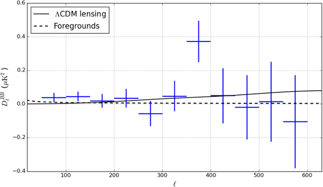
Figure 12. Measured B-mode spectrum using the fiducial cross-spectrum pipeline. Error bars shown reflect only the statistical uncertainties. Numerical bandpowers including systematic and calibration errors can be found in Table 6. Dashed foreground curve represents the best-fit dust power at 150 GHz described in Section 6.5. Outlier at ℓ = 375 has a PTE of 9% when the trials factor from the 11 bandpowers is taken into account; therefore, it is not statistically significant.
Download figure:
Standard image High-resolution imageThe band power uncertainties from all terms (statistical, systematic, and calibration) are shown in Table 6. We find the statistical error to be dominant in all ℓ bins.
Table 6. Band Powers and Uncertainties
| Nominal Band Definition |
 (μK2) (μK2) |
 stat error (μK2) stat error (μK2) |
 syst error (μK2) syst error (μK2) |
 cal error (μK2) cal error (μK2) |
|---|---|---|---|---|
| 50 < ℓ ≤ 100 | 0.0390 | 0.0268 | 0.0040 | 0.0027 |
| 100 < ℓ ≤ 150 | 0.0449 | 0.0288 | 0.0010 | 0.0023 |
| 150 < ℓ ≤ 200 | 0.0194 | 0.0415 | 0.0012 | 0.0009 |
| 200 < ℓ ≤ 250 | 0.0345 | 0.0559 | 0.0007 | 0.0014 |
| 250 < ℓ ≤ 300 | −0.0566 | 0.0747 | 0.0015 | 0.0019 |
| 300 < ℓ ≤ 350 | 0.0471 | 0.0910 | 0.0022 | 0.0019 |
| 350 < ℓ ≤ 400 | 0.3731 | 0.1236 | 0.0022 | 0.0168 |
| 400 < ℓ ≤ 450 | 0.0503 | 0.1641 | 0.0021 | 0.0031 |
| 450 < ℓ ≤ 500 | −0.0189 | 0.1907 | 0.0029 | 0.0017 |
| 500 < ℓ ≤ 550 | 0.0143 | 0.2377 | 0.0019 | 0.0015 |
| 550 < ℓ ≤ 600 | −0.1037 | 0.2765 | 0.0049 | 0.0126 |
Notes. Measured bandpowers as well as the statistical, combined systematic, and calibration uncertainty error estimates. The calibration and systematic error estimates are described in Sections 4.6 and 5.2, respectively.
Download table as: ASCIITypeset image
We compute an estimate of the overall amplitude of our observed B-mode signal relative to previous measurements. For the purposes of this calculation, we assume that the underlying sky consists of a lensing CMB component corresponding to the Planck 2018 ΛCDM lensing B-mode spectrum and a foreground component modeled by a power law  taken from the BK15 spectral decomposition at 150 GHz. We find a reduced χ2 of 11.6/11 compared to this model indicating good agreement. Naively fitting for an overall B-mode amplitude to rescale this template, we find ABB = 1.8 ± 0.8, disfavoring the null BB hypothesis at 2.2σ. This estimate neglects the slightly non-Gaussian shape of the band power distributions. However, that is accounted for in our cosmological parameter constraints, as shown in subsequent sections.
We additionally compute a naive uncertainty on r from our ΛCDM lensing-only (r = 0) simulations. We find σ(r) = 0.34, neglecting the non-Gaussian shape of the likelihood.
6.2. Cross-correlation with Planck HFI Maps
We compute cross-spectra with three Planck 2018 High Frequency Instrument (HFI) maps to quantify the contribution of galactic dust to our B-mode autospectrum. We form ten unique auto- and cross-spectra between four maps:
- 1.Polarbear 150 GHz map;
- 2.Planck 143 GHz frequency map;
- 3.Planck 217 GHz frequency map;
- 4.Planck 353 GHz frequency map.
We process the Planck PR3 full mission frequency maps through the Polarbear observing pipeline to create Planck maps as seen by Polarbear. Additionally, we process 96 noise realizations from the Planck FFP10 noise simulations for each frequency, to establish the Planck noise bias. The Polarbear noise bias is estimated using 192 "signflip" noise realizations.
The spectra involving the Planck maps are formed using the alternate full autospectrum pipeline described in the Appendix, where we simply compute the power spectrum of the fully coadded map rather than the cross-spectrum of the ten-day data subsets. We compute the measured debiased power spectrum  for display purposes by subtracting the mean autospectrum of the FFP10 noise simulations from the autospectrum of the real map. This is done to avoid relying on same-frequency cross-spectra in the Planck 2018 PR3 maps, which are known to be contaminated by systematics at the lowest ℓ values (Planck Collaboration et al. 2018a).
The Polarbear autospectrum and noise bias are computed using the fiducial cross-spectrum pipeline. Using the autospectrum of the fully coadded map in place of the internal cross-spectrum formalism does not significantly shift the final parameter estimate. However, we use the fiducial power spectrum pipeline for consistency with previous results, as well as to bolster robustness against noise-bias misestimation.
The six cross-spectra between frequency bands are formed directly from the cross-spectra of the fully coadded maps, assuming that systematics and noise are uncorrelated between frequencies and experiments.
We use a quasi-analytic approach to estimate uncertainty in the cross- and autospectra, motivated by the computational cost of running the number of simulations necessary to directly estimate the full covariance matrix. We assume that every spectrum follows a reduced χ-squared distribution, with the same effective number of degrees of freedom per band power (denoted νb) determined by the patch geometry and TOD filtering. We estimate the number of degrees of freedom from the fractional uncertainty in the autospectrum of the scanned noise realizations,
For the autospectra, we estimate the uncertainty of the measured power spectrum  using the best-fit signal power spectrum Cb and mean noise bias Nb,

Equivalently, the uncertainty in the measured cross-spectrum can be written in the form:
It is important to note that these uncertainties are plotted for visualization purposes and do not directly enter the likelihood model. We perform an end-to-end validation of the pipeline by simulating all cross-spectra using 12 CMB realizations for each value of r ∈ {0.0, 0.1, 0.2} and a single PySM dust realization (Thorne et al. 2017) scaled to match the measured dust emission reported in BK15.
The fixed νb model is an approximation to the real data uncertainties, because signal and noise will generally have different νb values. This is due to two significant effects: the approximately isotropic Planck noise in our patch has systematically fewer degrees of freedom per band power than the anisotropic Polarbear noise, and the  leakage subtraction in Equation (11) suppresses the effective number of degrees of freedom at low ℓ. We combine the Polarbear- and Planck-derived νb by taking the geometric mean. In Section 6.5, we discuss this choice and define a goodness-of-fit metric for our likelihood model that is sensitive to systematic misestimation of the auto- and cross-spectrum uncertainties between the simulations and the real data.
6.3. Cross-correlation with Planck LFI Maps
We compute an upper limit on polarized B-mode Galactic synchrotron emission in our field at 150 GHz.
The power spectrum estimation formalism follows the formalism used to compute the cross-spectra with high-frequency Planck data. The autospectrum of the Planck Low Frequency Instrument (LFI) 30 GHz full missing map (Planck Collaboration et al. 2018c) as seen by Polarbear is computed and the noise bias is subtracted using the Planck FFP10 noise realizations. We validate our pipeline using a set of CMB simulations with r = 0.0 added to a PySM map of Galactic synchrotron emission as a fiducial signal model for the 30 GHz channel. Our simulations assume that dust foregrounds are negligible at 30 GHz and that synchrotron foregrounds are negligible at 150 GHz. We use the same fixed νb approximation as the high-frequency case using the signal cross-spectrum Cb,AB computed from the PySM models. Due to the Planck beam size at 30 GHz, we only consider the first five band powers corresponding to ℓ ≤ 300.
We model the synchrotron emission as a power law in ℓ and frequency. Specifically, we assume that the power spectrum takes the form

in brightness units where the 2 is due to the fact that Dℓ is quadratic in signal amplitude. We assumed fixed values for the power-law indices αsync = −1.18 taken from the highest Galactic latitudes in a recent measurement by S-PASS in conjunction with WMAP and Planck data (Krachmalnicoff et al. 2018). We assume a value of βsync = −3.2 from the same analysis, which is consistent with the prior used in BK15. Following previous work, we choose pivots ℓ0 = 80 and ν0 = 23 GHz. We construct a one-parameter likelihood following Hamimeche & Lewis (2008), hereafter HL08, relating the amplitude Async to the autospectrum of the Planck 30 GHz map and assuming a fixed ΛCDM CMB lensing component with r = 0. We integrate over the Planck 30 GHz average bandpass from the LFI reduced instrument model available from the Planck Legacy Archive and the Polarbear design bandpass.
We find the likelihood of Async peaks at zero, with a 95% upper limit of Async,23 GHz ≤ 12.5 μK2. Using the fixed prior on αsync and βsync, this amplitude corresponds to a 95% upper limit on the synchrotron contamination at our frequency band and ℓ = 80 of 2.7 × 10⁻⁴ μK2. We do not include synchrotron contamination in our fiducial r likelihood model, as it is deeply subdominant to dust foregrounds at 150 GHz.
We find the cross-spectrum between Planck 30 GHz and Polarbear to be consistent with null. We do not directly use this spectrum in our estimate of synchrotron contamination, as this adds no meaningful constraining power on the synchrotron spectral index.
All 12 spectra (10 with Planck HFI and 2 with Planck LFI) from the real data are shown in Figure 13. The HFI spectra are used as the primary input to our foreground and cosmological parameter constraints described in Section 6.5.

Figure 13. All cross and auto  spectra measured in comparison with Planck maps. The E-mode spectra are not used in the parameter constraints. Spectra including the Planck 30 GHz maps are indicated with black points and are not used the fiducial r likelihood. Error bars show the fixed νb approximation. Red dashed curves indicate the best-fit CMB + foreground model. All spectra are shown in CMB temperature units. Black curve indicates the ΛCDM lensing expectation.
Download figure:
Standard image High-resolution image6.4. Contamination from Polarized Point Sources
Polarized point sources contribute to the level of B-mode power in our maps as a Poisson noise term. At frequencies ≲150 GHz, the source number counts are expected to be dominated by blazars and flat spectrum quasars. ACTPol has reported 26 detections of radio sources during the first two seasons on a comparable fraction of the sky at the same frequency (Datta et al. 2019). Fourteen of these sources showed linear polarization at more than 3σ significance. The mean polarization fraction of these sources is 0.028 ± 0.005, in agreement with previous studies in Puglisi et al. (2018) and Bonavera et al. (2017).
We search our maps for statistically significant polarized point sources. We first apply a matched spatial filter to a high-resolution version of our maps, similar to Vieira et al. (2010) and Marriage et al. (2011). We detect 19 point sources in intensity above 5σ, but do not detect any sources in polarization at the same significance. This null result is consistent with forecasts at our frequency (Tucci et al. 2011). We therefore consider the emission from polarized sources below our detection flux.
We estimate the level of B-mode power in our maps from undetected radio sources using the PS4C forecasting tools presented in Puglisi et al. (2018). We convert our sensitivity into a 5σ equivalent detection flux of 60 mJy in polarization. The upper limit on the contamination at ℓ = 80 is estimated to be Dℓ = 1.6 × 10⁻⁴ μK2. This is approximately equivalent to Δr ≲ 0.002. We therefore neglect the point-source contamination in our parameter constraints.
6.5. Parameter Constraints
We fit the B-mode power spectrum from our data and cross-correlation with Planck high-frequency data to a CMB and single dust component, as done by The BICEP2/Keck & Planck Collaborations et al. (2015), using a likelihood model similar to HL08 and Cardoso et al. (2008). For each bandpower, we write a nfreq × nfreq matrix of the measured cross-spectra  , where nfreq = 4 is the number of frequency channels considered. The diagonal elements of this matrix contain the noise bias. For the Planck channels, this is simply a consequence of computing the autospectrum of the full mission frequency maps. For Polarbear, this is obtained by adding the noise bias to the fiducial B-mode power spectrum described in Section 4.5. This makes the estimation of r more robust to misestimations of the Polarbear noise bias than simply using the autospectrum of the full coadd. We simulate artificially changing the Polarbear noise bias by 10% and find a small shift in the uncertainty but no significant shift in the reconstructed r value.
In the case that the underlying fields are isotropic, Gaussian, and measured on the full sky,  follows a Wishart distribution with
  degrees of freedom per band power, where
  is the binning operator defined in Section 4.5. We assume that our
  follows the same distribution, but with an effective number of degrees of freedom νb estimated using Equation (19) for our partial sky area. This is an approximation because the effective number of degrees of freedom for the Planck and the Polarbear maps differ somewhat, due to the anisotropy of the Polarbear noise. The choice between these sets of νb values has little influence on the results; in both cases, the simulations show that there is no bias on the estimation of r and that the width of the marginal posterior on r is compatible with the dispersion of the best-fit values. We choose to use the geometric mean of the two νb estimates for the analysis that we describe in the rest of this section.
Under these assumptions, the likelihood  of a true spectrum
  given measured
  is given by

up to a constant offset. We model the underlying  as a sum of CMB, dust, and noise components,

Every element of the CMB cross-spectrum matrix  is equal within a bandpower, because all spectra are computed in CMB temperature units. The CMB receives contributions from lensing and tensor B-mode signals,

Here, r is the tensor-to-scalar ratio, Alens is the normalized amplitude of the ΛCDM lensing signal,  is the binned tensor B-mode signal, and
  is the binned lensing signal. The dust component is treated as a power law in ℓ and a modified blackbody in frequency, following Planck Collaboration Int. XXX. (2016), Planck Collaboration et al. (2018e), and subsequent work. We define a vector f(βdust, Tdust) that represents the dust emission for each frequency bandpass converted into CMB temperature units, where βdust and Tdust are the spectral index and temperature of the modified blackbody, respectively. The dust component of
  for frequencies i, j can be written as
where Adust is the amplitude of the dust signal and αdust is the power-law index in ℓ. We assume a pivot value of ℓ0 = 80 and normalize f such that Adust represents the dust emission at 353 GHz. It should be noted that dust foregrounds are not expected to be Gaussian nor to follow a power law in ℓ. The physics of interstellar dust may result in a polarized frequency scaling significantly different from a single modified blackbody, a more complex ℓ dependence, or spatial decorrelation between high frequencies and CMB channels. However, we do not have the sensitivity to meaningfully constrain more complex foreground models with this data set, and therefore only consider the fiducial case.
For each frequency channel, we integrate over the instrument bandpass. The Polarbear channel uses the design bandpasses from Arnold et al. (2012) and the Planck channels use the HFI-reduced instrument model.
The noise component  is entirely diagonal, as the noise between frequency bands and experiments is expected to be uncorrelated. The value of the diagonal elements is taken to be the power spectrum of the "signflip" (FFP10) noise realizations for the Polarbear (Planck) frequency channels using the cross-spectrum (autospectrum) pipelines.
The model contains six parameters: r, Alens, αdust, βdust, Tdust, and Adust. We fix the values of Alens = 1 and Tdust = 19.6, and allow the other four to float. We apply Gaussian priors on αdust = −0.58 ± 0.21 and βdust = 1.59 ± 0.11, respectively, based on the marginal posterior from BK15 and the estimate of patch-to-patch variation found by Planck Collaboration Int. XXX. (2016). In our fiducial likelihood, we impose the prior r ≥ 0.
We define a goodness-of-fit criterion following HL08:

and analogously find that, in the limit that νb ≫ nfreq and that the number of fit parameters is negligible compared to the total number of bins across all spectra,  has expectation value and variance


where nbins is the number of ℓ bins in each spectrum.44
This is consistent with a χ2 distribution with a number of degrees of freedom equal to the total number of bins across all unique spectra in  , in our case 110. Figure 14 shows that the simulated
  values are consistent with expectations. The value of
  from the real data lies in the middle of the simulations with PTE = 70%.

Figure 14. Normalized difference between the measured cross-spectra and the best-fit CMB+foreground model, shown in units of standard deviation (left). Effective  of the data fit to the model as defined in Equation (27), compared to simulations (right). Distribution shows the 96 simulations, and vertical line indicates the real data.
Download figure:
Standard image High-resolution imageOur parameter constraints are shown in Figure 15. Our posteriors on αdust and βdust are dominated by the input prior, meaning the data have little additional constraining power on these parameters. The prior on αdust is not critical for the estimation of r, since the dust power in the bins and spectra with the most constraining power on r is largely set by Adust and βdust. We include this prior because it results in a more efficient exploration of the parameter space by the Markov chain Monte Carlo (MCMC). Using a prior on βdust is more important for our r constraint, since it is necessary for the MCMC chains to converge reliably. This prior improves our upper limit on r by ∼30% in simulations. We find evidence for dust B-modes in our patch with a best-fit value for Adust of 3.6 μK2. This is marginally lower than the value reported in BK15. The expected difference between the two results is nontrivial to compute, given the partial overlap in data sets and different observation strategies. We exclude zero dust foregrounds with 99% confidence. We find a 95% confidence level upper limit on the primordial tensor-to-scalar ratio of r < 0.90, after marginalizing over foreground parameters.

Figure 15. Two- and one-dimensional marginal posteriors for the four free parameters r, Adust, αdust, and βdust. We compare the posteriors to simulations (light gray) for r and with the priors (red lines) for the final two parameters. Contours indicate 68% and 95% of the probability weight.
Download figure:
Standard image High-resolution imageWe estimate the impact of our instrumental systematic and calibration errors on the final r constraint as follows. We add the upper bounds on systematic contamination reported in Table 6 to a reference theoretical power spectrum containing CMB (r = 0), dust, and noise. We analyze these spectra following the real data and find Δrsyst = 0.02. We additionally generate random multiplicative calibration errors according to the levels reported in Table 6 and run the component separation. We find that the bias on the best-fit value of r is smaller than Δrcal ≤ 0.01 and the effect on the estimated uncertainty is less than 10%. We therefore neglect multiplicative calibration effects and only consider additive systematic errors. We do not attempt to quantify the impact of Planck systematics in our results.
Finally, for a sensitivity comparison to other experiments, we remove the prior on r and provide a best-fit estimate as the maximum of the marginal posterior. The statistical uncertainty is estimated as the most narrow interval that contains 68% of the integral of the distribution. We find  , where the statistical error refers to the narrowest interval containing 68% of the probability weight.
7. Conclusions
We present a measurement of the CMB B-mode power spectrum from the multipole range 50 ≤ ℓ ≤ 600, using three seasons of Polarbear data taken with a continuously rotating HWP. We observed a 670 effective square degree patch located near the southern celestial pole that significantly overlaps with observations by South Pole experiments including BICEP and the Keck Array. Our data achieves an effective map depth of 32 μK arcmin.
The use of a continuously rotating HWP for polarization modulation provides a powerful mitigation of low-frequency noise. We demonstrate control of low-frequency noise in the data without significant sensitivity degradation above ℓ = 90. We show that our data are consistent with a simple TOD model consisting of a single source of low-frequency noise in the time domain.
We establish that the data are cleaned of systematic errors through a suite of jackknife null tests and direct simulation of known effects. We find that all expected sources of systematic contamination are below the statistical uncertainties.
We disfavor zero  at 2.2σ using Polarbear data alone. We observe a modest excess above the ΛCDM lensing expectation in our lowest-ℓ bins that is consistent with published foreground levels.
We further compute the cross-spectrum of our data with the publicly available Planck 2018 high-frequency maps and show that the low-ℓ B-mode signal is consistent with Galactic dust emission. We find that our data are consistent with a single dust foreground model. We place an upper limit on the cosmological tensor-to-scalar ratio r < 0.90 at a 95% confidence level, considering only statistical errors.
This paper builds on the results of the ABS experiment (Kusaka et al. 2018) and demonstrates another degree-scale B-mode measurement including the deepest CMB maps yet produced using continuous polarization modulation. The Polarbear experiment has demonstrated measurements from the degree scales shown in this analysis to the arcminute scales shown in PB14 and PB17. Analyses using the angular resolution of Polarbear to probe the CMB at smaller angular scales using the same data set as this analysis are in preparation. Future experiments including the Simons Array (Suzuki et al. 2016; Hasegawa et al. 2018) and Simons Observatory (The Simons Observatory Collaboration et al. 2019) will build on these results, with substantially improved statistical power.
The Polarbear project is funded by the National Science Foundation under grants AST-0618398 and AST-1212230. The analysis presented here was also supported by Moore Foundation grant number 4633, the Simons Foundation grant number 034079, and the Templeton Foundation grant number 58724. The James Ax Observatory operates in the Parque Astronómico Atacama in Northern Chile under the auspices of the Comisión Nacional de Investigación Científica y Tecnológica de Chile (CONICYT). A.K. acknowledges support by JSPS Leading Initiative for Excellent Young Researchers (LEADER) and by JSPS KAKENHI grants No. JP16K21744 and 18H05539. C.B., N.K., and D.P. acknowledge support from the ASI-COSMOS Network (cosmosnet.it) and from the INDARK INFN Initiative (web.infn.it/CSN4/IS/Linea5/InDark). G.F. acknowledges the support of the European Research Council under the European Union's Seventh Framework Programme (FP/2007-2013)/ERC grant Agreement No. [616170] and of the UK STFC grant ST/P000525/1. H.N. acknowledges JSPS KAKENHI grant JP26800125. J.C. is supported by the European Research Council under the European Union's Seventh Framework Programme (FP/2007-2013)/ERC grant Agreement No. [616170]. M.A. acknowledges support from CONICYT UC Berkeley-Chile Seed grant (CLAS fund) Number 77047, and Fondecyt projects 1130777 and 1171811, the DFI postgraduate scholarship program, and the DFI Postgraduate Competitive Fund for Support in the Attendance to Scientific Events. M.D. acknowledges funding from the Natural Sciences and Engineering Research Council of Canada and Canadian Institute for Advanced Research. M.H. acknowledges the support from the JSPS KAKENHI grants No. JP26220709 and JP15H05891. N.K. acknowledges the support from JSPS Core-to-Core Program, A. Advanced Research Networks. O.T. acknowledges a SPIRITS grant from the Kyoto University, and JSPS KAKENHI JP26105519. S.T. was supported by a Grant-in-Aid for JSPS Research Fellow JP14J01662 and JP18J02133. Y.C. acknowledges support from JSPS KAKENHI grants No. 18K13558, 18H04347, 19H00674. The APC group acknowledges travel support from the Labex Univearths grant. The Melbourne group acknowledges support from the University of Melbourne and an Australian Research Council's Future Fellowship (FT150100074). This work was supported by the World Premier International Research Center Initiative (WPI), MEXT, Japan. This research used resources of the Central Computing System, owned and operated by the Computing Research Center at KEK. Support from the Ax Center for Experimental Cosmology at UC San Diego is gratefully acknowledged. Work at LBNL is supported in part by the U.S. Department of Energy, Office of Science, Office of High Energy Physics, under contract No. DE-AC02-05CH11231. This research used resources of the National Energy Research Scientific Computing Center, which is supported by the Office of Science of the U.S. Department of Energy under Contract No. DE-AC02-05CH11231. We acknowledge many useful conversations with Nathan Whitehorn. We also acknowledge the use of the emcee package (Foreman-Mackey et al. 2013). Some of the results in this paper have been derived using the HEALPix (Górski et al. 2005) package.
Appendix: Alternate Autospectrum Pipeline
We define an alternate power spectrum pipeline for use in sections comparing our data to Planck data for parameter constraints. In this pipeline, we use the autospectrum of the fully coadded map in place of the cross-spectra between map bundles. The power spectrum estimation follows the fiducial pipeline exactly, with the substitution

where  is the Fourier transform of the apodized fully coadded map. We recompute the filter transfer function Fℓ for this pipeline and find numerical values that differ at the level of a few percent from the fiducial filter transfer function.
As a consistency check, we can estimate the Polarbear autospectrum using this formalism and the "signflip" noise realizations to estimate the noise bias. By comparing the numerical difference between the two power spectra for the real data to the difference between the two spectra in our MC simulation set, we find compatible results between this approach and the fiducial power spectrum pipeline. This comparison gives χ2/ν = 8.5/11, indicating good agreement. We find a marginally larger effective number of degrees of freedom per band power—and therefore marginally smaller statistical errors, compared to the fiducial power spectrum estimate. This is likely because of imperfect mode overlap between the 38 map bundles due to variation in the data selection and common mode TOD filter. We use the fiducial internal cross-spectrum for the Polarbear autospectrum for all parameter constraints, but use the alternate autospectrum for Planck data and cross-spectra between the experiments.
Footnotes
- 41
- 42
- 43
- 44
If we relax the approximation that νb ≫ nfreq, the values of
and differ from this limit by a few percent. Correcting for the number of fit parameters is nontrivial because of the priors we impose. For these reasons, we compare the we obtain from the data with the distribution we obtain from the simulations, rather than an analytical expectation.


