Exploring mechanisms responsible for tidal modulation in flow of the Filchner–Ronne Ice Shelf

Rosier, Sebastian H. R.; Gudmundsson, G. Hilmar

doi:https://doi.org/10.5194/tc-14-17-2020

Articles | Volume 14, issue 1

https://doi.org/10.5194/tc-14-17-2020

Articles | Volume 14, issue 1

Research article

09 Jan 2020

Research article |

| 09 Jan 2020

Exploring mechanisms responsible for tidal modulation in flow of the Filchner–Ronne Ice Shelf

Sebastian H. R. Rosier and G. Hilmar Gudmundsson

Abstract

An extensive network of GPS sites on the Filchner–Ronne Ice Shelf and adjoining ice streams shows strong tidal modulation of horizontal ice flow at a range of frequencies. A particularly strong (horizontal) response is found at the fortnightly (M_sf) frequency. Since this tidal constituent is absent in the (vertical) tidal forcing, this observation implies the action of some non-linear mechanism. Another striking aspect is the strong amplitude of the flow perturbation, causing a periodic reversal in the direction of ice shelf flow in some areas and a 10 %–20 % change in speed at grounding lines. No model has yet been able to reproduce the quantitative aspects of the observed tidal modulation across the entire Filchner–Ronne Ice Shelf. The cause of the tidal ice flow response has, therefore, remained an enigma, indicating a serious limitation in our current understanding of the mechanics of large-scale ice flow. A further limitation of previous studies is that they have all focused on isolated regions and interactions between different areas have, therefore, not been fully accounted for. Here, we conduct the first large-scale ice flow modelling study to explore these processes using a viscoelastic rheology and realistic geometry of the entire Filchner–Ronne Ice Shelf, where the best observations of tidal response are available. We evaluate all relevant mechanisms that have hitherto been put forward to explain how tides might affect ice shelf flow and compare our results with observational data. We conclude that, while some are able to generate the correct general qualitative aspects of the tidally induced perturbations in ice flow, most of these mechanisms must be ruled out as being the primary cause of the observed long-period response. We find that only tidally induced lateral migration of grounding lines can generate a sufficiently strong long-period M_sf response on the ice shelf to match observations. Furthermore, we show that the observed horizontal short-period semidiurnal tidal motion, causing twice-daily flow reversals at the ice front, can be generated through a purely elastic response to basin-wide tidal perturbations in the ice shelf slope. This model also allows us to quantify the effect of tides on mean ice flow and we find that the Filchner–Ronne Ice Shelf flows, on average, ∼ 21 % faster than it would in the absence of large ocean tides.

Download & links

Article (PDF, 6428 KB)

How to cite

How to cite.

Dates

Received: 18 Apr 2019 – Discussion started: 07 May 2019 – Revised: 28 Nov 2019 – Accepted: 30 Nov 2019 – Published: 09 Jan 2020

1 Introduction

Much of the Antarctic Ice Sheet is surrounded by floating ice shelves, and early research suggested that these ice shelves may have a significant mechanical impact on upstream flow (Thomas, 1973; Hughes, 1973). More recently, observations following ice shelf disintegration and modelling efforts have confirmed this “buttressing” effect and enabled a quantification of its importance (Rott et al., 2002; De Angelis and Skvarca, 2003; Rignot et al., 2004; Furst et al., 2018; Reese et al., 2018). Ice shelves are now thought to modify upstream flow and to impact the stability regime of grounding lines (Gudmundsson, 2013; Pegler, 2018; Haseloff and Sergienko, 2018). Understanding the mechanics of ice shelf flow is, therefore, of considerable importance for assessing the future evolution of ice discharge from the ice sheet's interior, across grounding lines and into the ocean.

Recently, an increasing quantity of GPS and InSAR observations have revealed that the flow of both ice shelves and ice streams can be strongly modulated by ocean tides, leading to substantial temporal variations in velocity (Riedel et al., 1999; Doake et al., 2002; Legresy et al., 2004; Brunt et al., 2010; King et al., 2011; Alley, 1997; Bindschadler et al., 2003; Anandakrishnan et al., 2003; Gudmundsson, 2006; Marsh et al., 2013; Minchew et al., 2016; Rosier et al., 2017 a). The existence of tidal effects in ice shelf flow is not surprising in and of itself, but the strength and nature of these tidal effects is in many cases both striking and unexpected. Firstly, the horizontal response of the Filchner–Ronne Ice Shelf is strongest at a tidal frequency not found in the vertical tides that force it. As we discuss in more detail below, while the primary (vertical) ocean tidal constituents are the semidiurnal (M₂, S₂) and the diurnal (K₁, O₁) frequencies, the single largest (horizontal) ice shelf tidal constituent is the M_sf tide with a period of 14.76 d (Rosier et al., 2017 a). This M_sf constituent is absent in the vertical ocean tides beneath the ice shelf, an observation that implies the existence of some non-linear mechanism capable of transferring tidal energy from short (M₂, S₂, O₁, K₁) to long (M_sf) periods. If the response was purely a linear function of the vertical tidal forcing, no new frequencies could be generated. Secondly, the observed tidal flow perturbations are much stronger and more widespread than one might have expected based on models that only include elastic flexure (e.g. Rack et al., 2017). The long-period response gives rise to 5 % to 20 % change in flow velocities across the whole ice shelf. Hence, these modulations in flow are not limited to the elastic flexure region in the grounding zone. Finally, the shorter period tidal response can give rise to even larger changes in ice shelf velocity due to their higher frequency. In some locations the tidal modulation is strong enough to cause a periodic reversal in ice flow direction (Makinson et al., 2012).

The range of timescales over which tidal effects are seen to operate suggests that studying these processes may yield insights into both the elastic and viscous properties of ice, thereby providing an opportunity to constrain ice rheology over spatial and temporal scales of direct relevance to ice sheet models. Furthermore, the mechanical coupling between vertical ocean tides and ice flow through ice flexure occurs in the grounding zone, a particularly important and complex part of the ice sheet where our modelling and observational efforts are often focused. Given both the complexity of this behaviour and the difficulties in reproducing it, modelling these processes can be viewed as a test of our understanding of how ice flows across grounding lines and through ice shelves to the ocean.

Previously, Brunt and MacAyeal (2014) studied the tidal response of the Ross Ice Shelf using a viscous model. While the assumption of viscous rheology appears justified for studies of secular ice flow, this assumption is not appropriate for a study of processes at tidal timescales where viscoelastic effects can be expected to play a significant role in the deformation of ice (Jellinek and Brill, 1956). In this paper, we use a full Stokes three-dimensional (3-D) viscoelastic model to investigate the causes of the observed horizontal tidal modulation of ice flow over the Filchner–Ronne Ice Shelf. Our particular focus will be to investigate possible causes for both the strong semidiurnal modulation of ice shelf flow at the M₂ frequency together with the fortnightly modulation at the M_sf frequency whose origin is much debated (Gudmundsson, 2007, 2011; Thompson et al., 2014; Rosier et al., 2014, 2015; Minchew et al., 2016; Robel et al., 2017; Rosier and Gudmundsson, 2018). The model domain includes the entire Filchner–Ronne Ice Shelf, and we test all the mechanisms (as summarised below) that have been suggested in previous studies as being responsible for generating the observed tidal response of the ice shelf.

The paper is structured as follows: we begin by giving a background to ocean tides in the study area and an overview of observations showing tidal modulation of ice shelf flow, followed by a summary of previous attempts at explaining these observations. We then present our numerical model and key results. Most of the detailed technical descriptions related to the numerical experiments and implementations of different physical processes are found in several separate appendices. We find that many of the previously proposed explanations, while capable of producing a response at the correct frequencies, cannot generate a non-linear response with a sufficiently large amplitude to match observations. Our proposed explanation, partly arrived at via a process of elimination, is that the tidal effects must, to a large extent, be caused by a tidally induced migration of grounding lines coupled with the non-linear rheological response of ice.

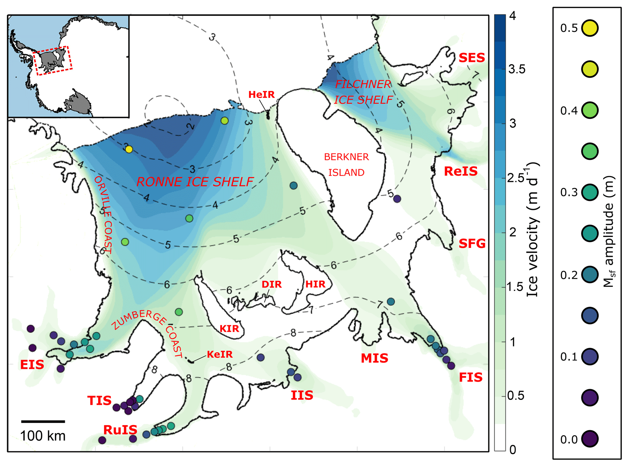
https://www.the-cryosphere.net/14/17/2020/tc-14-17-2020-f01

Figure 1Map showing the Filchner–Ronne Ice Shelf and adjoining ice streams. Circular markers show locations of GPS sites and are coloured according to M_sf amplitude. The background colour map shows ice speed, grounding lines are indicated by solid black lines and dashed contour lines show tidal range (in metres). Acronyms for glaciological features marked on the map are as follows: Evans Ice Stream (EIS), Talutis Ice Stream (TIS), Rutford Ice Stream (RuIS), Institute Ice Stream (IIS), Moller Ice Stream (MIS), Foundation Ice Stream (FIS), Support Force Glacier (SFG), Recovery Ice Stream (ReIS), Slessor Ice Stream (SES), Hemmen Ice Rise (HeIR), Korff Ice Rise (KIR), Kershaw Ice Rumples (KeIR), Doake Ice Rumples (DIR) and Henry Ice Rise (HIR).

1.1 Ocean tides beneath the Filchner–Ronne Ice Shelf

Tidal models constrained by GPS observations have led to accurate knowledge of vertical tidal motion beneath the Filchner–Ronne Ice Shelf (Padman et al., 2002). Vertical tides at the grounding lines of ice streams feeding into the Ronne Ice Shelf are the largest in Antarctica, with a tidal range of up to 8 m (Fig. 1, dashed contours), making this an ideal location to investigate tidal effects on ice shelf flow.

Vertical tidal motion can be split into many tidal constituents, each with a unique period. Of these constituents, the semidiurnal M₂ (principal lunar) and S₂ (principal solar) constituents have the largest amplitudes in this region. They are characterised by an amphidromic point, where their amplitude is zero and around which they rotate, located near the centre of the Ronne Ice Shelf front. These two constituents have periods of approximately 12.42 and 12 h, respectively, and their combined wave envelope gives rise to the spring–neap tidal cycle. This wave envelope should not be confused with the M_sf frequency, despite having the same apparent “period” of 14.76 d. The M_sf frequency is found in spectral analysis of horizontal ice shelf and ice stream displacements but not in the vertical tidal motion, since the semidiurnal wave envelope contains no energy at a fortnightly period. In addition to the important semidiurnal constituents, two diurnal constituents (O₁ and K₁) also have relatively large amplitudes, increasing near the grounding lines. Unlike the semidiurnal constituents, these do not rotate around an amphidromic point, and instead their phase increases approximately linearly through the region, from east to west.

1.2 Observations of tidally modulated horizontal ice shelf displacement

The first GPS observations to find tidal modulation of horizontal ice shelf flow were made in the Ekström Ice Shelf grounding zone (Riedel et al., 1999). In the years since, similar observations have been made on the Brunt (Doake et al., 2002; Gudmundsson et al., 2017 a), Ross (Brunt et al., 2010), Larsen C (King et al., 2011), and Filchner–Ronne ice shelves (Makinson et al., 2012; Rosier et al., 2017 a) and the Mertz and Langhovde glacier tongues (Legresy et al., 2004; Minowa et al., 2019). In terms of ice shelf velocities, different tidal constituents dominate depending on the local tidal regime. For example, in the Ross sea, the diurnal constituents (O₁ and K₁) dominate the vertical ocean tidal signal and the (horizontal) ice shelf flow response. Conversely, in the Weddell Sea, the semidiurnal constituents are strongest in both the vertical (Sect. 1.1) and horizontal motion (Makinson et al., 2012).

In this study, we focus our modelling efforts on the Filchner–Ronne Ice Shelf, where we have a relatively large number of observations and the largest (vertical) ocean tidal amplitudes in the whole of Antarctica. A network of nine GPS stations made measurements spanning over a year in locations both near the Ronne ice front and further into the shelf (Makinson et al., 2012). These GPS measurements reveal strong horizontal tidal modulation at diurnal and semidiurnal frequencies. During the spring tide, at sites near the ice front, horizontal velocity and strain varied by ±300 % of the mean values over a tidal cycle, periodically causing direction of flow to be reversed (Makinson et al., 2012). Further upstream from the calving front, horizontal diurnal and semidiurnal signals were found to decay to almost zero.

A more recent study, which included several additional GPS sites deployed for up to a year near the outlet of major ice streams feeding the Ronne Ice Shelf, found that the response over semidiurnal and diurnal periods increased again towards the grounding lines (Rosier et al., 2017 a). Further analysis of all available GPS data also revealed a strong M_sf component in horizontal ice shelf displacements across the entire floating ice shelf (Rosier et al., 2017 a). This signal had previously been found on grounded ice streams (Gudmundsson, 2006; Minchew et al., 2016) and at a few locations on the Larsen C and Brunt Ice Shelves (King et al., 2011; Gudmundsson et al., 2017 a) but has now been found to occur over a vast area and with an amplitude typically greater than had been found on ice streams (Rosier et al., 2017 a).

1.3 Proposed mechanisms for tidal modulation of ice shelf flow

With the realisation that tides can strongly modulate ice flow, many different mechanisms have been put forward to explain these observations. Initially, Doake et al. (2002) suggested that currents beneath the Brunt Ice Shelf could be responsible for the tidal signals found there, and this idea was explored further by Legresy et al. (2004) and Brunt and MacAyeal (2014). More recently, the discovery of an M_sf signal far upstream of the RuIS (Rutford Ice Stream) grounding line (Gudmundsson, 2006) has led to a focus on replicating these observations (Gudmundsson, 2007, 2011; Rosier et al., 2014, 2015; Minchew et al., 2016) and much less has been done to understand the origin of horizontal tidal signals on ice shelves.

The large horizontal semidiurnal modulation of the Filchner–Ronne Ice Shelf flow was discovered by Makinson et al. (2012), who suggested that it could be explained by an elastic response to tilting of the ice shelf as tides rotate around the amphidromic point. On the Ross Ice Shelf, Brunt and MacAyeal (2014) used a purely viscous model to explore the effects of both tilt and currents but found that they could not replicate GPS observations. Neither of these studies investigated longer period modulation of ice shelf flow.

Efforts to understand the cause of the long period M_sf signal, now known to occur across many of the Antarctic ice shelves for which we have GPS data, require a non-linear mechanism (Gudmundsson, 2007). The paucity of observations of this type on ice shelves led for some time to an implicit assumption that any M_sf signal observed on ice shelves was transmitted directly from grounded ice rather than generated in floating regions. The increasing number of observations of the M_sf signal, revealing that in at least some cases the phase leads and amplitude are greatest downstream of grounding lines, have made it clear that additional mechanisms must be at play (Minchew et al., 2016; Rosier et al., 2017 a).

One possible non-linear mechanism is that vertical tidal motion causes the grounding line to migrate back and forth sufficiently far as to have an effect on ice flow. Evidence of tidal migration of grounding lines remains relatively sparse, but measurements of this process have been inferred via remote sensing (Schmeltz et al., 2001; Brunt et al., 2011; Milillo et al., 2017) and cryoseismicity (Pirli et al., 2018). This could give rise to several non-linearities: firstly, this can result in the width of the ice shelf changing as the portion of floating ice changes over one tidal cycle (Minchew et al., 2016). In addition, the grounding line migration may be asymmetric (Tsai and Gudmundsson, 2015), resulting in a greater migration upstream during high tide than downstream during low tide (Rosier et al., 2014). Another consequence of tidally induced grounding line migration was explored by Robel et al. (2017), who suggested that changes in buttressing arising from grounding line migration could explain observations on RuIS.

An alternative mechanism, termed “flexural ice softening”, that results directly from the non-linear rheology of ice itself, was put forward by Rosier and Gudmundsson (2018). The authors showed that tidal bending stresses in the grounding zone, which will vary in magnitude over a tidal cycle, could lead to a sufficiently large change in the effective viscosity of ice in this region such that ice flow would be enhanced at high and low tide and lead to modulation of ice shelf flow at the M_sf frequency. Each of these non-linear mechanisms could be playing a role in generating the observed M_sf signal.

Our main objective in this paper is to narrow down the possible causes of observed tidal motion of the Filchner–Ronne Ice Shelf by quantifying the contributions of several different processes using a 3-D viscoelastic model and comparing these results with observations. In particular, we will focus on modelling the two strongest responses observed in horizontal ice shelf flow: at the M₂ and M_sf frequencies.

2 Methods

In this section, we present a description of the 3-D full Stokes viscoelastic model used to investigate tidal modulation of ice shelf flow. What is described below is what we call the “default setup”. Several model experiments necessitated modifications or additional features of this setup, and these differences are stated explicitly below. The various model versions that arise due to these differences are listed in Table 1 and each is explained in more detail in the relevant appendix.

Table 1Overview of the various model versions, including a brief description of how each one differs from the default setup and the relevant appendix in which more details can be found.

Download Print Version | Download XLSX

2.1 Field equations

We use a 3-D full Stokes viscoelastic model in a Lagrangian frame of reference to solve for conservation of mass, linear momentum and angular momentum (respectively):

\begin{array}{l} (1) & \frac{D ρ}{D t} + ρ v_{i, i} = 0, \\ (2) & σ_{i j, j} + f_{i} = 0, \\ (3) & σ_{i j} - σ_{j i} = 0, \end{array}

using the commercial finite-element analysis software MSC.Marc (MSC, 2017). In the equations listed above, D∕Dt is the material time derivative, v_i is the components of velocity, σ_ij is the components of the stress tensor, ρ is the ice density and f_i is the components of the gravity force. We use commas to denote partial derivatives with respect to the spatial coordinates and the summation convention for indices.

Ice rheology is represented by an upper-convected Maxwell model (e.g. Gudmundsson, 2011) that relates deviatoric stresses τ_ij and deviatoric strains e_ij with

\begin{matrix} (4) & {\dot{e}}_{i j} = \frac{1}{2 G} {\overset{▿}{τ}}_{i j} + A τ_{E}^{n - 1} τ_{i j}, \end{matrix}

where A is the rate factor, $τ_{E} = \sqrt{τ_{i j} τ_{j i} / 2}$ is the effective stress, n is the constant in the Glen–Steinemann flow law (Steinemann, 1954; Glen, 1955), G is the shear modulus

\begin{matrix} (5) & G = \frac{E}{2 (1 + ν)}, \end{matrix}

ν is the Poisson's ratio and E is the Young's modulus (Shames and Cozzarelli, 1997). The superscript ▿ denotes the upper-convected time derivative, i.e.

\begin{matrix} (6) & \overset{▿}{τ} = \partial_{t} τ + v \cdot ▿ τ - (▿ v)^{T} \cdot τ - τ \cdot ▿ v, \end{matrix}

and deviatoric stresses and strains are defined by

\begin{matrix} (7) & τ_{i j} = σ_{i j} - \frac{1}{3} δ_{i j} σ_{k k}, \end{matrix}

and

\begin{matrix} (8) & e_{i j} = ϵ_{i j} - \frac{1}{3} δ_{i j} ϵ_{k k}, \end{matrix}

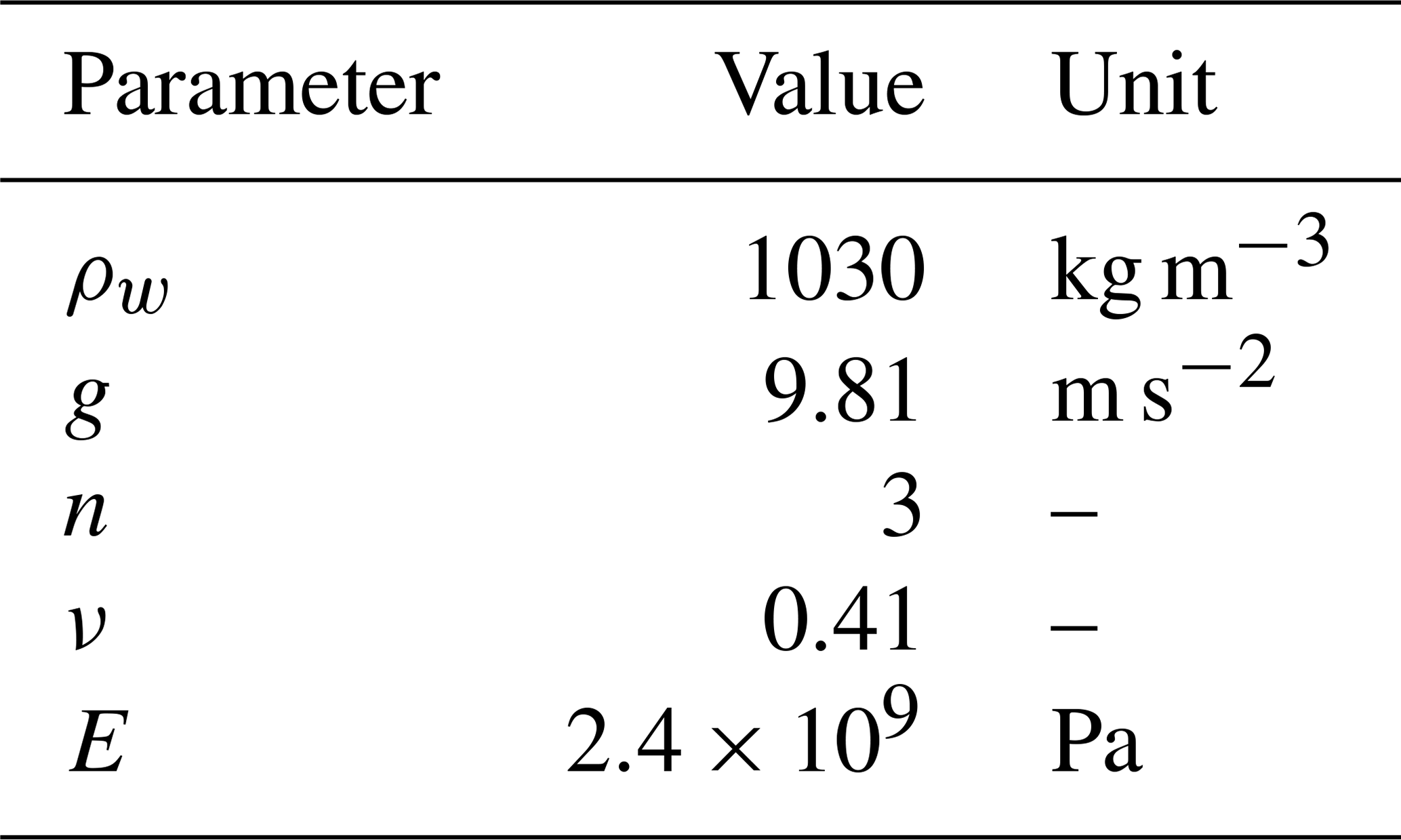
respectively, where ϵ_ij are the components of the strain tensor and δ is the Kronecker delta function. In all simulations we use a value for the Poisson's ratio of 0.41, in line with previous studies (Gudmundsson, 2011; Rosier et al., 2014, 2017 a), and this choice has no effect on our results. The rate factor is inverted for via the adjoint method implemented in the Úa ice flow model (Gudmundsson et al., 2012) to match observed surface ice velocities (Rignot et al., 2017, 2011 a; Mouginot et al., 2012), as outlined in Appendix A, and the resulting velocity field is shown in Fig. 2c. The model parameter choices for the default setup are shown in Table 2. The rheological equations are solved implicitly with a time step that changes adaptively based on a target number of iterations to reach the convergence criteria. The rheology outlined above is modified in three of the experiments. The RF_Burgers experiment uses a Burgers rheology (Appendix D), the RF_temperature experiment makes A a function of temperature (Appendix G) and the RF_damage experiment adds a damage term in the elastic component of the Maxwell rheology (Appendix C).

2.2 Boundary conditions

At the base of the ice shelf and along the ice front, a pressure is applied normal to the element faces given by

\begin{matrix} (9) & p = \{\begin{cases} ρ_{w} g (S (x, y, t) - z (t)) & if z (t) < 0 \\ 0 & otherwise, \end{cases} \end{matrix}

where ρ_w is the sea water density, $S (x, y, t)$ is the time-varying local sea level (Sect. 2.3) and z is the height above sea level. At the ice surface, a stress-free boundary condition is imposed such that

\begin{matrix} (10) & σ \cdot n = 0, \end{matrix}

where n is the unit vector normal to the boundary. The only other boundary condition (BC) necessary in this default setup is along the grounded sidewalls of the ice shelf domain. A Dirichlet BC is imposed on nodes along the grounded edge of the model, such that

\begin{matrix} (11) & u = u_{obs}, v = v_{obs}, w = 0, \end{matrix}

where w is the vertical ice velocity and u_obs and v_obs are observed horizontal ice velocities (Rignot et al., 2017, 2011 a; Mouginot et al., 2012) and constant in time. This BC allows for inflow from fast-moving ice streams but clamps nodes vertically at the grounding line such that ice in the grounding zone must bend to accommodate vertical tidal motion of the ice shelf. Another result of using this Dirichlet BC is that the grounding line (GL) cannot migrate in these simulations; however, later we will introduce a different model setup in which this constraint is loosened. We use Bedmap2 (Fretwell et al., 2013) to define the model geometry; including ice thickness, ice surface elevation and grounding line position.

Table 2List of model parameter choices for the default model setup.

Download Print Version | Download XLSX

2.3 Tidal forcing

We use the circum-Antarctic inverse model (referred to hereafter as CATS2008a, which is an updated version of the inverse tidal model described by Padman et al., 2002) to force our viscoelastic model at the ocean boundary with vertical tidal motion. By most measures, CATS2008a remains the best-performing tidal model in this region (King et al., 2011). The CATS2008a model includes 10 tidal constituents and we opt to force our model with the four largest constituents in the region by amplitude (M₂, S₂, O₁ and K₁), representing the principal semidiurnal and diurnal constituents. With these four constituents the most important tidal features are captured, such as the spring–neap cycle and the rotation of tides around the Weddell Sea amphidromic point. The fortnightly M_sf signal is produced through interaction between the M₂ and S₂ constituents and we include the diurnal constituents to ensure that the total tidal range is close to what is observed. The advantage of forcing the model with only these four constituents is to ensure that any other tidal frequencies that arise in the model must be generated through internal processes rather than directly from the forcing. The tidal model domain uses a slightly different grounding line to that used in the model presented herein, particularly at the outlet to Evans Ice Stream, so interpolation is done to fill in areas with no amplitude or phase information in CATS2008a.

2.4 Element discretisation

The finite-element mesh uses 3-D, 15-node, isoparametric pentahedrons, arranged such that the triangular faces are orientated in the horizontal plane (Fig. 2b). The pentahedral shape is well suited to modelling an ice shelf in three dimensions, since the triangular faces enable the element to conform to a complicated coastline geometry without an excessive number of elements and the relatively flat surfaces of the ice shelf are captured well with the quadrilateral faces. The stiffness of the element is formed using 21-point Gaussian integration, and triquadratic interpolation shape functions are used for displacements, resulting in a linear variation in stress through the element. The model mesh, generated using mesh2d (Engwirda, 2014), is unstructured and refined around grounding lines and in regions of high lateral shear strain (Fig. 2a). Certain model versions necessitate a different mesh, but the total number of elements remains approximately the same and results in between 5×10⁵ and 1×10⁶ degrees of freedom.

To test the effects of mesh resolution on our model results we ran simulations in which horizontal and vertical mesh resolution were doubled. The main differences in modelled M_sf amplitude are confined to the grounding zone, with a maximum change in amplitude across all nodes of 1 cm. Over the bulk of the shelf, the difference in M_sf amplitude between the simulations was typically of order 1 mm or less. Similarly, differences in the horizontal M₂ signal were limited to the grounding zone, with higher resolution resulting in similar amplitudes but a more confined band of tidal motion at this frequency.

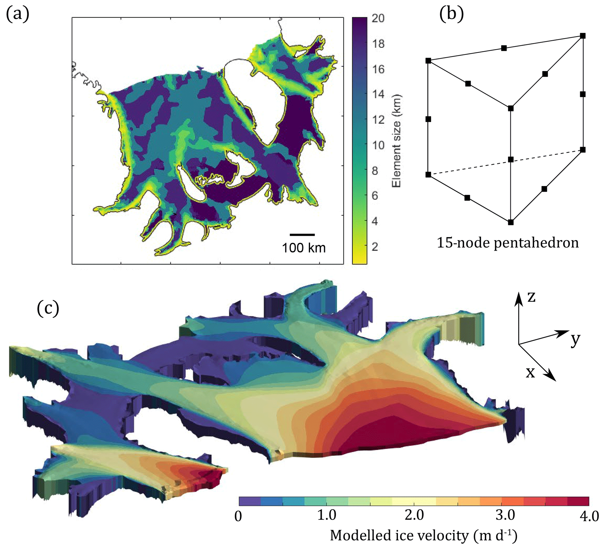
https://www.the-cryosphere.net/14/17/2020/tc-14-17-2020-f02

Figure 2Overview of the finite-element model, showing model resolution (a), the quadratic pentahedral elements used (b) and a vertically exaggerated oblique view of the model showing modelled mean ice velocity for the default setup experiment (c).

3 Results

A number of different model setups were used in the course of this study. Our strategy, whose motivation will become clear later, was to begin by attempting to reproduce GPS observations of horizontal tidal displacements at the principal semidiurnal (M₂) frequency. Once the model was able to reproduce these observations we subsequently searched for the source of the fortnightly (M_sf) frequency by testing a number of mechanisms and parameter combinations. Our results are, therefore, structured in that order and we begin by presenting model results at the M₂ frequency. In all cases, the two horizontal components of modelled surface nodal displacements were processed using the UTide MATLAB package (Codiga, 2011). This state-of-the-art tidal analysis software calculates amplitudes of tidal constituents using an iteratively reweighted least-squares method and our model results are largely presented in terms of the semi-major axis amplitude of each constituent.

3.1 Semidiurnal (M₂) results

Modelled horizontal ice shelf displacements at the M₂ frequency only differed slightly between all the model experiments set out in Table 1 and thus we only present the M₂ results from the default setup. A large amplitude M₂ component in modelled ice shelf flow is found around most grounding lines and towards the ice shelf front (modelled M₂ amplitude is shown by the main colour map in Fig. 3). The maximum in the modelled M₂ signal is focused around the M₂ amphidromic point, near the centre of the ice shelf front, where the amplitude approaches 0.5 m.

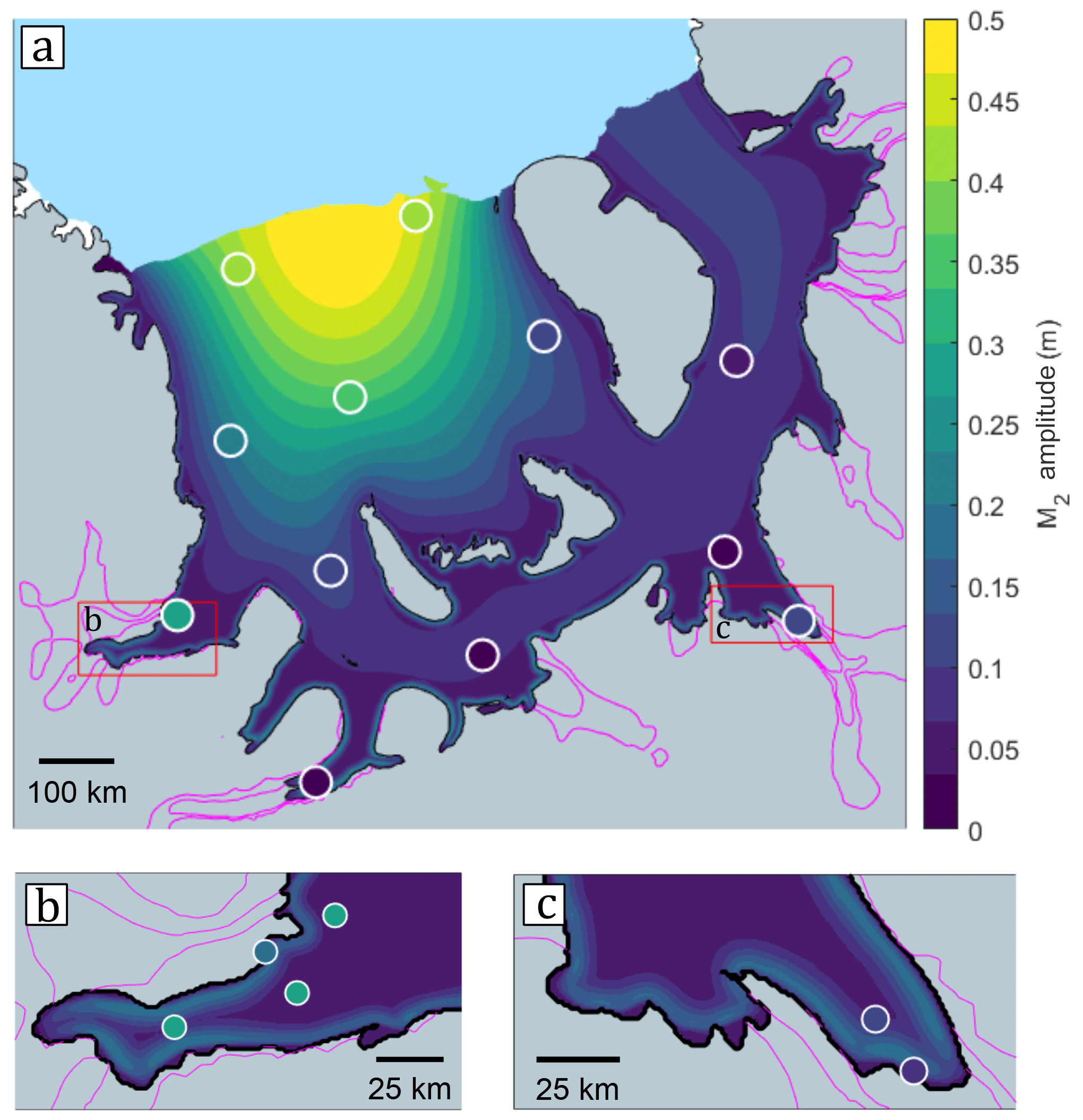
https://www.the-cryosphere.net/14/17/2020/tc-14-17-2020-f03

Figure 3Amplitude of modelled horizontal ice shelf displacements at the M₂ frequency (background colour map) compared with GPS observations (circles). Magenta lines are 0.5 m d⁻¹ ice velocity contours, to help identify regions of fast flowing grounded ice. Grounded ice and open ocean are coloured grey and blue, respectively, and ice shelves not included in the model domain are white. Panels (b) and (c) show magnified maps of EIS and FIS, respectively. Additional GPS sites are shown in these sub-panels that are not shown in panel (a) for the sake of clarity.

The difference between the modelled and observed response at the M₂ frequency is small over the majority of the ice shelf (GPS observations of M₂ amplitude are indicated by coloured circles in Fig. 3, using the same colour scale as the background colour map). In particular, the bulk signal revealed by GPS observations of increasing amplitude towards the ice front is reproduced by the model. The only discrepancy occurs at GPS locations located near grounding lines but outside of the immediate grounding zone. GPS observations at these locations reveal a stronger amplitude M₂ signal than that generated in the model, where it largely remains confined to the narrow grounding zone (Fig. 3). This mismatch is largest around the outlet of EIS, where modelled M₂ amplitude is ∼ 30 % of the value measured by GPS (Fig. 3b). Any horizontal tidal motion must decay to zero at the grounding line as a result of our model BCs and so this mismatch is alleviated somewhat in experiments where this constraint is removed (described later).

A number of model experiments were conducted specifically to better understand the model response at the M₂ frequency. Firstly, the Young's modulus was both increased and decreased (between 1 and 9 GPa) to investigate how this affects the M₂ signal. This was found to only alter the amplitude of the M₂ effect and not its spatial variability; an increase in E reduced the amplitude and vice versa for a decrease in E. Since the modelled M₂ amplitude is only sensitive to E, we treat it as a tuneable parameter and found that a value of E=2.4 GPa produced a very good fit to observations.

Two further model experiments were carried out to confirm the mechanisms responsible for generating this M₂ signal in the model. Neither of these experiments are realistic, in the sense that the model boundary conditions are not consistent with observations, and they only serve to better understand the model behaviour. In the first, the vertical Dirichlet boundary condition imposed along the sides of the ice shelf was removed. In this experiment, the bulk M₂ signal across the majority of the shelf was identical but no M₂ signal was generated in the grounding zone since bending effects were removed. The second experiment set the amplitude and phase of all tidal constituents to be the same in the whole domain (equal to the mean amplitude in this region). This stops the ice shelf from tilting due to spatial variation in either tidal amplitude or phase. With this setup the model only generates an M₂ signal in the grounding zone and there is no horizontal displacement at the M₂ frequency across the main bulk of the ice shelf. These two additional experiments hence confirm that the M₂ signal is primarily generated through ice shelf tilting with a small localised component generated near grounding lines due to tidal flexure.

3.2 Lunar synodic fortnightly (M_sf) results

Having identified the mechanism responsible for generating the M₂ signal and having selected an appropriate value for E, we now turn our attention to the M_sf signal. A number of model experiments were conducted, including various different processes (as outlined in Table 1) in an effort to determine possible sources of the observed fortnightly (M_sf) modulation in flow of the Filchner–Ronne Ice Shelf. These runs can broadly be split into two categories; those in which the flexural softening mechanism is primarily responsible for generating an M_sf signal and those that allow the GL to move and in which tidally induced GL migration is the primary mechanism at play.

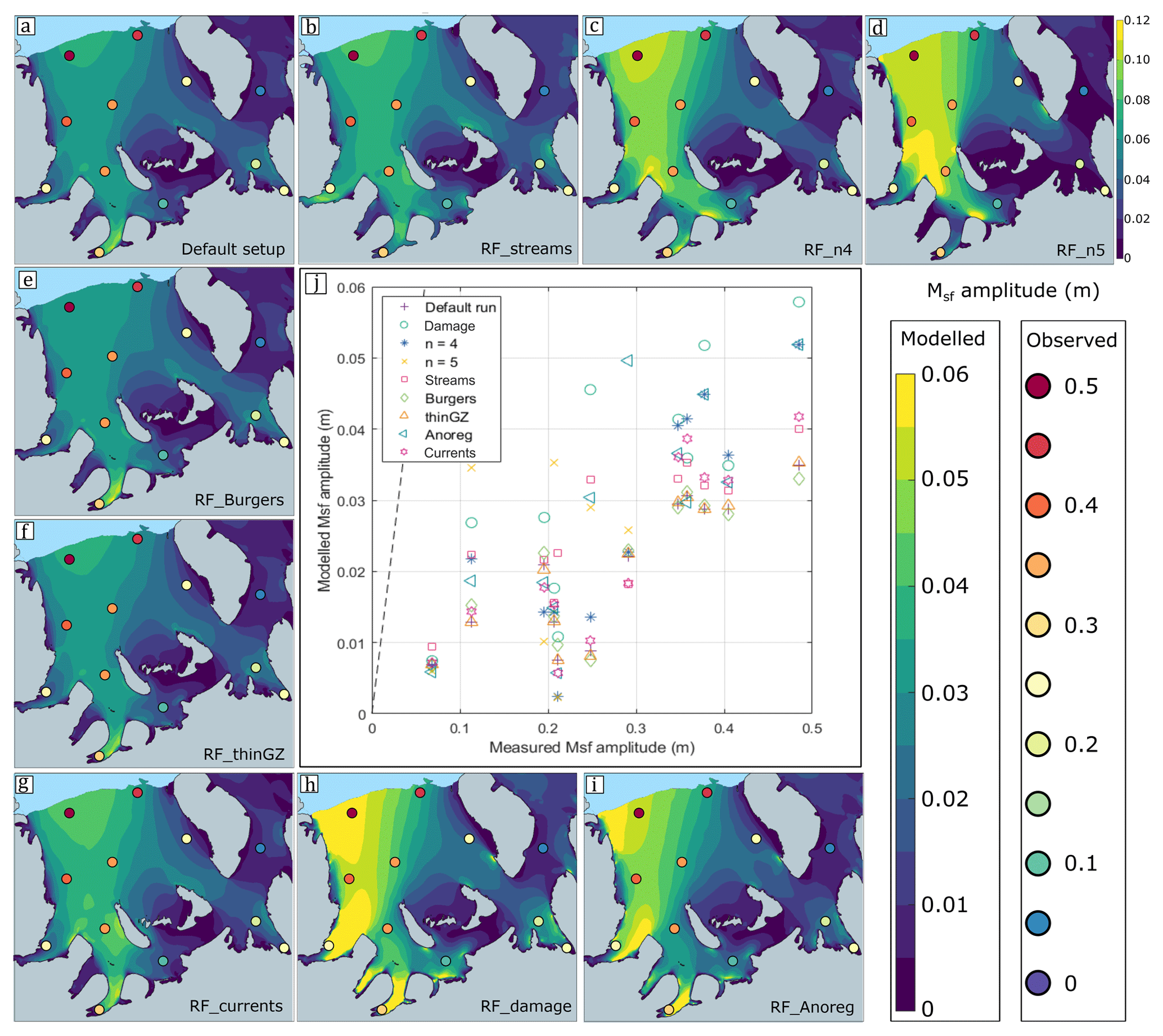
https://www.the-cryosphere.net/14/17/2020/tc-14-17-2020-f04

Figure 4M_sf amplitude on the Ronne Ice Shelf for nine of the model experiments (a–i) outlined in Table 1. Note the different colour scale used for experiment “RF_n5” in panel (d). Observed M_sf amplitudes from GPS observations are indicated in panel (a) by coloured circles. Panel (j) compares measured and modelled M_sf amplitude at each of the marked locations for the same set of experiments. Note that in producing this figure we use an evenly distributed subset of measurements to avoid bias in areas with more measurements and thus make interpretation of the overall misfit across the entire ice shelf easier.

3.2.1 Flexural softening experiments

The strength of the M_sf signal generated through the flexural softening mechanism, as proposed by Rosier and Gudmundsson (2018), is sensitive to a number of different modelling choices. We explore whether any of these could yield an M_sf signal similar to observations and the results of these model simulations are shown in Fig. 4. Firstly, the “default_setup” experiment produces an M_sf response whose spatial distribution appears to agree reasonably well with GPS measurements, but the amplitude is much smaller than observed (Fig. 4a). For example, towards the ice shelf front, where the M_sf signal has a measured amplitude of ∼ 0.5 m, the modelled M_sf amplitudes are about an order of magnitude smaller. Similarly poor numerical fit to observations is found around the grounding zones, where a large number of GPS observations exist. We thus conclude that although the default setup produces a realistic looking spatial variation in M_sf amplitudes, either the parameter values used are incorrect, or some essential physics are missing. To identify the cause of the misfit, we start by investigating the sensitivity of the modelled response to various parameter values.

Since it is the non-linear aspect of ice rheology that drives the flexural softening mechanism and gives rise to the non-linear M_sf response, we start by changing the value of the ice flow stress exponent. Increasing the exponent in the Glen–Steinemann flow law from n=3 to n=4 (Fig. 4c) or n=5 (Fig. 4d; note the different colour scale used for this panel) increases the M_sf amplitude substantially; however, it is not in a manner sufficient to match observations. We tested the use of the more complex Burgers rheology, which includes the delayed elastic response (Appendix D), but this only led to a 5 %–10 % change in the M_sf amplitude compared to that of the default_setup (Fig. 4e). We then tried several different spatial distributions of the rate factor A. For example, in the “RF_Anoreg” experiment, we used a different rate factor field to in the default setup, which was obtained through inversion of surface velocities using the ice flow model Úa, but this time without any regularisation (Appendix A). The resulting M_sf amplitude is generally larger than the default_setup, particularly along the western margins in the domain with a high spatial heterogeneity in the rate factor field where modelled M_sf amplitudes are increased by ∼ 50 % but are still much smaller than observations (Fig. 4i). Thus, despite changing the value of the ice flow stress exponent n, changing the distribution of the rate factor A and using an alternative rheological model, we were not able to match the observed M_sf amplitudes.

The geometry used in the default_setup model assumes hydrostatic equilibrium to calculate ice shelf thickness from known surface elevation, but this assumption breaks down near grounding lines where bridging stresses become important. Since the bending stresses that generate an M_sf signal in the default_setup are sensitive to ice thickness in the grounding zone, we conduct the “RF_thinGZ” experiment in which ice thickness is reduced in this region, as outlined in Appendix H. This change in geometry only has a small impact on the overall M_sf amplitude (Fig. 4f). Crevassing in the grounding zone could also reduce the effective stiffness of ice and thereby alter the magnitude of tidal bending stresses. In the “RF_damage” model experiment, we adopt a continuum damage mechanics approach to simulate this effect (Appendix C). This experiment has a more profound effect on effective ice stiffness and thus leads to larger changes in the M_sf amplitude (Fig. 4h), but once again these are too small to match observations.

Various authors have suggested that sub-ice-shelf tidal currents could play a role in modulating horizontal ice velocities at tidal frequencies (Doake et al., 2002; Legresy et al., 2004). We use tidal currents from the CATS2008 tidal model (Padman et al., 2002) and apply the resultant time-varying drag to the base of the ice shelf in the “RF_currents” experiment, as described in Appendix F. We ran the model with two different drag coefficients, a “canonical” value of $3 \times 10^{- 3}$ and an “extreme” value of $3 \times 10^{- 2}$ . Modelled M_sf amplitude when using the higher drag coefficient is shown in Fig. 4h. These results reveal that strong tidal currents in combination with high drag coefficients could be locally important, increasing M_sf amplitudes in some areas by over 10 % compared to the default_setup. Overall, however, the effect of adding this mechanism is far too small to explain observations, even when using an extreme upper-range value for the drag coefficient.

All of the experiments described above use a constant velocity boundary condition along grounding lines. As a consequence, amplitudes of any temporal variations in ice flow go to zero towards the edges of the computational domain. In order to verify that this choice of boundary condition does not significantly affect the tidal response of our model over the main bulk of the ice shelf, we conducted further modelling experiments where the boundaries of the computational domain were placed further upstream within all the main ice streams flowing into the Filchner–Ronne Ice Shelf. This setup is referred to as the “RF_streams” setup and is described further in Appendix B. In the RF_streams setup, the lateral extent of these additional grounded regions is chosen so that ice velocity along their boundary is approximately zero, while their upstream extent is chosen to be further than any observed tidal effects in the region (i.e. > 100 km). We find that around the grounding lines of major ice streams this leads to an increase in the M_sf amplitude. However, over the majority of the shelf the differences between the two simulations are generally less than 10 % (Fig. 4c). Since including the grounded ice streams greatly increases the computational cost of running the model and we are focusing on replicating GPS observations across the main shelf, we use this result to justify omission of grounded ice in our domain in all other numerical experiments.

3.2.2 Grounding line migration experiments

None of the numerical experiments described above were able to reproduce the observed M_sf amplitudes and despite all our efforts modelled M_sf amplitudes are only about 10 % of observed values. This suggests that hitherto we may have not included the physical mechanism responsible for generating the observed M_sf signal in our model. We stress that we have, however, been able to reproduce the spatial pattern and the amplitudes of the short-period (horizontal) tidal modulation in flow, as well as the spatial pattern in the long-period tidal modulation.

We now include a physical mechanism that has, until now, been missing from our modelling efforts. This mechanism involves grounding line migration in response to tides. We use the “RF_GLmigration” model version to run several experiments that explore the role of this mechanism in generating the pervasive M_sf signal observed on the Filchner–Ronne Ice Shelf. Since the amount by which the grounding line will migrate is highly dependent on local bed slopes, of which we have very poor knowledge, we implement this mechanism using the simple analytical approach derived by Tsai and Gudmundsson (2015). In essence, upstream and downstream migration distances are generally expected to be different and can be written as $Δ L^{+} = Δ S^{+} / γ^{+}$ and $Δ L^{-} = Δ S^{-} / γ^{-}$ , where L is migration distance and the positive or negative indices indicate positive or negative vertical tidal motion. Two parameters control the distance that the GL migrates up or downstream, γ⁺ and γ⁻, which determine the upstream and downstream migration distance, respectively, as a function of local tidal height (ΔS). A more detailed description of our implementation of this mechanism can be found in Appendix E. With GL migration modelled in this way, the experiments that follow include several effects that could generate an M_sf signal: asymmetric grounding line migration, temporal variations in buttressing, and periodic narrowing and widening of the ice shelf.

A simulation using $γ^{+} = 6 \times 10^{- 4}$ and $γ^{-} = γ^{+} / 7.2$ yields a strong M_sf signal with an amplitude of ∼0.5 m near the ice front, matching reasonably well with observations (Fig. 5a). To help put this in context, this choice of parameters is equivalent to a maximum upstream migration of 5 km (or ∼ 700 m downstream) for a positive (or negative) vertical tidal motion of 3 m (but note that since GL migration is a function of local tidal amplitude, the actual migration distance varies spatially). The migration is asymmetric (since $γ^{+} > γ^{-}$ ), and this degree of asymmetry is within the range that might be expected based on geometric arguments (Tsai and Gudmundsson, 2015). We thus find that this mechanism is capable of producing M_sf amplitudes matching observations.

We can explore what happens to the M_sf amplitude if just the asymmetric component of the grounding line migration non-linearity is removed (i.e. $γ^{+} = γ^{-} = 1.05 \times 10^{- 3}$ ). The resulting M_sf amplitude with a symmetric grounding line migration, but the same total migration distance over one tidal cycle is shown in Fig. 5c. The M_sf amplitude is generally ∼ 50 % smaller than in the asymmetric case, although it is still larger than experiments with no GL migration (Fig. 5d), and certain areas such as the Kershaw Ice Rumples (KeIR) generate a strong M_sf signal.

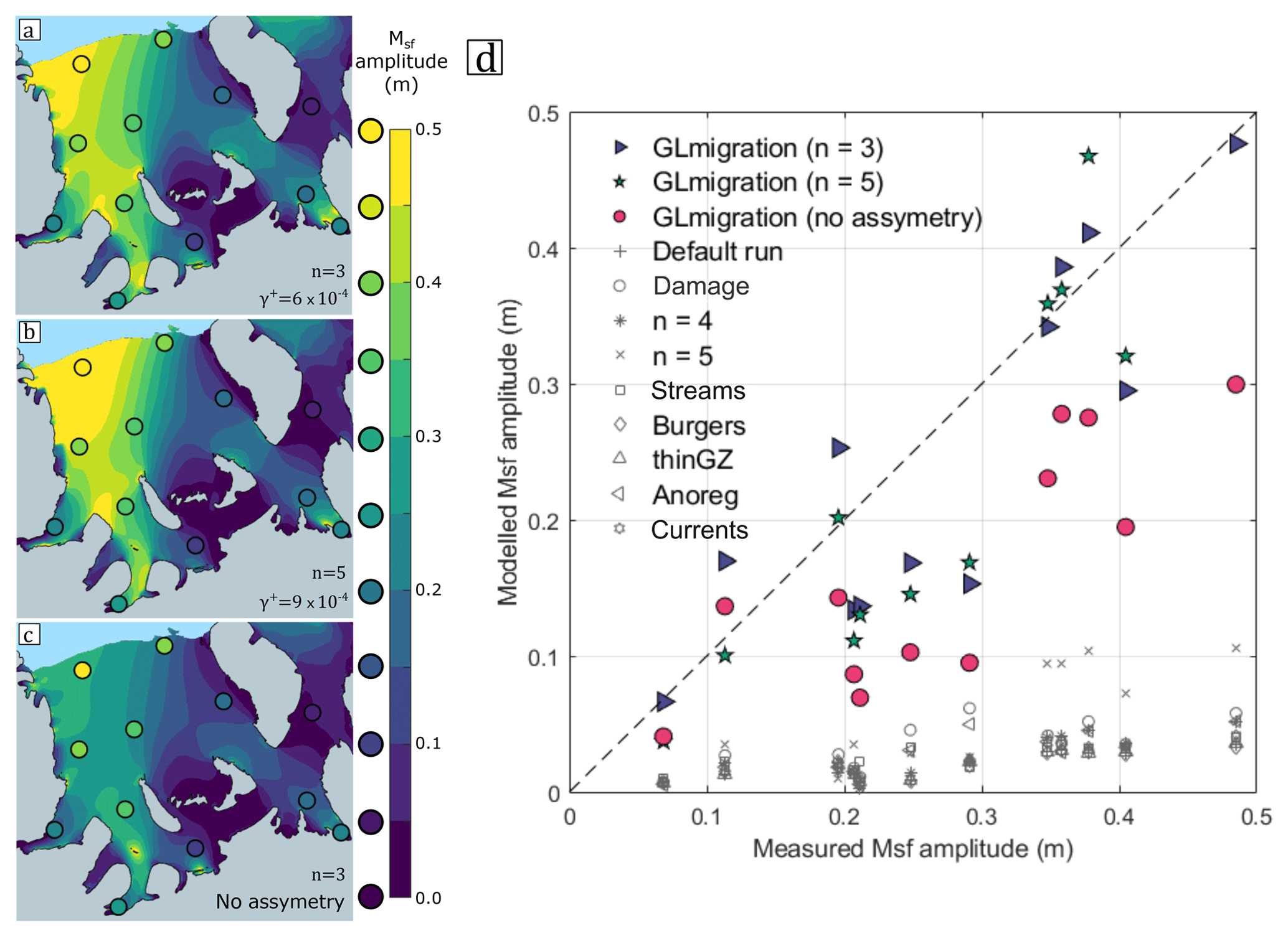
https://www.the-cryosphere.net/14/17/2020/tc-14-17-2020-f05

Figure 5Modelled M_sf amplitude on the Ronne Ice Shelf for three variants of the RF_GLmigration model experiment. Panel (a) uses n=3, $γ^{+} = 6 \times 10^{- 4}$ and $γ^{-} = γ^{+} / 7.2$ , panel (b) uses n=5, $γ^{+} = 9 \times 10^{- 4}$ and $γ^{-} = γ^{+} / 7.2$ , and, finally, panel (c) uses n=3 and $γ^{-} = γ^{+} = 1.05 \times 10^{- 3}$ (i.e. no asymmetric grounding line migration). Observed M_sf amplitude is indicated by the filled circles using the same colour scale. Panel (d) compares measured and modelled M_sf amplitude at each of the marked locations for runs that include the GL migration mechanism (coloured symbols) and those previously presented that do not (grey symbols).

We conduct a final experiment in which we combine the GL migration mechanism with an ice rheology in which n=5 in the Glen–Steinemann law. We explore this particular combination because the choice of n was found to have the next largest effect on M_sf amplitude (Fig. 4d), and this parameter remains poorly constrained (e.g. Cuffey and Paterson, 2010), yet is of great importance to transient ice sheet behaviour. Increasing the exponent in the flow law leads to a larger M_sf signal across the shelf and thus we can obtain an equally good match to the observed M_sf amplitude with a lower γ⁺ of $9 \times 10^{- 4}$ (Fig. 5b). In this case, upstream and downstream migration distances needed to fit observations are 33 % smaller than with a choice of n=3, but qualitatively the spatial pattern of the long-period response is largely unchanged.

4 Discussion

We find that strong modulation of ice shelf flow at the short-period M₂ frequency is generated by tilting of the ice shelf, supporting the hypothesis of Makinson et al. (2012). This tilt occurs through a combination of phase differences in high-tide times around the domain and the lower amplitude vertical tides at the ice shelf front, leading to a rotating tilt vector centred around the M₂ amphidromic point in the Weddell Sea. The modelled amplitude of horizontal ice shelf displacement at M₂ frequency is very similar between all model experiments that used the same elastic rheological parameters and almost completely insensitive to changes in either the viscous ice rheology or the inclusion of other mechanisms such as tidal currents and GL migration. These results demonstrate that the short frequency modulation of ice shelf flow arises from simple linear elastic processes. Tidal current drag has previously been posited as a possible explanation for the modulation of horizontal ice shelf flow (Doake et al., 2002; Legresy et al., 2004; Brunt and MacAyeal, 2014), a mechanism which we can now discount for any reasonable choice of drag coefficient.

The modelled M₂ amplitude was only sensitive to our choice for the Young's modulus (E) and the best fit to GPS observations was found using E=2.4 GPa. This Young's modulus can be thought of as an “effective” value, relevant for tidal periods, since for a viscoelastic material subjected to a periodic forcing, the Young's modulus is a function of loading frequency (Shames and Cozzarelli, 1997). Linear elastic beam models have often been fitted to measurements of tidal flexure to obtain a wide variety of values for the effective Young's modulus of ice (Lingle et al., 1981; Stephenson, 1984; Kobarg, 1988; Smith, 1991; Vaughan, 1995; Schmeltz et al., 2002; Sykes et al., 2009; Hulbe et al., 2016); however, most of these arguably mistakenly treat the resulting E as a material constant and furthermore they are highly sensitive to local factors such as basal crevassing (Rosier et al., 2017 b). The horizontal M₂ frequency ice shelf displacement in our model is generated by strain in the main body of the shelf as it tilts due to differential tidal amplitudes. Therefore, unlike previous studies that rely on very localised measurements, this model provides an excellent opportunity to estimate the viscoelastic properties of ice shelves.

The amplitude of the modelled M_sf response was also found to be sensitive to the Young's modulus, since this changes the bending stresses in the grounding zone. On the other hand, the strength of the short period M₂ signal was effectively independent of any changes in viscous ice rheological parameters and indeed almost any other change made to the viscous model parameters. This finding justifies our strategy of first tuning the elastic properties of the model to match observed M₂ response before moving on to exploring the processes and parameters that play a role in generating the M_sf signal.

Our study investigates the two mechanisms that have been proposed to explain the generation of the M_sf signal across an entire ice shelf: non-linear flexural ice softening and grounding line migration. We test our model results against a comprehensive GPS dataset collected over more than a decade on the Filchner–Ronne Ice Shelf. While the flexural ice softening mechanism is capable of generating an M_sf response, we have found that no tested combination of parameters or further model modifications involving visco-elastic rheological laws or model geometry can produce a sufficiently large amplitude M_sf signal to match observations through this mechanism alone (Fig. 4). This mechanism must be responsible for some of the observed M_sf signal, since the non-linear rheology of ice is well established, but it cannot explain the pervasive and strong M_sf signal that is observed over the entire Ronne Ice Shelf.

On the other hand, we do find that grounding line migration can produce large-amplitude fortnightly modulation in ice shelf flow. Despite the relatively simple implementation employed here, the addition of this process into the model can easily produce an M_sf signal that matches observed M_sf amplitude and the broadscale spatial distribution (Fig. 5a). It would presumably be possible to obtain an exact fit to observations by allowing the grounding zone geometry to vary spatially; however, finding the optimal geometry is a daunting inverse problem beyond the scope of this paper.

Tidally induced grounding line migration can be subdivided into several non-linear effects, which will all play a potential role in generating an M_sf signal: periodic narrowing and widening of the ice shelf, reduction in basal shear stress, reduced buttressing from ice rises and rumples, and grounding line asymmetry. With our modelling approach we cannot address the reduction in basal shear stress that will occur as the grounding line migrates upstream on major outlet glaciers; however, the other three have been tested using the RF_GLmigration model version (Fig. 5).

Grounding line migration has been suggested as the source of fortnightly modulation in ice shelf flow in two previous studies, through its effects on ice shelf width (Minchew et al., 2016) or buttressing stresses (Robel et al., 2017). These studies both showed how a horizontal M_sf signal could be generated on an ice shelf from a vertical semidiurnal tidal forcing but used a number of simplifying assumptions. Here, we have used a 3-D model of the entire region that includes all the stress terms and thus also flexural stresses that are neglected in the two simpler models. This combination of a more complete model and a realistic geometry, together with the numerous remote sensing and in situ GPS observations, enables us to put tighter constraints on any proposed mechanism. Model parameters that, for example, affect the spatial pattern of secular ice flow (e.g. A and n) also impact the modelled temporal variation in ice flow generated through tidal action. As a consequence, several hitherto potential mechanisms for the generation of long-period tidal modulation in ice flow can now be discounted as viable explanations.

Increasing the exponent n in the ice rheology increases the M_sf amplitude, or conversely reduces the distance that the grounding line needs to migrate to match the observed M_sf signal by 33 %. Without better knowledge of the distance that grounding lines are migrating over the entire ice shelf this result cannot be directly used to estimate viscous ice rheology, but obtaining these data is certainly possible (e.g. Schmeltz et al., 2001; Brunt et al., 2011; Milillo et al., 2017). The migration distances we investigate in this modelling study are within the range obtained by satellite estimates; in this region, Brunt et al. (2011) identified areas in which grounding lines were migrating almost 10 km over one tidal cycle.

Several features of the modelled M_sf response for the RF_GLmigration experiment deserve specific mentions. Unsurprisingly, there is virtually no M_sf signal generated in regions where the ice shelf flows slowly, such as behind Berkner Island and Henry Ice Rise. Somewhat more interesting is the lack of an M_sf signal in our modelled results along the eastern coast of the Ronne Ice Shelf, despite a very large M_sf amplitude on the opposite Orville Coast (Fig. 5). This is because the shear margin is located some distance from the grounding line (Fig. 1), meaning that migration of the grounding line is not felt by the main ice shelf (but where the grounding line and shear margin do coincide, at the southern tip of Berkner Island, an M_sf signal is generated). Upon closer inspection, many of the regions that generate a strong M_sf signal coincide with areas where the shear margin is close to the grounding line.

Our implementation of tidally induced grounding line migration is limited in several ways. Most importantly, without accurate knowledge of bed geometry we have had to resort to assuming equal local bed slopes around all grounding lines. In reality, it is likely that in many areas the grounding line migrates only short distances (although conversely we may be underestimating the migration in certain areas). Furthermore, we do not allow the grounding line to migrate in regions of inflow to the ice shelf since our analytical approach would not yield accurate ice velocities across these grounding lines. However, as we are focused on matching the broadscale features of the M_sf signal, and localised M_sf generation is found to decay over relatively short distances (Fig. 5c), these limitations are not expected to affect our main findings. This second point is further supported by remote sensing observations, which show that the M_sf signal is spatially heterogeneous (Minchew et al., 2016).

Several previous studies have shown that the non-linear response to vertical tidal motion which generates the M_sf signal also leads to a change in the mean ice velocity (Gudmundsson, 2007, 2011; Rosier et al., 2014; Rosier and Gudmundsson, 2018). Our regional model, which can broadly replicate the M_sf signal across the Filchner–Ronne Ice Shelf, now allows us to quantify the magnitude of this effect on an ice shelf for the first time. We ran a repeat of the RF_GLmigration experiment but with no vertical tidal forcing and compared the mean velocity in this simulation with that of our best fit to the observed M_sf signal. We find that, averaged across the entire ice shelf, ice flow is enhanced by ∼ 21 % due to the presence of tides. Much of this tidal flow enhancement is confined to certain portions of the shelf where the local enhancement can be much higher, particularly along the Zumberge and Orville coasts, i.e. ice flowing out from IIS, RuIS and EIS. This suggests that a potentially important feedback exists between tidal amplitude and ice shelf geometry; i.e. if the ice shelf were to thin or retreat it would alter tides sufficiently to further compound changes in ice flow.

5 Conclusions

We are able to obtain a good agreement between our model and observations of short-period tidal modulation in horizontal flow. This study, therefore, allows us to confirm the previously untested theory of Makinson et al. (2012), i.e. that this behaviour arises from the linear elastic response of ice to changes in slope resulting from the relatively high-frequency semidiurnal tides. We are also able to replicate, here for the first time, the size and spatial pattern of the observed long-period (i.e. longer than a day) horizontal motion of the Filchner–Ronne Ice Shelf by including a non-linear mechanism related to grounding line migration over tidal cycles. As with other non-linear mechanisms proposed previously, this involves a non-linear energy transfer from the two main semidiurnal tidal constituents (M₂ and S₂) to the long-period M_sf tidal constituent.

A non-linear response to tidal bending stresses has been previously proposed as a possible mechanism to explain observed long-period horizontal motion (Rosier and Gudmundsson, 2018) and in our model this does produce the same general type of a response. However, our large-scale modelling approach using realistic geometry of the Filchner–Ronne Ice Shelf shows that the generated long-period amplitude is too small and its spatial pattern is inconsistent with observations. We thus arrive at the lateral migration of grounding lines over a tidal cycle as the most promising candidate for explaining the observations of tidal modulation on Filchner–Ronne ice shelf.

In our model, the lateral migration of grounding lines gives rise to several different non-linear mechanisms that all act together. First, the horizontal migration distance is an asymmetrical function of vertical tidal amplitude (this aspect of grounding line migration arises whenever the ice-thickness gradient changes across the grounding line), and this is an example of a geometrical non-linearity. Secondly, ice shelf flow is a non-linear function of width and stress for non-Newtonian fluid such as ice. This suggests that observations of tidal modulation of ice shelf flow can be utilised to extract information about rheology of ice. However, this can only be done if bed geometry and ice thickness across the grounding line are sufficiently well known to calculate the migration distance. Alternatively, if independent observations of lateral migration of grounding lines in response to tides are available, the migration distance can be prescribed directly, in which case the stress exponent (n) can be solved by using a fairly simple modelling approach. Using tidal observations in this manner to extract information about ice rheology is an intriguing possibility that needs to be explored further.

Appendix A: Inversion for ice rate factor

In order to conduct our 3-D tidal model experiments we need to ensure that the model reproduces the observed mean ice flow across the whole computational domain. This we achieve by inverting for the spatial distribution of the rate factor A for any given value of the stress exponent n. Rather than conducting this inversion using our computationally demanding MSC.Marc full Stokes finite-element model, we perform this inversion step using the vertically integrated ice flow model Úa.

The Úa ice flow model uses the finite-element method to solve the shallow shelf (SSA) equations (e.g. Hutter, 1983; MacAyeal, 1989), as described in more detail in Gudmundsson et al. (2012). The inversion procedure that we use in the Úa model seeks to minimise the misfit between observed and modelled surface velocities by minimising log A, using the adjoint method to calculate the gradient of the cost function as first described for ice flow models by MacAyeal (1992, 1993). The cost function being minimised also contains a Tikhonov regularisation term penalising large spatial gradients in log A. For all but one of our simulations we determine the amount of regularisation in our inverted field through an L-curve analysis. We also did experiments without any regularisation (RF_Anoreg experiment).

Using Úa, the inversion procedure was conducted for a much larger domain than that of the full Stokes model, including the entire drainage basin of the Filchner–Ronne Ice Shelf and for flow exponent values of n=3, n=4 and n=5. The inversion algorithm was run for several hundred iterations until the change in cost function in each successive step was below some small tolerance value. The mean absolute difference between observed and modelled surface velocities after the completion of the inversion (for the n=3 inversion with regularisation) was 18.3 m a⁻¹ over the entire domain and 22.5 m a⁻¹ across just the ice shelf. Since the assumptions of the SSA, used by Úa, are well met for floating ice shelves, we expect that using the resulting inverted fields of A in our full Stokes 3-D model will produce almost an identical ice flow velocity fields. We did, indeed, find this to be the case; see Fig. A1 for a comparison between calculated and measured velocity fields as calculated with both the SSA model Úa and full Stokes model MSC Marc using exactly the same A distribution.

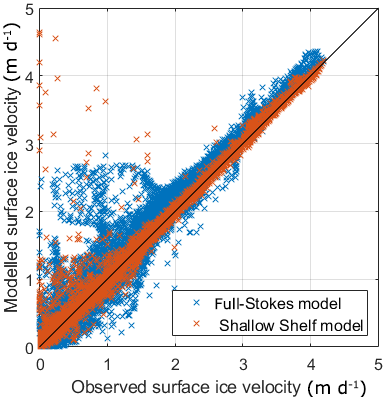
https://www.the-cryosphere.net/14/17/2020/tc-14-17-2020-f06

Figure A1Comparison between observed surface ice velocities, obtained from the MEaSUREs version 2 dataset (Rignot et al., 2017, 2011 b; Mouginot et al., 2012), and modelled ice velocities using either the 3-D model (Sect. 2.1, blue crosses) or the Úa model (red crosses).

Appendix B: Modelling of grounded ice

The main challenge to address when adding grounded ice streams into the RF_streams model domain is to reproduce the correct basal sliding velocity (v_b). We use a Weertman sliding law of the form

\begin{matrix} (B1) & v_{b} = β τ_{b}^{m}, \end{matrix}

where β is basal slipperiness, τ_b is the basal traction and m is a stress exponent. Using an inverted slipperiness field from a shallow shelf model (as we can do for the rate factor on the ice shelf; see Appendix A) is not possible as the difference in the stress regime between the two models can become large on grounded ice and thus yields a velocity field that does not match observations.

We use the inverse Robin approach outlined in Arthern and Gudmundsson (2010) that consists of solving the forward problem once with standard boundary conditions (denoted 𝒩𝒫) and then the slightly modified Dirichlet problem (denoted 𝒟𝒫) in which the stress-free upper-surface condition (Eq. 10) is replaced by a Dirichlet condition where horizontal velocities derived from observations are imposed. The aim of this procedure is to minimise the Kohn and Vogelius cost function:

\begin{matrix} (B2) & J_{kv} = \int_{Γ_{b}} β {|v^{N} - v^{D}|}_{F}^{2} d Γ, \end{matrix}

where v^N and v^D are basal velocities obtained by solving 𝒩𝒫 and 𝒟𝒫, respectively, Γ_b is the basal boundary and ${|.|}_{F}^{2}$ denotes the Frobenius norm. The Gateaux derivative of the cost function 𝒥_KV with respect to the slipperiness β is given by

\begin{matrix} (B3) & d_{β} J_{kv} = \int_{Γ_{b}} β^{'} ({|v^{D}|}_{F}^{2} - {|v^{N}|}_{F}^{2}) d Γ . \end{matrix}

This derivative is strictly only exact for a linear ice rheology; nevertheless, we use it here as an approximation to the true derivative as has been done by previous authors (Arthern and Gudmundsson, 2010; Gillet-Chaulet et al., 2012).

Following Gillet-Chaulet et al. (2012), we make several modifications to the original approach described by Arthern and Gudmundsson (2010). Firstly we apply a change of variables and invert for α=log ₁₀β, which avoids any unphysical negative values appearing during the inversion procedure. This necessitates adding a correction to the gradient given in Eq. (B3) of

\begin{matrix} (B4) & d_{α} J_{kv} = d_{β} J_{kv} \ln (10) β . \end{matrix}

Secondly, because both data and model errors are present, it is necessary to avoid overfitting the model to data, which would lead to spurious changes in slipperiness. To this end, we impose a smoothness constraint on the total cost function by adding a Tikhonov style regularisation term of the form

\begin{matrix} (B5) & J_{reg} = \frac{γ}{2} \int_{Γ_{b}} {|\nabla α|}^{2} d Γ, \end{matrix}

where γ is a parameter that must be carefully chosen to ensure a sensible compromise between a smooth solution and small misfit. We perform an L-curve analysis to determine an optimum value of $γ = 10^{- 3}$ .

In the finite-element-method context, this regularisation term can be easily evaluated given the stiffness matrix, K, such that the regularisation term in Eq. (B5) is given by

\begin{matrix} (B6) & J_{reg} = \frac{γ}{2} α^{T} K α . \end{matrix}

The gradient of this term with respect to α is simply

\begin{matrix} (B7) & d_{α} J_{reg} = γ K α . \end{matrix}

Finally, the total cost function we seek to minimise is $J = J_{kv} + J_{reg}$ with gradient $g = d_{α} J_{kv} + d_{α} J_{reg}$ given by Eqs. (B4) and (B7).

We use the native minimisation algorithm in MATLAB© to minimise 𝒥. Once the inversion procedure has converged to produce a slipperiness field for grounded ice we can use the sliding law in Eq. (B1) as a boundary condition for the grounded parts of the model. The same Dirichlet BC that is used on grounded boundary nodes in the default setup (Eq. 11) is applied to nodes at the boundaries of the newly added ice streams.

Appendix C: Calculation of a damage field

We employ a continuum damage mechanics approach to simulate the effects of damage on ice behaviour. In this framework, the elastic modulus E is pre-multiplied by a damage factor, D, such that $\tilde{E} = E (1 - D)$ , where $\tilde{E}$ is now the effective elastic modulus of damaged ice. The damage factor can be thought of as a measure of the amount of voids in a given unit volume and a high damage factor reduces the portion of a body that can support a load. This simple approach means that in areas of high damage, such as where the ice is heavily crevassed, the effective elastic modulus is reduced and so the ice is less stiff.

We do not allow damage to evolve or advect on the shelf and instead we use the approach of Borstad et al. (2013) to calculate a static damage field. The basic principle of their approach is to take the results of an inversion for the ice rigidity ( $B = A^{1 / n}$ ) and assume that spatial variations in this field arise from variations in temperature, back stress and damage. The damage field is then calculated as

\begin{matrix} (C1) & D = 1 - \frac{B_{i -}}{B (T)}, \end{matrix}

where

\begin{matrix} (C2) & B_{i -} = \{\begin{cases} B_{i} & if B_{i} \leq B (T) . \\ B (T) & otherwise \end{cases} \end{matrix}

B_i is the bulk ice rigidity and B(T) is the ice rigidity that would be expected based purely on its dependence on temperature.

The only missing ingredient in the equations described above is a temperature field of the ice shelf in order to obtain B(T). We use the analytical solution for ice shelf temperature from Holland and Jenkins (1999), which includes both diffusion and vertical advection. The solution assumes that vertical velocity in the ice shelf is equal to the basal melting rate (w_B) and that the ice shelf is in steady state, such that $w = (ρ_{w} / ρ) w_{B}$ . In addition, surface and basal temperatures are needed as boundary conditions for the solution. We obtain the surface temperature field T_S as a yearly average of the snow layer temperature from ERA-Interim (Dee et al., 2011). We then fix temperature at the base of the ice shelf (T_B) at −2 ^∘C. The resulting vertical temperature profile is given by

\begin{matrix} (C3) & T (z) = \frac{(T_{S} - T_{B}) \exp (\frac{- w z}{κ}) + T_{B} - T_{S} \exp (\frac{w h}{κ})}{1 - \exp (\frac{w h}{κ})}, \end{matrix}

where $κ = 1.14 \times 10^{- 6}$ is the ice shelf thermal conductivity. With this temperature field, we calculate the temperature dependent ice rigidity using the relation derived in Smith (1981).

The resulting damage field, as calculated from Eq. (C1), is shown in Fig. C1. An exhaustive assessment of the resulting damage field is beyond the scope of this study, but areas of high damage are identified along shear margins giving some confidence that this calculation yields a sensible result. The damage factor enters the model by altering the modelled elastic behaviour of ice in regions where damage is high through a reduction in the effective elastic modulus, as outlined above.

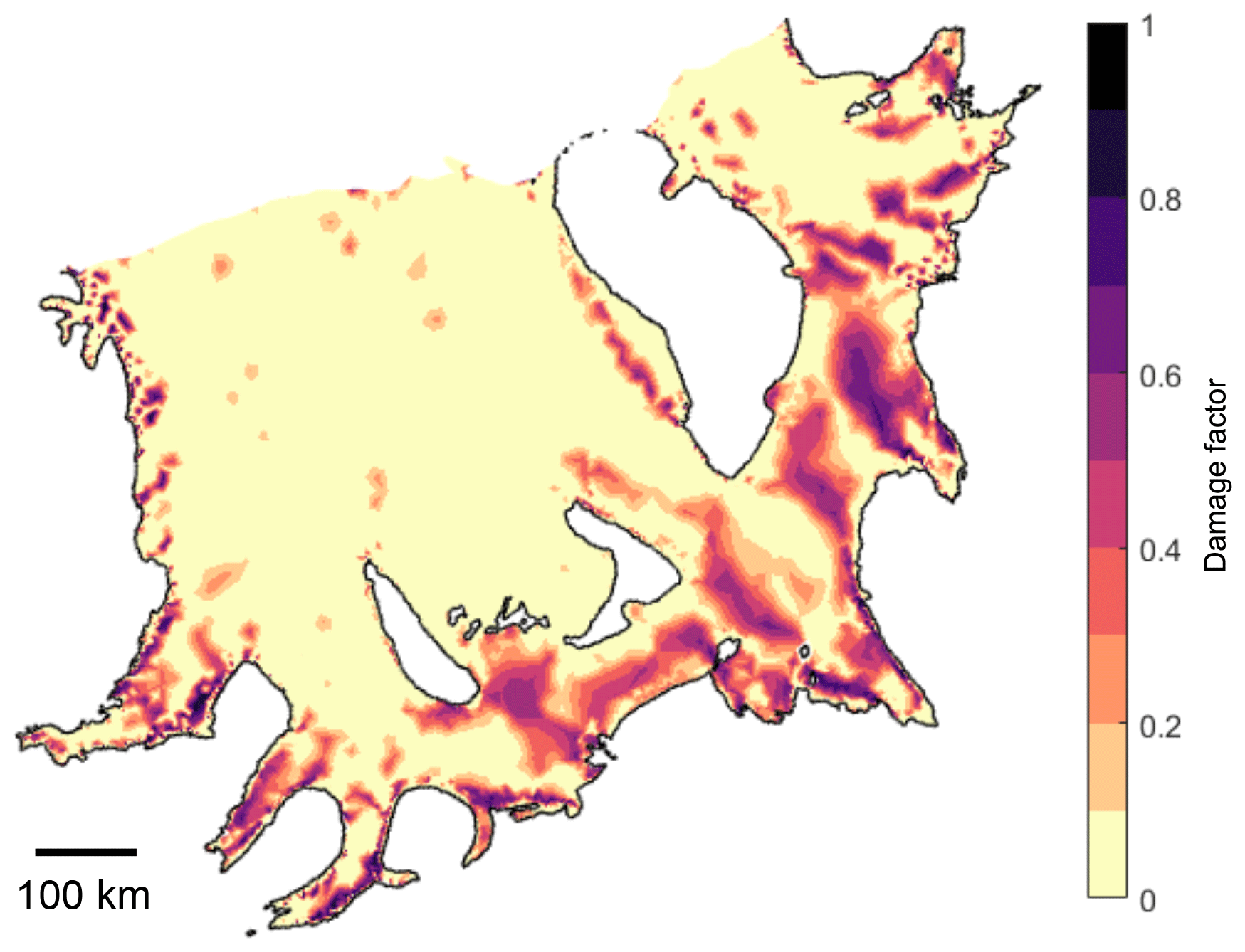
https://www.the-cryosphere.net/14/17/2020/tc-14-17-2020-f07

Figure C1Damage factor field over the Filchner–Ronne Ice Shelf, as calculated with Eq. (C1).

Appendix D: Burgers rheology

The viscoelastic rheological model used in the majority of full Stokes ice flow model experiments to date is the Maxwell model, consisting of a viscous dashpot and elastic spring connected in series (Sect. 2.1). When a stress is applied to a body of ice this rheological model captures both the instantaneous elastic deformation and the long-term viscous response and is one of the simplest representations of viscoelastic behaviour. Another relatively simple rheological representation is given by a Kelvin model, consisting of a viscous dashpot and elastic spring connected in parallel. In this case the model exhibits a delayed elastic response commonly found in many viscoelastic materials and missed in the Maxwell model. The Kelvin model does not, however, capture either instantaneous elastic deformation or long-term viscous behaviour and thus would be of limited use in this modelling framework. A more complex model is needed to capture all of these behaviours and for that purpose we can use a Burgers model, consisting of a Kelvin and Maxwell element connected in series.

The constitutive equation of the Burgers model for deviatoric behaviour is given by

\begin{matrix} (D1) & τ_{i j} + p_{1} {\dot{τ}}_{i j} + p_{2} {\ddot{τ}}_{i j} = q_{1} {\dot{e}}_{i j} + q_{2} {\ddot{e}}_{i j}, \end{matrix}

where

\begin{array}{l} (D2) & p_{1} = \frac{η_{M}}{G_{M}} + \frac{η_{M}}{G_{K}} + \frac{η_{K}}{G_{K}}, \\ (D3) & p_{2} = \frac{η_{K} η_{M}}{G_{K} G_{M}}, \\ (D4) & q_{1} = 2 η_{M}, \end{array}

and

\begin{matrix} (D5) & q_{2} = \frac{2 η_{K} η_{M}}{G_{K}} . \end{matrix}

In the equations set out above, η_M and η_K are the viscosities of the Maxwell and Kelvin elements of the Burgers model, while G_M and G_K are the corresponding shear moduli, related to the Young's Modulus and Poisson's ratio through Eq. (5) (Shames and Cozzarelli, 1997). The volumetric deformation is assumed to be elastic and is defined in terms of the bulk modulus K as

\begin{matrix} (D6) & σ_{i i} = 3 K ε_{i i}, \end{matrix}

where $K = E / 3 (1 - 2 ν)$ . The instantaneous elastic response of the Burgers model is determined by the shear Modulus G_M in the Maxwell element and by the bulk modulus K. The Kelvin element parameters, G_K and η_K, determine the delayed elastic response (primary creep). Finally, the steady-state viscous strain, which is the only behaviour included in most ice shelf models, is determined by the viscosity of the dashpot in the Maxwell element (η_M). Following Gudmundsson (2011) and Reeh et al. (2003), we use the values G_M=3.5 GPa, K=8.9 GPa, G_K=3.3 GPa, and η_K=600 GPa s, and set η_M to the standard effective viscosity used in the Glen–Steinemann flow law. A major disadvantage of using a Burgers rheology is that, due to the short relaxation time of the Kelvin element (of the order of minutes), the model requires very short time steps to accurately model the primary creep behaviour.

Appendix E: Grounding line migration

Calculating tidally induced grounding line migration directly, by solving the contact problem, has been done previously using this model in a 2-D flow line case (Rosier et al., 2014). Solving the contact problem for a high-resolution model of the entire Filchner–Ronne region would be prohibitively expensive computationally. Furthermore, with no detailed information on the bed slope around (and particularly downstream of) grounding lines this approach would still not yield a reliable assessment of grounding line migration. For these reasons, we reject this methodology and instead adopt a simpler approach using the analytical solution for grounding line migration proposed by Tsai and Gudmundsson (2015), which gives upstream and downstream migration distances as $Δ L^{+} = Δ S^{+} / γ^{+}$ and $Δ L^{-} = Δ S^{-} / γ^{-}$ , where

\begin{matrix} (E1) & γ^{+} = β + \frac{ρ}{ρ_{w}} (α - β), \end{matrix}

\begin{matrix} (E2) & γ^{-} = \frac{γ^{+}}{(1 - ρ / ρ_{w})}, \end{matrix}

and $Δ S^{+ / -}$ is a positive or negative vertical tidal motion. These equations assume hydrostatic equilibrium and constant bed (β) and surface (α) slopes. An important result is that, under these assumptions, the upstream migration distance will be greater than the downstream migration distance for a positive or negative tidal deflection of the same amplitude. This analytical solution agreed reasonably well with GL migration calculated by solving the contact problem in the flow line version of this model (Rosier et al., 2014).

Since, as stated above, we have no accurate knowledge of bed slopes in the model domain, we assume that for the purposes of grounding line migration slopes are the same everywhere. This means that the distance the grounding line migrates in the model becomes a function of local tidal amplitude and phase only.

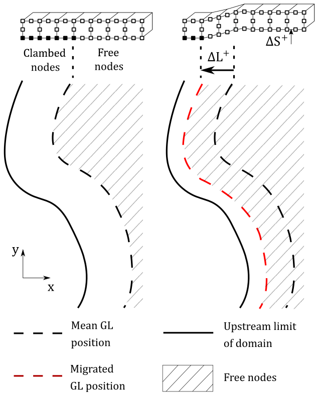
https://www.the-cryosphere.net/14/17/2020/tc-14-17-2020-f08

Figure E1Plan view of a grounding zone, showing how grounding line motion is imposed in the model. Initially the model runs with no tides until it has visco-elastically relaxed. Nodes upstream of the grounding line are clamped at the base and nodes downstream have no constraints. Once tides are switched on, the grounding line can migrate upstream (ΔL⁺) or downstream (ΔL⁻) and nodes that are outside of the defined grounded area have any constraints removed.

Download

Implementing this into the model involves several steps. Firstly we calculate the distance of every node from the default grounding line position as given by Bedmap2, d_GL, where distance is defined as positive for nodes upstream of the grounding line and negative for nodes downstream. Then, given the current local sea surface height, we calculate the current grounding line position using the equations derived by Tsai and Gudmundsson (2015). The basal boundary condition is then applied to nodes along the base of the ice shelf as follows:

\begin{matrix} (E3) & u, v, w = \{\begin{cases} 0 & if Δ L \leq d_{GL} \\ free & otherwise, \end{cases} \end{matrix}

where u, v and w are the nodal displacements. A weakness of this approach is that it cannot be used in a region where ice is flowing rapidly across the grounding line, i.e. at the outlet of major ice streams, since the basal sliding velocity of grounded nodes is set to zero. Therefore, we do not apply this BC in these locations.

A different finite-element mesh is needed for any experiments that include GL migration, since the domain must include a band upstream of the GL which it can migrate into. We add a 10 km band of ice everywhere upstream of GLs except those at the outlet of major ice streams. Mesh resolution in this band is ∼ 500 m to resolve GL motion as accurately as possible without creating an excessively large number of additional elements. A schematic showing how grounding line migration is implemented in our finite-element model is shown in Fig. E1.

Appendix F: Sub-ice-shelf currents

In order to simulate the effect of tidal current drag on the ice shelf, we use the depth-averaged tidal currents from the CATS2008a model (Padman et al., 2002). This provides amplitude and phase of the U and V components of tidal current transport for each of the four major tidal constituents beneath the shelf (M₂, S₂, O₁ and K₁). Following Robertson et al. (1985) and Brunt and MacAyeal (2014), the x and y components of basal shear stress (τ_x and τ_y, respectively) resulting from tidal currents are defined as

\begin{matrix} (F1) & \begin{aligned} τ_{x} = \frac{C_{D} ρ_{w} U |U_{T}|}{H^{2}}, \\ τ_{y} = \frac{C_{D} ρ_{w} V |U_{T}|}{H^{2}}, \end{aligned} \end{matrix}

where H is water column thickness, C_D is the drag coefficient and $U_{T} = \sqrt{U^{2} + V^{2}}$ is the magnitude of the tidal current transport vector. The drag coefficient is an unknown related to the roughness of the ice shelf base. We investigated two choices for C_D, a typical value of 0.003 (Robertson et al., 1985; Brunt and MacAyeal, 2014) and a much higher value of 0.03 which we use to test a theoretical upper limit on tidal current effects. The basal shear stresses are applied directly to the bottom face of the ice shelf elements at the same time as vertical tides are initiated within the model.

Appendix G: Temperature effects

The effects of temperature on ice rheology are, to a certain extent, included in every version of the model; since a part of the spatial variation in the inverted rate factor field is caused by temperature. One aspect of temperature variations that is not included, however, is the change in temperature with depth. This will result in ice that deforms more easily at the base than at the surface, since ice will generally be cooler at the surface and warmer at the ice shelf base. This could conceivably play an important role in the response of an ice shelf to tides and is particularly relevant for the tidal flexure mechanism since here it is the ice rheology that is the source of non-linearity that we seek to reproduce.

We are specifically interested in the effects of depth variation in ice softness and to explore this in the simplest way possible we assume that, everywhere in the ice shelf, temperature varies linearly from −20 ^∘C at the surface to −2 ^∘C at the base. We then make the rate factor a function of temperature using the relation derived by Smith (1981).

Appendix H: Thin grounding zone experiment

Ice thickness within the grounding zone (GZ) is modified in the RF_thinGZ experiment to explore how this might affect generation of the M_sf signal, in particular by changing flexural stresses resulting from tidal bending. The crude approach that we take for a first-order estimate of this affect is to multiply ice thickness h by a factor 1−λ that is a function of distance from the grounding line (d_GL), defined such that at the grounding line and far away from the grounding zone λ=0 but within the grounding zone $0 < λ < 1$ . The arbitrary function that we choose for this purpose is a log-normal distribution centred around d_GL=1 km, where it reaches a maximum value of 0.1, i.e. leading a maximum reduction in ice thickness of 10 %. Multiplying ice thickness by this factor yields a new ice thickness field that retains its overall shape and the effect is confined such that $λ \approx 1 \times 10^{- 2}$ at d_GL=10 km and $λ \approx 1 \times 10^{- 3}$ at d_GL=20 km (beyond this distance from the grounding line we do not alter ice thickness).

Data availability

The GPS dataset that was analysed to determine horizontal tidal displacement of the Ronne Ice Shelf is publicly available through the UK Polar Data Centre at https://doi.org/10.5285/4fe11286-0e53-4a03-854c-a79a44d1e356 (Gudmundsson et al., 2017 b), and the analysis of that dataset is carried out in Rosier et al. (2017 a).

Author contributions

SHRR and GHG conceived the study. SHRR performed the model simulations and prepared the figures and paper draft. SHRR and GHG reviewed and edited the paper.

Competing interests

The authors declare that they have no conflict of interest.

Acknowledgements

We are very grateful to Andrew Bell for his invaluable help with MSC Marc. Sebastian H. R. Rosier was funded by the UK Natural Environment Research Council large grant “Ice shelves in a warming world: Filchner Ice Shelf System” (NE/L013770/1). We also greatly appreciate the work of the editor, Julia Christmann and an anonymous reviewer for their helpful suggestions.

Financial support

This research was funded by the UK Natural Environment Research Council large grant “Ice shelves in a warming world: Filchner Ice Shelf System” (NE/L013770/1).

Review statement

This paper was edited by Evgeny A. Podolskiy and reviewed by Julia Christmann and one anonymous referee.

References

Alley, S. A. R. B.: Tidal forcing of basal seismicity of ice stream C, West Antarctica, observed far inland, J. Geophys. Res., 102, 15813–15196, https://doi.org/10.1029/97JB01073, 1997. a

Anandakrishnan, S., Voigt, D. E., and Alley, R. B.: Ice stream D flow speed is strongly modulated by the tide beneath the Ross Ice Shelf, Geophys. Res. Lett., 30, 1361, https://doi.org/10.1029/2002GL016329, 2003. a

Arthern, R. J. and Gudmundsson, G. H.: Initialization of ice-sheet forecasts viewed as an inverse Robin problem, J. Glaciol., 56, 527–533, https://doi.org/10.3189/002214310792447699, 2010. a, b, c

Bindschadler, R. A., King, M. A., Alley, R. B., Anandakrishnan, S., and Padman, L.: Tidally controlled stick-slip discharge of a West Antasrctic ice stream, Science, 301, 1087–1089, https://doi.org/10.1126/science.1087231, 2003. a

Borstad, C. P., Rignot, E., Mouginot, J., and Schodlok, M. P.: Creep deformation and buttressing capacity of damaged ice shelves: theory and application to Larsen C ice shelf, The Cryosphere, 7, 1931–1947, https://doi.org/10.5194/tc-7-1931-2013, 2013. a

Brunt, K. M. and MacAyeal, D. R.: Tidal modulation of ice-shelf flow: a viscous model of the Ross Ice Shelf, J. Glaciol., 60, 500–508, https://doi.org/10.3189/2014JoG13J203, 2014. a, b, c, d, e, f

Brunt, K. M., King, M. A., Fricker, H. A., and Macayeal, D. R.: Flow of the Ross Ice Shelf , Antarctica, is modulated by the ocean tide, J. Glaciol., 56, 2005–2009, 2010. a, b

Brunt, K. M., Fricker, H. A., and Padman, L.: Analysis of ice plains of the Filchner-Ronne Ice Shelf, Antarctica, using ICESat laser altimetry, J. Glaciol., 57, 965–975, 2011. a, b, c

Codiga, D. L.: Unified Tidal Analysis and Prediction Using the UTide Matlab Functions, Tech. rep., Graduate School of Oceanography, University of Rhode Island, Narragansett, RI, 2011. a

Cuffey, K. M. and Paterson, W. S. B.: The physics of glaciers 4th edn., Elsevier, Amsterdam, 2010. a

De Angelis, H. and Skvarca, P.: Glacier Surge After Ice Shelf Collapse, Science, 299, 1560–1562, https://doi.org/10.1126/science.1077987, 2003. a

Dee, D. P., Uppala, S. M., Simmons, A. J., Berrisford, P., Poli, P., Kobayashi, S., Andrae, U., Balmaseda, M. A., Balsamo, G., Bauer, P., Bechtold, P., Beljaars, A. C. M., van de Berg, L., Bidlot, J., Bormann, N., Delsol, C., Dragani, R., Fuentes, M., Geer, A. J., Haimberger, L., Healy, S. B., Hersbach, H., Hólm, E. V., Isaksen, L., Kållberg, P., Köhler, M., Matricardi, M., McNally, A. P., Monge-Sanz, B. M., Morcrette, J.-J., Park, B.-K., Peubey, C., de Rosnay, P., Tavolato, C., Thépaut, J.-N., and Vitart, F.: The ERA-Interim reanalysis: configuration and performance of the data assimilation system, Q. J. Roy. Meteor. Soc., 137, 553–597, https://doi.org/10.1002/qj.828, 2011. a

Doake, C., Corr, H. F. J., Nicholls, K. W., Gaffikin, A., Jenkins, A., Bertiger, W. I., and King, M. A.: Tide-induced lateral movement of Brunt Ice Shelf , Antarctica, Geophys. Res. Lett., 29, 1–4, https://doi.org/10.1029/2001GL014606, 2002. a, b, c, d, e

Engwirda, D.: Locally-optimal Delaunay-refinement and optimisation-based mesh generation, PhD thesis, School of Mathematics and Statistics, University of Sydney, 2014. a

Fretwell, P., Pritchard, H. D., Vaughan, D. G., Bamber, J. L., Barrand, N. E., Bell, R., Bianchi, C., Bingham, R. G., Blankenship, D. D., Casassa, G., Catania, G., Callens, D., Conway, H., Cook, A. J., Corr, H. F. J., Damaske, D., Damm, V., Ferraccioli, F., Forsberg, R., Fujita, S., Gim, Y., Gogineni, P., Griggs, J. A., Hindmarsh, R. C. A., Holmlund, P., Holt, J. W., Jacobel, R. W., Jenkins, A., Jokat, W., Jordan, T., King, E. C., Kohler, J., Krabill, W., Riger-Kusk, M., Langley, K. A., Leitchenkov, G., Leuschen, C., Luyendyk, B. P., Matsuoka, K., Mouginot, J., Nitsche, F. O., Nogi, Y., Nost, O. A., Popov, S. V., Rignot, E., Rippin, D. M., Rivera, A., Roberts, J., Ross, N., Siegert, M. J., Smith, A. M., Steinhage, D., Studinger, M., Sun, B., Tinto, B. K., Welch, B. C., Wilson, D., Young, D. A., Xiangbin, C., and Zirizzotti, A.: Bedmap2: improved ice bed, surface and thickness datasets for Antarctica, The Cryosphere, 7, 375–393, https://doi.org/10.5194/tc-7-375-2013, 2013. a

Furst, J. J., Durand, G., Gillet-Chaullet, F., Tavard, L., Rankl, M., Braun, M., and Gagliardini, O.: The safety band of Antarctic ice shelves, Nat. Clim. Change, 6, 479–482, https://doi.org/10.1038/nclimate2912, 2018. a

Gillet-Chaulet, F., Gagliardini, O., Seddik, H., Nodet, M., Durand, G., Ritz, C., Zwinger, T., Greve, R., and Vaughan, D. G.: Greenland ice sheet contribution to sea-level rise from a new-generation ice-sheet model, The Cryosphere, 6, 1561–1576, https://doi.org/10.5194/tc-6-1561-2012, 2012. a, b

Glen, J. W.: The creep of polycrystalline ice, Proc. R. Soc. Lon. Ser.-A, 228, 519–538, https://doi.org/10.1098/rspa.1955.0066, 1955. a

Gudmundsson, G. H.: Fortnightly variations in the flow velocity of Rutford Ice Stream, West Antarctica., Nature, 444, 1063–1064, https://doi.org/10.1038/nature05430, 2006. a, b, c

Gudmundsson, G. H.: Tides and the flow of Rutford Ice Stream, West Antarctica, J. Geophys. Res., 112, F04007, https://doi.org/10.1029/2006JF000731, 2007. a, b, c, d

Gudmundsson, G. H.: Ice-stream response to ocean tides and the form of the basal sliding law, The Cryosphere, 5, 259–270, https://doi.org/10.5194/tc-5-259-2011, 2011. a, b, c, d, e, f

Gudmundsson, G. H.: Ice-shelf buttressing and the stability of marine ice sheets, The Cryosphere, 7, 647–655, https://doi.org/10.5194/tc-7-647-2013, 2013. a

Gudmundsson, G. H., Krug, J., Durand, G., Favier, L., and Gagliardini, O.: The stability of grounding lines on retrograde slopes, The Cryosphere, 6, 1497–1505, https://doi.org/10.5194/tc-6-1497-2012, 2012. a, b

Gudmundsson, G. H., De Rydt, J., and Nagler, T.: Five decades of strong temporal variability in the flow of Brunt Ice Shelf, Antarctica, J. Glaciol., 63, 164–175, https://doi.org/10.1017/jog.2016.132, 2017a. a, b

Gudmundsson, G. H., Fenney, N., and Rosier, S. H. R.: Timeseries from GPS units deployed on ice streams and the adjoining ice shelf across the Filchner-Ronne region, Antarctica, 2005–2016, NERC UK Polar Data Centre, https://doi.org/10.5285/4fe11286-0e53-4a03-854c-a79a44d1e356 (last access: 1 February 2019), 2017b. a

Haseloff, M. and Sergienko, O. V.: The effect of buttressing on grounding line dynamics, J. Glaciol., 64, 417–431, https://doi.org/10.1017/jog.2018.30, 2018. a

Holland, D. M. and Jenkins, A.: Modeling Thermodynamic Ice–Ocean Interactions at the Base of an Ice Shelf, J. Phys. Oceanogr., 29, 1787–1800, https://doi.org/10.1175/1520-0485, 1999. a

Hughes, T.: Is the west Antarctic Ice Sheet disintegrating?, J. Geophys. Res., 78, 7884–7910, https://doi.org/10.1029/JC078i033p07884, 1973. a

Hulbe, C. L., Klinger, M., Masterson, M., Catania, G., Cruikshank, K., and Bugni, A.: Tidal bending and strand cracks at the Kamb Ice Stream grounding line, West Antarctica, J. Glaciol., 62, 816–824, https://doi.org/10.1017/jog.2016.74, 2016. a

Hutter, K.: Theoretical Glaciology: Material Science of Ice and the Mechanics of Glaciers and Ice Sheets, Mathematical Approaches to Geophysics, Springer, 1983. a

Jellinek, H. H. G. and Brill, R.: Viscoelastic Properties of Ice, J. Appl. Phys., 27, 1198–1209, https://doi.org/10.1063/1.1722231, 1956. a

King, M. A., Makinson, K., and Gudmundsson, G. H.: Nonlinear interaction between ocean tides and the Larsen C Ice Shelf system, Geophys. Res. Lett., 38, L08501, https://doi.org/10.1029/2011GL046680, 2011. a, b, c, d

Kobarg, W.: The tide-dependent dynamics of the Ekström Ice Shelf, Antarctica, Berichte zur Polarforschung, Alfred-Wegener-Inst. für Polar- u. Meeresforsch., 1988. a

Legresy, B., Wendt, A., Tabacco, I., Remy, F., and Dietrich, R.: Influence of tides and tidal current on Mertz Glacier, Antarctica, J. Glaciol., 50, 427–435, https://doi.org/10.3189/172756504781829828, 2004. a, b, c, d, e

Lingle, C. S., Hughes, T. J., and Kollmeyer, R. C.: Tidal flexure of Jakobshavns Glacier, west Greenland, J. Geophys. Res.-Sol. Ea., 86, 3960–3968, https://doi.org/10.1029/JB086iB05p03960, 1981. a

MacAyeal, D. R.: Large-scale ice flow over a viscous basal sediment: Theory and application to ice stream B, Antarctica, J. Geophys. Res.-Sol. Ea., 94, 4071–4087, https://doi.org/10.1029/JB094iB04p04071, 1989. a

MacAyeal, D. R.: The basal stress distribution of Ice Stream E, Antarctica, inferred by control methods, J. Geophys. Res.-Sol. Ea., 97, 595–603, https://doi.org/10.1029/91JB02454, 1992. a

MacAyeal, D. R.: A tutorial on the use of control methods in ice-sheet modeling, J. Glaciol., 39, 91–98, https://doi.org/10.3189/S0022143000015744, 1993. a

Makinson, K., King, M. A., Nicholls, K. W., and Gudmundsson, G. H.: Diurnal and semidiurnal tide-induced lateral movement of Ronne Ice Shelf, Antarctica, Geophys. Res. Lett., 39, L10501, https://doi.org/10.1029/2012GL051636, 2012. a, b, c, d, e, f, g, h

Marsh, O. J., Rack, W., Floricioiu, D., Golledge, N. R., and Lawson, W.: Tidally induced velocity variations of the Beardmore Glacier, Antarctica, and their representation in satellite measurements of ice velocity, The Cryosphere, 7, 1375–1384, https://doi.org/10.5194/tc-7-1375-2013, 2013. a

Milillo, P., Rignot, E., Mouginot, J., Scheuchl, B., Morlighem, M., Li, X., and Salzer, J. T.: On the Short-term Grounding Zone Dynamics of Pine Island Glacier, West Antarctica, Observed With COSMO-SkyMed Interferometric Data, Geophys. Res. Lett., 44, 10436–10444, https://doi.org/10.1002/2017GL074320, 2017. a, b

Minchew, B. M., Simons, M., Riel, B., and Milillo, P.: Tidally induced variations in vertical and horizontal motion on Rutford Ice Stream, West Antarctica, inferred from remotely sensed observations, J. Geophys. Res.-Earth, 122, 167–190, https://doi.org/10.1002/2016JF003971, 2016. a, b, c, d, e, f, g, h

Minowa, M., Podolskiy, E. A., and Sugiyama, S.: Tide-modulated ice motion and seismicity of a floating glacier tongue in East Antarctica, Ann. Glaciol., 60, 57–67, https://doi.org/10.1017/aog.2019.25, 2019. a

Mouginot, J., Scheuchl, B., and Rignot, E.: Mapping of Ice Motion in Antarctica Using Synthetic-Aperture Radar Data, Remote Sensing, 4, 2753–2767, https://doi.org/10.3390/rs4092753, 2012. a, b, c

MSC: Marc 2017 Volume A: Theory and user information, MSC MARC, MSC Software Corporation, 2 MacArther Place, Santa Ana, CA 92707, 2017. a

Padman, L., Fricker, H. A., Coleman, R., Howard, S., and Erofeeva, S. Y.: A new tide model for the Antarctic ice shelves and seas, Ann. Glaciol., 34, 247–254, 2002. a, b, c, d

Pegler, S. S.: Marine ice sheet dynamics: the impacts of ice-shelf buttressing, J. Fluid Mech., 857, 605–647, https://doi.org/10.1017/jfm.2018.741, 2018. a

Pirli, M., Hainzl, S., Schweitzer, J., Köhler, A., and Dahm, T.: Localised thickening and grounding of an Antarctic ice shelf from tidal triggering and sizing of cryoseismicity, Earth Planet. Sc. Lett., 503, 78–87, https://doi.org/10.1016/j.epsl.2018.09.024, 2018. a

Rack, W., King, M. A., Marsh, O. J., Wild, C. T., and Floricioiu, D.: Analysis of ice shelf flexure and its InSAR representation in the grounding zone of the southern McMurdo Ice Shelf, The Cryosphere, 11, 2481–2490, https://doi.org/10.5194/tc-11-2481-2017, 2017. a

Reeh, N., Christensen, E. L., Mayer, C., and Olesen, O. B.: Tidal bending of glaciers: a linear viscoelastic approach, Ann. Glaciol., 37, 83–89, https://doi.org/10.3189/172756403781815663, 2003. a

Reese, R., Gudmundsson, G. H., Levermann, A., and Winkelmann, R.: The far reach of ice-shelf thinning in Antarctica, Nat. Clim. Change, 8, 53–57, https://doi.org/10.1038/s41558-017-0020-x, 2018. a

Riedel, B., Nixdorf, U., Heinert, M., Eckstaller, A., and Mayer, C.: The response of the Ekstromisen (Antarctica) grounding zone to tidal forcing, Ann. Glaciol., 29, 239–242, https://doi.org/10.3189/172756499781821247, 1999. a, b

Rignot, E., Casassa, G., Gogineni, P., Krabill, W., Rivera, A., and Thomas, R.: Accelerated ice discharge from the Antarctic Peninsula following the collapse of Larsen B ice shelf, Geophys. Res. Lett., 31, L18401, https://doi.org/10.1029/2004GL020697, 2004. a

Rignot, E., Mouginot, J., and Scheuchl, B.: Ice Flow of the Antarctic Ice Sheet, Science, 333, 1427–1430, https://doi.org/10.1126/science.1208336, 2011a. a, b

Rignot, E. J., Mouginot, J., and Scheuchl, B.: Antarctic grounding line mapping from differential satellite radar interferometry, Geophys. Res. Lett., 38, L10504, https://doi.org/10.1029/2011GL047109, 2011b. a

Rignot, E., Mouginot, J., and Scheuchl, B.: MEaSUREs InSAR-Based Antarctica Ice Velocity Map, Version 2, https://doi.org/10.5067/D7GK8F5J8M8R, 2017. a, b, c

Robel, A. A., Tsai, V. C., Minchew, B., and Simons, M.: Tidal modulation of ice shelf buttressing stresses, Ann. Glaciol., 58, 12–20, https://doi.org/10.1017/aog.2017.22, 2017. a, b, c

Robertson, R., Padman, L., and Egbert, G. D.: Tides in the Weddell Sea, American Geophysical Union (AGU), 341–369, https://doi.org/10.1029/AR075p0341, 1985. a, b

Rosier, S. H. R. and Gudmundsson, G. H.: Tidal bending of ice shelves as a mechanism for large-scale temporal variations in ice flow, The Cryosphere, 12, 1699–1713, https://doi.org/10.5194/tc-12-1699-2018, 2018. a, b, c, d, e

Rosier, S. H. R., Gudmundsson, G. H., and Green, J. A. M.: Insights into ice stream dynamics through modelling their response to tidal forcing, The Cryosphere, 8, 1763–1775, https://doi.org/10.5194/tc-8-1763-2014, 2014. a, b, c, d, e, f, g

Rosier, S. H. R., Gudmundsson, G. H., and Green, J. A. M.: Temporal variations in the flow of a large Antarctic ice stream controlled by tidally induced changes in the subglacial water system, The Cryosphere, 9, 1649–1661, https://doi.org/10.5194/tc-9-1649-2015, 2015. a, b

Rosier, S. H. R., Gudmundsson, G. H., King, M. A., Nicholls, K. W., Makinson, K., and Corr, H. F. J.: Strong tidal variations in ice flow observed across the entire Ronne Ice Shelf and adjoining ice streams, Earth Syst. Sci. Data, 9, 849–860, https://doi.org/10.5194/essd-9-849-2017, 2017a. a, b, c, d, e, f, g, h, i

Rosier, S. H. R., Marsh, O. J., Rack, W., Gudmundsson, G. H., Wild, C. T., and Ryan, M.: On the interpretation of ice-shelf flexure measurements, J. Glaciol., 63, 783–791, https://doi.org/10.1017/jog.2017.44, 2017b. a

Rott, H., Rack, W., Skvarca, P., and Angelis, H. D.: Northern Larsen Ice Shelf, Antarctica: further retreat after collapse, Ann. Glaciol., 34, 277–282, https://doi.org/10.3189/172756402781817716, 2002. a

Schmeltz, M., Rignot, E., and MacAyeal, D. R.: Ephemeral grounding as a signal of ice-shelf change, J. Glaciol., 47, 71–77, https://doi.org/10.3189/172756501781832502, 2001. a, b

Schmeltz, M., Rignot, E. J., and MacAyeal, D.: Tidal flexure along ice-sheet margins: comparison of InSAR with an elastic-plate model, Ann. Glaciol., 34, 202–208, https://doi.org/10.3189/172756402781818049, 2002. a

Shames, I. H. and Cozzarelli, F. A.: Elastic and Inelastic Stress Analysis, Taylor and Francis, 325 CHestnut St., Philadelphia, 19106, 1997. a, b, c

Smith, A. M.: The use of tiltmeters to study the dynamics of Antarctic ice-shelf grounding lines, J. Glaciol., 37, 51–58, 1991. a

Smith, G. D.: Viscous relations for the steady creep of polycrystalline ice, Cold Reg. Sci. Technol., 5, 141–150, 1981. a, b

Steinemann, S.: Results of Preliminary Experiments on the Plasticity of Ice Crystals, J. Glaciol., 2, 404–416, https://doi.org/10.3189/002214354793702533, 1954. a

Stephenson, S. N.: Glacier flexure and the position of grounding lines: Measurements by tiltmeter on Rutford Ice Stream Antarctica, Ann. Glaciol., 5, 165–169, 1984. a

Sykes, H. J., Murray, T., and Luckman, A.: The location of the grounding zone of Evans Ice Stream, Antarctica, investigated using SAR interferometry and modelling, Ann. Glaciol., 50, 35–40, https://doi.org/10.3189/172756409789624292, 2009. a

Thomas, R. H.: The Creep of Ice Shelves: Interpretation of Observed Behaviour, J. Glaciol., 12, 55–70, https://doi.org/10.3189/S002214300002270X, 1973. a

Thompson, J., Simons, M., and Tsai, V. C.: Modeling the elastic transmission of tidal stresses to great distances inland in channelized ice streams, The Cryosphere, 8, 2007–2029, https://doi.org/10.5194/tc-8-2007-2014, 2014. a

Tsai, V. C. and Gudmundsson, G. H.: An improved model for tidally-modulated grounding line migration, J. Glaciol., 61, 216–222, https://doi.org/10.3189/2015JoG14J152, 2015. a, b, c, d, e

Vaughan, D. G.: Tidal flexure at ice shelf margins, J. Geophys. Res., 100, 6213–6224, 1995. a

Exploring mechanisms responsible for tidal modulation in flow of the Filchner–Ronne Ice Shelf

1.1 Ocean tides beneath the Filchner–Ronne Ice Shelf

1.2 Observations of tidally modulated horizontal ice shelf displacement

1.3 Proposed mechanisms for tidal modulation of ice shelf flow

2.1 Field equations

2.2 Boundary conditions

2.3 Tidal forcing

2.4 Element discretisation

3.1 Semidiurnal (M2) results

3.2 Lunar synodic fortnightly (Msf) results

3.2.1 Flexural softening experiments

3.2.2 Grounding line migration experiments

3.1 Semidiurnal (M₂) results

3.2 Lunar synodic fortnightly (M_sf) results