

Abstract
The equilibrium of pregnant women is compromised because the falling risk increases as pregnancy progresses. The trajectories of the centers of pressure are related to equilibrium, gait and posture. The purpose of this work was to investigate the fractal behavior of the trajectories of the center of pressure of both feet in standing and walking pregnant women and how they evolve during pregnancy. By using instrumented insoles (F-Scan® system working at 40 Hz), the trajectories of the center of pressure of both feet were obtained for 71 women in the three trimesters of their pregnancy. The 'detrended fluctuation analysis', a technique designed to extract the fractal properties of a signal, was used to analyze the fractal behavior of both the x and y components of the measured trajectories. Specifically, the fractal characteristic exponents corresponding to the small and large end regions of the corresponding scaling functions were obtained and compared. No differences were found between the characteristic exponents obtained for x and y components nor from the signals found for left and right feet within the statistical uncertainties. In standing conditions all the exponents obtained remained almost constant, regardless of the elapsed pregnancy time, taking values around 0.5. In walking conditions, the small end exponents did not change with respect to those found in static conditions; on the contrary, the large-end exponents reduced as pregnancy progressed, reaching values of the order of −0.6 in the third trimester. The multi-scaling character of the walking signals could be related to the anteroposterior and medio-lateral displacement observed in previous experiments and that could be on the root of the development of musculoskeletal discomfort and a falling risk that increases with the pregnancy time.
Export citation and abstract BibTeX RIS
1. Introduction
Pregnancy produces significant variations in the gait and postural sway, with increasing falling risk as it progresses. To counteract this risk, pregnant women activate mechanisms in which the forefoot loads are enhanced with respect to the rearfoot ones and this has been indicated as a source of possible musculoskeletal discomfort (Ribeiro et al 2013). The changes in the way the feet rest on the ground produce modifications in the plantar center of pressure (CoP) trajectories and relatively large displacements, with respect to non-pregnant women, were observed in both anteroposterior and medio-lateral directions, mainly in the last trimester of pregnancy (Nyska et al 1997, Ribas and Guirro 2007, Karadag-Saygi et al 2010, Zhang et al 2015, Mei et al 2018).
Plantar CoP trajectories in various situations have been investigated by using instrumented insoles (Winter 1995, Chesnin et al 2000, Martínez-Martí et al 2014, 2016). These devices permit to monitor the movement of both left and right foot plantar CoPs when the subject is either standing or walking. In addition, many others variables related to gait, such as the time support or the position of the foot in swing phase, may be also measured.
The purpose of the present work was to analyze the evolution during pregnancy of the plantar CoP trajectories of pregnant women obtained with instrumented insoles. Instead of the statistical properties of the CoP paths, such as the area enclosing the CoP or the length of the total CoP excursion, already analyzed (Nyska et al 1997, Ribas and Guirro 2007, Karadag-Saygi et al 2010, Ribeiro et al 2013, Zhang et al 2015, Mei et al 2018), we concentrated here on the fractal, non-stationary time characteristics of the CoP trajectories.
To do that, the so-called 'detrended fluctuation analysis' (DFA) technique was used. The DFA method was introduced by Peng et al (1994) and has been considered in many different contexts (Peng et al 1995, Eke et al 2002, Blázquez et al 2009). To characterize the signals analyzed, it uses a scaling exponent that is linked to their fractal behavior.
The procedure we have followed is similar to that considered in previous works to study CoP paths corresponding to the whole body and obtained by means of force platforms (Duarte and Zatsiorsky 2001, Delignières et al 2003, Blázquez et al 2012).
2. Material and methods
2.1. Instrumented Insoles
In this work, the data corresponding to the plantar CoPs were obtained by using F-Scan® (TekScan, Boston, USA), a commercial system that includes two instrumented insoles and a datalogger unit that is situated in the lower back of the subject (Tekscan 2018). This system provides dynamic pressure, force and timing information such as the CoP position and trajectories during standing or walking phases, allowing a complete and detailed gait analysis.
The insoles are made of a flexible plastic substrate which contains up to 954 resistive sensing elements that are organized as a set of rows and columns (Tekscan 2018). Their width is 2.5 mm and they are spaced by 5.1 mm, which means a total of 60 rows and 21 columns. The insoles are laminated on both sides with a 0.1 mm flexible protective covering, and the total thickness in sensing region is 0.15 mm. Pressure range goes from 517 to 862 kPa. Insoles are inserted into a sport shoe provided by the research group, and then connected to the datalogger. Data are sent to the computer through a Wi-Fi connection.
The coordinates of the instantaneous position of the plantar CoP were calculated as (Chesnin et al 2000):
where pi is the pressure measured by the i-th sensor in the insoles and (xi, yi) are the coordinates of its center. In our experiment a sampling frequency of 40 Hz was chosen. Given the huge number of sensors per foot in the F-Scan® system and the definition of the plantar CoP coordinates, we consider that this frequency is enough for this study. Moreover, results can be directly compared with the results of previous works in which data were collected with the same acquisition frequency to study postural sway using a force platform (Duarte and Zatsiorsky 2001, Delignières et al 2003, Blázquez et al 2009, 2010, 2012).
2.2. Characteristics of the subject sample
In the present work we have analyzed the plantar CoP trajectories of both feet in standing and walking pregnant. A total of 71 women participated in the experiment. Table 1 shows the average and range values of the age, height and weight of the women included in the sample studied. The weight data are given for the three trimesters.
Table 1. Data of the women included in the sample analyzed in the present work. The average and standard deviation and the value range are given for the age, height and weight, this last in each of the three pregnancy trimesters.
| average | range | |
|---|---|---|
| age (year) | 31.3 ± 4.7 | [17.0–41.0] |
| height (cm) | 163.2 ± 7.4 | [150.0–183.0] |
| weight 1st. trimester (kg) | 64.1 ± 11.9 | [43.0–106.0] |
| weight 2nd. trimester (kg) | 70.0 ± 11.7 | [53.0–111.0] |
| weight 3rd. trimester (kg) | 76.1 ± 12.7 | [56.0–123.0] |
According to the results shown in table 1, the average values, standard deviations and ranges concerning the weight of the women participating in the study were statistically compatible, but differences in the individual weight gain throughout pregnancy were not analyzed in this work and were not used as an exclusion criterium for participation.
Data in standing and walking conditions were obtained for the women participating in the experiment. Specifically, the instrumented insoles permitted us to obtain the plantar CoP trajectories of both feet. These trajectories provide the evolution with time of the CoP position in a given system of reference. From each one of the plantar CoP trajectories, two signals corresponding to the x (medio-lateral) and the y (anteroposterior) coordinates were extracted. As a result, each dataset consisted of four signals, corresponding to the left and right feet, x and y directions. Measurements were taken in the first (∼12th week), second (∼20th week), and third (∼32nd week) trimesters of pregnancy. The number of datasets obtained in our experiment is summarized in table 2. Different reasons made impossible having the complete information, including the 24 signals above indicated, for all the women included in the study. In much of these cases women agreed to participate after the first pregnancy trimester and some of them did not attended the last measuring period. Summarizing, we had the complete information only for 42 out of the 71 women in the sample. In any case the analysis was done for all the signals available.
Table 2. Number of signals available for the standing and walking women in each of the three pregnancy trimesters. The length range of the signals available, given in terms of their number of points, are also shown.
| standing | walking | |||
|---|---|---|---|---|
| # of datasets | # of points | # of datasets | # of points | |
| 1st. trimester | 54 | [149–3028] | 55 | [248–1924] |
| 2nd. trimester | 65 | [218–2546] | 67 | [441–2460] |
| 3rd. trimester | 62 | [243–1206] | 60 | [642–3610] |
In the experimental procedure, women were asked to stand for a few seconds and then walk as comfortably as possible, at the speed they wanted. That is, measurements were carried out without precise time pattern and, as a consequence, the lengths of the signals measured varied. The shortest signal, with 149 points, was that of subject #33, standing, at the 1st. trimester; the largest one corresponded to subject #62, walking, at the 3rd. trimester, with 3610 points. In general there was no correlation between the lengths of the standing and walking signals for any patient.
The study protocol was approved by the ethics committee of the hospital where measurements were carried out. All the women signed the informed consent for participating and the ethical principles enunciated in the Declaration of Helsinki were taken into account in the measurement procedure.
2.3. The detrended fluctuation analysis method
In the present work, the DFA method has been used to investigate the correlation properties of the plantar CoP trajectories obtained as indicated above. The fractal scaling exponents that characterize the signals in this method are calculated as follows.
Let {ξ} ≡ {ξi = ξ(ti); i = 1, 2, ..., M} be the original series whose data are assumed to be measured with a fixed frequency. The first step is to calculate a new series, {Θ} ≡ {Θl; l = 1, 2, ..., M}, whose elements are

It is simply the accumulated series referred to the average of the M data of the original series, which is given by:

Now, a set of p subseries labelled as  are extracted from the accumulated series {Θ}. These p pieces span the whole series {Θ}, may overlap each other or not, and all of them contain τ consecutive values:

A polynomial of degree q,  , is fitted to each one the pieces
  and the series

is calculated. Here

and lm indicates the initial point of the corresponding subseries that depends on the index m.  is the so-called detrended fluctuation series and is obtained once the local trend of the signal, which is represented by the fitting polynomial, is substracted from the subseries
  .
.
Finally, the important quantity is the root mean squared fluctuation of the subseries with size τ:

The original signal is said to show scaling properties if F(τ) ∼ τα. In that case, the scaling exponent α determines the fractal characteristics of the signal and its correlation properties. Any completely uncorrelated random series would have α = 0.5, while signals characterized by α-values larger or smaller than 0.5 are positively or negatively correlated, respectively. The first ones are called persistent signals and are characterized by the presence of positive feedback mechanisms in their dynamics. Signals with α < 0.5 are anti-persistent and dynamically ruled by negative control feedback mechanisms (Hurst 1965, Peng et al 1994, Hu et al 2001, Eke et al 2002).
2.4. Specific calculations
According to Hu et al (2001), the value of τ must be conveniently chosen to ensure the feasibility of the DFA method. In the present work we have considered subseries with sizes between τ = 23 and τ = M/10. We note that the smallest τ value corresponds to 0.2 s, well above the sampling time. On the other hand, we have considered the DFA-1 technique, that is, the fitting polynomial has degree q = 1.
It has been shown that the signals of the CoP of the subject whole body have a multi-scaling character (Duarte and Zatsiorsky 2001, Delignières et al 2003, Blázquez et al 2009, 2010). In this situation the corresponding DFA function F(τ) presents different α-exponents in the small- and large-τ ends, αS and αL, respectively. In the present work we aimed at testing if this situation is the same for the plantar CoP trajectories and we calculated these two exponents. To do that the log-log F(τ) versus τ plot was evaluated in 20 τ points, almost equally distributed in  , and straight lines were fitted to the four points closest to each one of the two plot ends. The slope of these fitted lines were the corresponding scaling exponents.
The original signals obtained with the insoles were space-like, that is, they corresponded to the spatial position of the respective plantar CoPs. The scaling exponents of the small- and large-τ ends were labelled  and
and  with z ≡ x or y. As the signal sampling was carried out with constant frequency, it was also possible to obtain velocity-like signals whose elements were the differences between consecutive data of the original series. These signals were also analyzed and the corresponding exponents were labelled as
  and
and  . The exponents πz and νz are not, however, independent. According to Eke et al (2002) and Hu et al (2001), as the space-like signals are actually the integral of the corresponding velocity-like ones, their scaling exponents must verify the relation:

In the work by Blázquez et al (2012) it was shown that when using DFA-1 analysis, the feasibility of the estimations of the scaling exponents was ensured if the one uses  and
and  . In our analysis we considered these two exponents.
To have a quantitative estimate of the multi-scaling character of the signals produced by the insoles, we have defined a new quantity,

If δz ∼ 0 the trajectories present DFA functions with a single slope, then not showing multi-scaling.
To have an overall estimation of the effects investigated, the αS and αL exponents obtained with DFA, as well as the differences δ, were averaged over the whole woman sample and the corresponding standard deviations were considered as a measure of the variability observed.
3. Results and discussion
First the values of the aforementioned scaling exponents, averaged over the sample of pregnant women participating in the experiment, were analyzed. Figure 1 shows the results obtained. The first point to be noted is that there are not differences between the values found for the left (solid symbols) and right (open symbols) feet: as we can see, the respective average exponents coincide within the statistical uncertainties, with p-values well above 0.05 in all cases.
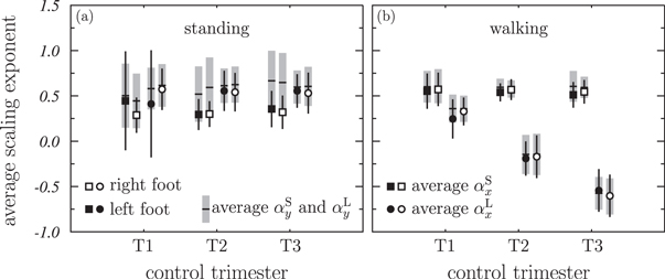
Figure 1. Average value of the scaling exponents as a function of the control trimester. Panel (a) and (b) show, respectively, the results found in standing and walking conditions. Solid (open) symbols are for the left (right) foot. Squares correspond to  and circles to
  . The corresponding standard deviations are shown with the uncertainty bars. The gray rectangles indicate the standard deviation of the scaling exponents obtained in the y direction and the small horizontal dashes show the corresponding average values.
Download figure:
Standard image High-resolution imageAlso, there is a good agreement between the values found for the x coordinate (represented by the open and solid symbols) and those corresponding to the y direction (shown by the gray rectangles). The only exception is that of the exponents (open and solid squares), in standing conditions (left panel), for the 2nd. and 3rd. trimesters: in these cases the average  values appear to be smaller than those found in the y direction, with p < 0.05, though the results agree within the statistical standard deviation. In all the other cases p > 0.05.
In standing conditions (left panel), the average small-τ end  scaling parameters (open and solid squares) coincide, within the uncertainties, with the large-τ end
  ones (open and solid circles), all of them being around 0.5. The same occurs for the corresponding y average exponents (shown with the gray rectangles). All the comparisons show p-values above 0.05 except in the case of the αS exponents for the last two trimesters mentioned above.
However, in walking conditions (right panel) a different behavior is observed. Therein we can see that the large-τ end average scaling parameters reduce significantly (p < 0.05) along the pregnancy, reaching values of the order of −0.5 in the 3rd. trimester. On the contrary, the small-τ end ones do not change, remaining at ∼0.5 as in standing conditions, with p-values well above 0.05. The negative values of the scaling parameters  indicate that the fluctuations reduce with the scale of observation, the signal becoming smoother for increasing scales.
The results obtained indicate that the foot CoP trajectories show a multi-scaling character, a feature that is accentuated as pregnancy progresses: the differences between the average scaling exponents obtained at the small-τ and the large-τ ends of the DFA scaling functions increase significantly from the 1st. to the 3rd. trimester.
It is also interesting to look at these results in terms of the quantity δ, defined in equation (9). Figure 2 shows the δ values, averaged over the whole woman sample, as a function of the control trimester. The values found in standing conditions (left panel) are practically constant and close to 0, indicating that, in average, the plantar CoP trajectories do not show multi-scaling effects. However, the average δ's obtained for walking women (right panel) grow as pregnancy progresses, pointing out a change of the scaling properties of the signals analyzed between small-τ and large-τ scales.

Figure 2. Average value of δ, defined in equation (9), as a function of the control trimester. Panels (a) and (b) show, respectively, the results found in standing and walking conditions. Solid circles and open squares stand for δx calculated for the left and right feet, respectively. The corresponding standard deviations are also shown with the uncertainty bars.The gray rectangles indicate the standard deviation of δy and the small horizontal dashes show the corresponding average values.
Download figure:
Standard image High-resolution imageWe also investigated the behavior of δ for each individual woman in our sample by calculating, for each of the three control trimesters and for both standing and walking conditions, the quantities δx and δy for both feet. In general the four values obtained showed up to be rather similar and, to summarize the information, their average and standard deviation were determined. Results are shown in figure 3 for the 42 women for whom the complete experimental information was available. The overall behavior observed in the average δ data of figure 2 can be seen here too. Except in a few cases the values found in standing conditions (open squares) stay close to 0 and show changes much smaller than those corresponding to walking women (solid circles).

Figure 3. Average values of δ, defined in equation (9), as a function of the control trimester for each women in our sample. Only the results corresponding to the 42 women having the complete set of data are shown. Open squares and solid circles correspond, respectively, to standing and walking conditions. The averages have been obtained for the four data available in each case: left and right feet and x and y signals. The corresponding standard deviations are also shown with the uncertainty bars.
Download figure:
Standard image High-resolution imageThe results obtained in standing conditions differ from those found in previous works for the CoP of the whole body, for which a multi-scaling behavior is found (Duarte and Zatsiorsky 2001, Blázquez et al 2012). In the latter case, an anti-persistent behavior of the trajectory occurs for large τ values, when the body disequilibrium reaches situations where the falling risk becomes non-negligible. The individual foot signals that we have measured here do not show such behavior in standing conditions but it appears very clearly in the walking outcomes.
The technique described here permits to study the variations in the walking characteristics of pregnants, based on a mathematical analysis of the trajectories of the center of pressure of both feet.
In previous works (Ribas and Guirro 2007, Karadag-Saygi et al 2010, Zhang et al 2015, Mei et al 2018), both anteroposterior and medio-lateral large shifts were observed in the plantar CoP trajectories measured for pregnant women, with respect to those found for non-pregnant ones. This feature became more evident as pregnancy progressed.
The fact that the  exponents obtained in our analysis are clearly smaller than 0.5 for the walking CoP trajectories, could be related to these shifts. The small, even negative, values of these exponents indicate that the walking CoP trajectories behave in an anti-persistent way in the large-τ scale. This could be at the base of the mechanisms activated by pregnant women when they try to counteract the risk of falling that increases as pregnancy progresses.
4. Conclusions
The fractal behavior of the trajectories of the foot centers of pressure in pregnant women was investigated, paying special attention to its evolution as pregnancy develops. Both standing and walking signals for 71 women were collected in the three trimesters of the pregnancy. The analysis of the trajectories was carried out by means of the DFA technique and the scaling exponents corresponding to the small and large ends of the respective scaling functions were extracted and compared.
No differences have been observed between the exponents corresponding to the x and y coordinates and to both feet. In the case of the standing data the exponents found at the two fractal scales analyzed were around 0.5 and remained practically constant through pregnancy. The situation was different for walking data where the large-end exponents reduced considerably with respect to the small-end ones, which maintained roughly the same value as in the standing case. The observed effect increased as pregnancy progressed.
This increase of the anti-persistent behavior of the plantar CoP trajectories may be linked to a displacement in the foot anteroposterior and medio-lateral pressure balances already observed in different previous experiments.
Acknowledgments
This work has been supported in part by the Junta de Andalucía (FQM0387, FQM0362, P07-FQM03163, P10-TIC5997).
: Appendix. Details of the calculations
In this appendix, details of the calculations carried out to obtain the scaling exponents are given in order to address some open questions about the procedure we have followed.
Figure 4 shows the whole information corresponding to the y signals, right foot, of subject #31, both in standing (left panels) and walking (right panels) conditions. The original, spatial-like, signals are shown in panels (a) and (b). The length of the standing signal is smaller that that of the walking one. This is a general characteristic of our data set. On the other hand, the walking signal shows the expected pattern because of the periodic loss of pressure when the foot does not rest on the ground. The velocity-like signals, obtained by subtracting consecutive values of the original ones, are shown in panels (c) and (d).
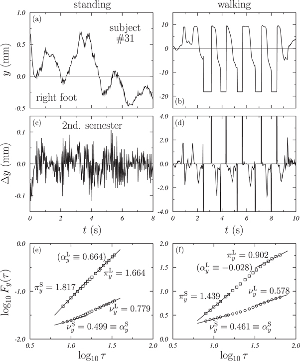
Figure 4. Results corresponding to subject #31. The data plotted are for the y signal of the right foot. Left and right panels are for standing and walking conditions, respectively. Panels (a) and (b) show the original signals. Panels (c) and (d) show the respective velocity-like signals. Panels (e) and (f) are the log-log plots from which the scaling exponents are extracted. Here the squares stand for the signals in panels (a) and (b), while the circles correspond to the velocity-like signals shown in panels (c) and (d).
Download figure:
Standard image High-resolution imagePanels (e) and (f) show the log-log plots obtained from the respective signals and used to extract the scaling exponents. In the examples shown we see how the curves behave linearly at these ends. As indicated in subsection 2.4, the linear fits providing such exponents were carried out by considering the four point closest to the small and large ends of the curves. We checked that there are no significant changes if instead three or five points are considered.
The values of the scaling exponents obtained in all cases are also given. In principle, and according to equation (8), it should be verified that νy = πy − 1. However, in the case we are analyzing, this is well satisfied only for the small-τ end of the walking signal. It is also approximately accomplished for the large-τ end of the standing one. But this condition is largely violated in the other two cases. This is the reason why, as explained in subsection 2.4, the exponents considered in this case as those adequately representing the scaling properties of the signal analyzed are  and
and  .
.
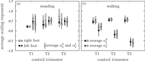
Finally, it is worth to give a look to the role played by the length of the signals. As indicated in table 2, we have analyzed signals with different lengths M. As the size τ of the subseries analyzed ranges between 8 and M/10, the values at the respective large ends would be different and this could affect the  scaling parameters. In order to check this we have repeated the analysis producing the figure 1 but neglecting all signals having less than 500 points. Figure 5 show the results obtained. As we can see the differences with figure 1 are small and the overall findings occur in a very similar way.
Figure 5. Same as in figure 1 when all the signals with less than 500 points are not included in the analysis.
Download figure:
Standard image High-resolution image