


ABSTRACT
We present the first Hubble Space Telescope Wide Field Planetary Camera-2 imaging survey of the entire Crab Nebula, in the filters F502N ([O iii] emission), F673N ([S ii]), F631N ([O i]), and F547M (continuum). We use our mosaics to characterize the pulsar wind nebula (PWN) and its three-dimensional structure, the ionizational structure in the filaments forming at its periphery, the speed of the shock driven by the PWN into surrounding ejecta (by inferring the cooling rates behind the shock), and the morphology and ionizational structure of the Rayleigh–Taylor (R-T) fingers. We quantify a number of asymmetries between the northwest (NW) and southeast (SE) quadrants of the Crab Nebula. The lack of observed filaments in the NW, and our observations of the spatial extent of [O iii] emission lead us to conclude that cooling rates are slower, and therefore the shock speeds are greater, in the NW quadrant of the nebula, compared with the SE. We conclude that R-T fingers are longer, more ionizationally stratified, and apparently more massive in the NW than in the SE, and the R-T instability appears more fully developed in the NW.
Export citation and abstract BibTeX RIS
1. INTRODUCTION
The Crab Nebula is the remnant of a Type II core-collapse supernova explosion, observed on Earth by Chinese astrologers on July 4, 1054 AD, and by Arab astronomers possibly as early as April 11, 1054 AD (Collins et al. 1999). We refer the reader to Hester (2008) for an extensive review of this supernova remnant, which comprises three separate but interdependent components. Near the center of the nebula is the pulsar, whose spin-down luminosity energizes and accelerates outward the surrounding pulsar wind nebula (PWN). The expansion of the PWN has been modeled by Jun (1998), Bucciantini et al. (2004), and others. About 2 pc from the pulsar, at the boundary of the PWN, where it encounters the ejecta from the supernova, filaments composed of the ejecta can be found. These are observed through visible line emission arising both from radiative cooling behind the shock driven into the freely expanding ejecta by the PWN (Sankrit & Hester 1997; hereafter SH97), and from photoionization of the gas by synchrotron radiation emitted by the PWN (Sankrit et al. 1998). As the low-density pulsar wind accelerates into the denser ejecta, the contact discontinuity between them is subject to Rayleigh–Taylor (R-T) instabilities (Chevalier & Gull 1975; Bandiera et al. 1983; Davidson & Fesen 1985). This instability manifests itself as finger-like protrusions pointing from the interface toward the center of the remnant. The growth of R-T instabilities in the Crab Nebula has been studied in the non-magnetic (Jun 1998) and magnetic (Bucciantini et al. 2004; Stone & Gardiner 2007) regimes. The morphology of the remnant overall, and these "R-T fingers" in particular, provide important clues to the overall structure and evolution of the Crab Nebula.
R-T instabilities like those observed in the Crab occur only when a low-density gas is accelerated into a high-density gas, but only under specific conditions. If the gas in the vicinity of the R-T fingers were not magnetic, R-T fingers would naturally arise, because the pulsar wind is of low density and high pressure and is accelerating the high-density ejecta surrounding the PWN. A magnetic field with strength B ∼ 300 μG (Trimble 1968), presumably parallel to the contact discontinuity, does exist within the PWN, which means that the discontinuity will be subject to magnetic R-T (or Kruskal-Schwarzschild) instabilities, under restrictive conditions. In such a situation, a threshold for instability exists because the inertia of the high-density gas must overcome the magnetic tension force, thus requiring a minimum gas density or acceleration (Chandrasekhar 1961). (But see Stone & Gardiner 2007, who argue that the R-T instability is not always suppressed by strong magnetic fields.) More specifically, instability requires ρejg > (B2/4πλ), where ρej is the ejecta density (assumed to be much greater than the pulsar wind density), g is the effective gravity or acceleration, and λ the radius of curvature of the field lines, essentially the wavelength of the instability. Hester et al. (1996) showed that magnetic field strength, the density and acceleration of the gas, and the wavelength of the instability together just satisfy the relationship for the magnetic R-T instability. Based on the changing expansion speed of the nebula (Trimble 1968) we estimate g ∼ 10−3 cm s−2, and observations suggest λ ∼ 3 × 1016 cm (Hester et al. 1996). The R-T instability requires both an acceleration and a minimum density ρej/mH > ρcrit/mH ≈ 140 cm−3. This critical density is comparable to the gas densities inferred by Fesen et al. (1997). We conclude that R-T finger formation can occur, but its growth is probably sensitive to the exact conditions in the Crab Nebula.
A northwest–southeast (NW–SE) asymmetry in the morphology and development of R-T fingers has been noted, suggesting some difference in environmental conditions or histories. R-T fingers in the NW are longer than R-T fingers in the SE (Loll et al. 2007; Hester 2008; Loll 2010). Jun (1998) suggested either the instability initiated sooner in the NW, or that it operated faster in the NW. Hester (2008) suggested the ejecta densities were lower, and the shock speeds and accelerations higher in the NW. Charlebois et al. (2010) disputed whether the density in the NW was lower (they inferred a lower electron density there), but they did consider the R-T instability to have developed "faster" in the NW. Beyond these suggestions, there so far has been relatively little research devoted to the asymmetrical development of the R-T instability.
Other NW–SE asymmetries have also been noted in the morphological properties of the Crab Nebula. In the NW, the PWN extends beyond the boundary of the visible line emission, whereas in the remaining 3/4 of the PWN's perimeter the pulsar wind is confined by filaments (Velusamy 1984). SH97 attributed this asymmetry to differences in the speed of the shock driven by the PWN into the freely expanding ejecta. SH97 computed atomic cooling rates in post-shock gas and determined that for shock speeds greater than ≈180 km s−1, the post-shock gas is heated to temperatures that are too high to allow the rapid cooling necessary to form filaments; for shock speeds >195 km s−1, the shocked gas does not cool over the lifetime of the Crab Nebula. They suggested that in the NW the ejecta density is lower than in the SE, such that in the NW alone the shock speed is ≫180 km s−1, too high to form filaments; in this region, the PWN can accelerate past the visible filaments. In a region observed by Blair et al. (1992), near the equatorial region of the PWN, SH97 computed (on the basis of line ratios) lower shock speeds (Vs ≈ 150 km s−1) that would lead to shorter cooling times and the formation of filaments that confine the PWN. This explanation appears valid, but leaves unanswered why the NW differs from the SE, and what the evolutionary history of the Crab Nebula has been.
In this paper, we present new observations of the Crab Nebula that we use to quantify many various NW–SE asymmetries, and we discuss how these asymmetries might have arisen. In Section 2, we present the results of the only Hubble Space Telescope Wide Field Planetary Camera-2 (HST WFPC-2) survey to cover the entire Crab Nebula. The survey includes eight WFPC-2 fields taken between 1999 October and 2002 January in the following filters: F502N ([O iii]), F673N ([S ii]), F631N ([O i]), and F547M (a filter admitting a relatively line-free continuum). In Section 3 we use these observations to quantify several NW–SE asymmetries that have been previously noted, such as the length of R-T fingers and the wavelength of the R-T instability, as well as many NW–SE asymmetries that have not been noted previously, including the ionizational structure of the filaments and R-T fingers.
2. OBSERVATIONS
We present the results of the first HST WFPC-2 dataset to cover the entire Crab Nebula at 0 1 resolution. Eight WFPC-2 fields were imaged between 1999 October and 2002 January, in the following filters: F502N ([O iii]), F673N ([S ii]), F631N ([O i]), and F547M (a filter admitting a relatively line-free continuum). The exposure times for the [O iii] images were 2600 s, the [O i] images were exposed for 1300 s, the [S ii] images were exposed for 1300 s, and the F547M images were exposed for 900 s. Table 1 provides the exposure dates and pointing information for this data set, and Figure 1 shows the locations and overlap of each WFPC-2 field. Cosmic rays were removed from the emission line images using coincidence rejection techniques with multiple observations. Due to only having a single observation of the continuum images, cosmic rays were removed from the continuum images by flagging pixels with intensities higher than 2.5σ with respect to surrounding pixels, and replacing those pixels with an average intensity of surrounding pixels. Finally, to minimize the appearance of "seams" between adjoining WF and PC chips in the mosaics presented here, linear interpolation was applied over approximately 30–60 pixels on either side of the seam (based on the signal-to-noise ratio around a seam) between the adjoining chips for a given WFPC-2 field. For purposes other than the mosaics, any data extraction near seams was carried out on the non-interpolated data, which we retained.

Figure 1. The field map for these HST observations presented in Table 1. North is up and east is to the left.
Download figure:
Standard image High-resolution imageTable 1. Exposure Dates and Pointing Information for HST Observations
| Exposure ID | Field | Filter | Date | R.A. | Decl. |
|---|---|---|---|---|---|
| (U5D10) | (UT) | (° ' '' (J2000)) | (° ' '' (J2000)) | ||
| 101R | 1 | Cont | 2000 Jan 27 | 05 34 23.24 | +22 00 06.17 |
| 102R, 103R, 104R | [O i] | ||||
| 105R, 106R | [O iii] | ||||
| 107R, 108R | [S ii] | ||||
| 201R | 2 | Cont | 2000 Jan 26 | 05 34 25.44 | +22 02 34.27 |
| 202R, 203R, 204R | [O i] | ||||
| 205R, 206R | [O iii] | ||||
| 207R, 208R | [S ii] | ||||
| 301R | 3 | Cont | 1999 Oct 24 | 05 34 28.99 | +21 59 48.08 |
| 302R, 303R, 304R | [O i] | ||||
| 305R, 306R | [O iii] | ||||
| 307R, 308R | [S ii] | ||||
| 401R | 4 | Cont | 2000 Dec 3 | 05 34 30.97 | +22 02 11.34 |
| 402R, 403R, 404R | [O i] | ||||
| 405R, 406R | [O iii] | ||||
| 407R, 408R | [S ii] | ||||
| 5501R | 5 | Cont | 2000 Jan 28 | 05 34 40.31 | +22 01 13.07 |
| 502R, 503R, 504R | [O i] | ||||
| 505R, 506R | [O iii] | ||||
| 507R, 508R | [S ii] | ||||
| 601R | 6 | Cont | 2000 Jan 29 | 05 34 38.46 | +21 58 54.65 |
| 602R, 603R, 604R | [O i] | ||||
| 605R, 606R | [O iii] | ||||
| 607R, 608R | [S ii] | ||||
| 701R | 7 | Cont | 1999 Oct 11 | 05 34 42.83 | +21 59 42.99 |
| 702R, 703R, 704R | [O i] | ||||
| 705R, 706R | [O iii] | ||||
| 707R, 708R | [S ii] | ||||
| 801R | 8 | Cont | 2002 Jan 9 | 05 34 35.15 | +22 03 50.92 |
| 802R, 803R, 804R | [O i] | ||||
| 805R, 806R | [O iii] | ||||
| 807R, 808R | [S ii] |
Download table as: ASCIITypeset image
After each WFPC-2 field was assembled for all four filters, we began creating the eight-field mosaic using the astrometry information from an image of the Crab Nebula taken with the Very Large Telescope (VLT), available in the European Southern Observatory (ESO) archives under program ID 60.A.9203(C). Astrometry information on 73 stars that were in the field of view of both the VLT and HST images, and which had accurate positions listed in the General Star Catalog II (GCS-2), were used to apply a linear and rotational transformation to the HST images using the Interactive Data Language (IDL) routine xfitgsc2. The end result was stellar astrometry in each HST field that was identical to the astrometry of those same stars in the VLT image.
The stellar astrometry and the alignment of the fields are nearly exact, but disparities in the alignment of features such as the expanding filaments may still exist because of the time differences between the various HST observations (Table 1). Trimble (1968) determined that the filaments expand approximately homologously away from the explosion center (EC), with average velocities ≈1500 km s−1 at the edge of the nebula. Assuming this expansion speed, we can estimate the misalignment of filaments that span adjacent fields. The overlapping fields that may have offsets of 0.5 pixels or greater include Fields 3 and 4, which were observed over a year apart. Features observed in their overlapping region would be separated by 1.8 pixels if they were moving at 1500 km s−1. This region of overlap, however, is situated near the center of the nebula, so that displacements in the plane of the sky are reduced by factors of a few, so that the displacements are <1 pixel =01 ∼0.001 pc. (Throughout this paper we assume a distance to the Crab Nebula of 2 kpc, so that 1'' = 0.01 pc.) Fields 4 and 5, observed 10 months apart, share a thin region of overlap. The displacements of features across this region may reach a maximum of 1.3 pixels. Offsets of 0.5 pixels may be expected between fields 7 and 5 and also between fields 7 and 6. The most shifted features are across the overlap region between fields 8 and 4 (1.7 pixels) and fields 8 and 5 (3.1 pixels), which are in the NE quadrant of the nebula. Excluding this region, all other offsets amount to about a pixel or less. For our current purposes, even a 3-pixel offset has little effect on conclusions of this paper. We seek variations in distances ≳ 1% of the nebula radius, or ≈20 pixels across.
The HST fields that cover regions outside of the nebula all had minor differences in the pixel values. To correct for Digital Charge (DC) offsets between different HST observations, we chose field 5 (Figure 1) as the standard for background scaling for each line emission image and the continuum, due to it having the largest area of sky outside of the nebula and because field 5 overlaps three other WFPC-2 fields. Beginning with that field, an adjacent field was added to the mosaic and intensity was measured over regions where the two fields overlap in an area where there was the least amount line emission. A linear scaling was determined that would make the data vary smoothly from one field to the next until eventually all eight fields were included.
The mosaics presented in this paper have been reconstructed so that there is only one resampling of the data. This was possible by mapping the x, y locations of each pixel of each WF and PC chip after both the rotational and linear transformations were applied to give the correct (VLT) astrometry. The pixel map was identical for the same chip in the same field (for example, WF1 of field 8), regardless of the filter. We then applied an algorithm that placed WFPC-2 chips that had DC corrections applied and cosmic rays reduced directly into the correct astrometric position in the mosaic. There were areas where the seams between chips were visible or there was not complete overlap, and in those regions data from the original (resampled) mosaic was used.
The HST mosaics were converted to flux values by using the standard pipeline calibration in the HST manual and then were corrected for interstellar reddening by using the standard interstellar extinction curve given in Table 7.1 of Osterbrock (1989). The accuracy of our calibration was compared to published spectra of the Crab by Fesen et al. (1997) by smoothing the HST images to the resolution of the ground-based observations and then measuring line intensities at the Fesen et al. (1997) locations. We find that the fluxes we measure in the HST image differ from the values quoted by Fesen et al. (1997) by up to 30%. Although this may seem like a fairly large discrepancy, factors to consider are the expansion of the nebula since the Fesen et al. observations, positional errors of the apertures onto the HST dataset, and varying shapes of the apertures used in the ground-based observations. The intensities of the emission lines are known to vary dramatically over small spatial scales and even small errors in our placement could lead to the differences in intensity that we measure here. We consider the flux calibration acceptable.
We note that narrowband line filters like the ones used in these observations are not ideal for observing the Crab Nebula, because the ejecta are moving at speeds of up to 1500 km s−1 (Trimble 1968) and emission at these velocities is Doppler-shifted outside the HST narrowband filters. Due to this limitation, the emission lines are best sampled near the edge of the nebula where the motions are in the plane of the sky. Near the center of the nebula, where the ejecta has the highest radial velocity, Doppler shifting is most problematic. Table 2 summarizes these limitations of each filter used in this study. [S ii], being a doublet, has the best velocity coverage of the three emission lines.
Table 2. HST Filter Bandpass Properties
| Filter | Δλ | Line ID | Velocity Range |
|---|---|---|---|
| (Å) | (km s−1) | ||
| F673N | 6709–6756 | [S ii] λ6717 | −306 to +1740 |
| [S ii] λ6731 | −980 to +1110 | ||
| F502N | 4999–5026 | [O iii] λ5007 | −480 to +1140 |
| F631N | 6291–6321 | [O i] λ6300 | −429 to +1000 |
Download table as: ASCIITypeset image
The three emission line mosaics ([O i], [S ii], [O iii], shown with continuum subtraction) and the continuum mosaic are shown in Figures 2–5, respectively. A colored combination of all four filters is shown in Figure 6, where red is the continuum, green is [S ii] + [O i], and blue is [O iii]. In all of the mosaics, north is up and east is to the left.

Figure 2. The [O i] HST mosaic. North is up and east is to the left.
Download figure:
Standard image High-resolution image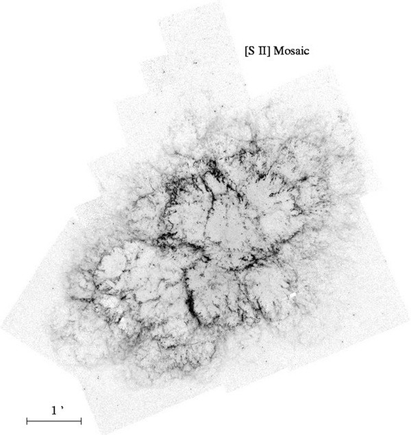
Figure 3. The [S ii] HST mosaic. North is up and east is to the left.
Download figure:
Standard image High-resolution image
Figure 4. The [O iii] HST mosaic. North is up and east is to the left.
Download figure:
Standard image High-resolution image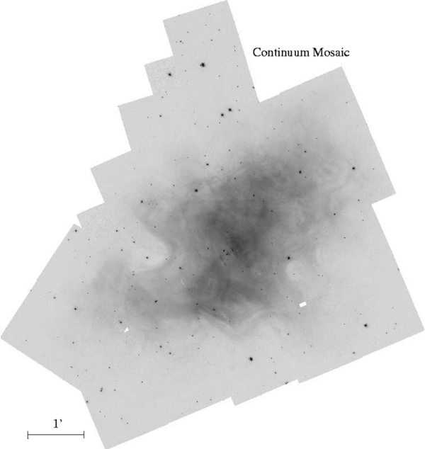
Figure 5. The Continuum HST mosaic. North is up and east is to the left.
Download figure:
Standard image High-resolution image
Figure 6. The composite of all four HST filter WFPC-2 mosaics of the Crab Nebula. [O iii] λ5007 is shown in red, [S ii] λλ6717, 6731 in green, and the [O i] λ6300 and continuum are blue. North is up and east is to the left.
Download figure:
Standard image High-resolution image3. OBSERVATIONAL RESULTS
Our observations of the Crab Nebula make apparent several NW–SE asymmetries, which we quantify here. Lawrence et al. (1995) used Fabry–Perot data to produce three-dimensional images of the Crab and concluded that the boundary between the PWN and surrounding ejecta was well fit by a prolate ellipsoid that has a tilt of about 25° into the sky. We use this information along with our measured two-dimensional distances (projected on the sky) to determine the actual length of the major and minor axes of the nebula and the symmetry axis of the nebula. We then analyze the ionization structure at the edge of the nebula in our line of sight, in individual filaments near the center of the nebula (along our line of sight), and in the R-T fingers. We demonstrate many differences between the NW and SE poles of the nebula, which are consistent with lower pre-shock ejecta densities and higher shock speeds in the NW as compared with the SE. Finally, we examine R-T finger morphology in the two regions to show that fingers appear longer, more massive, and more widely separated in the NW than in the SE.
3.1. Three-dimensional Structure of the Nebula
To provide context for the analysis that follows, establish the symmetry axis of the PWN, and determine the distances from the pulsar and EC to the edge of the nebula, we measured the boundary of the PWN on the plane of the sky and then assumed a tilt angle of 25° into the sky (Lawrence et al. 1995) to calculate the lengths of the major and minor axes. The edge of the PWN can be defined by the edge of the radio synchrotron emission, which corresponds to the contact discontinuity, or by the [O iii] emission in the filaments and cooling region behind the shock. These edges are coincident for the most part, with exceptions discussed below. To constrain the outer edge of the PWN, we utilized Very Large Array (VLA) radio data of synchrotron emission from Bietenholz & Kronberg (1990), and our own HST [O iii] images. In practice, the radio and [O iii] emissions fall off sharply beyond the edges of their strong emission, allowing a boundary to be identified. We determined the location of each boundary by eye using a surface brightness cutoff. We estimate a maximum uncertainty in the boundary location of 10 pixels (=1'', or ≈0.01 pc). The x–y coordinates of both the radio and [O iii] edges were fit to a closed elliptical curve using the Interactive Data Language program mpfitellipse developed by Craig Markwardt (NASA/GSFC). Figure 7 shows the mapped outer edges and best-fit ellipses to both the synchrotron nebula (red, χ2ν = 2.6) and the [O iii] emission (green, χ2ν = 0.92). The centers of the ellipses are represented by a red triangle for the PWN and a green square for the [O iii] emission. The current location of the pulsar (white asterisk) and the approximate EC (white cross), determined by Kaplan et al. (2008), are also indicated. The centers of both ellipses are near the pulsar but are not coincident.
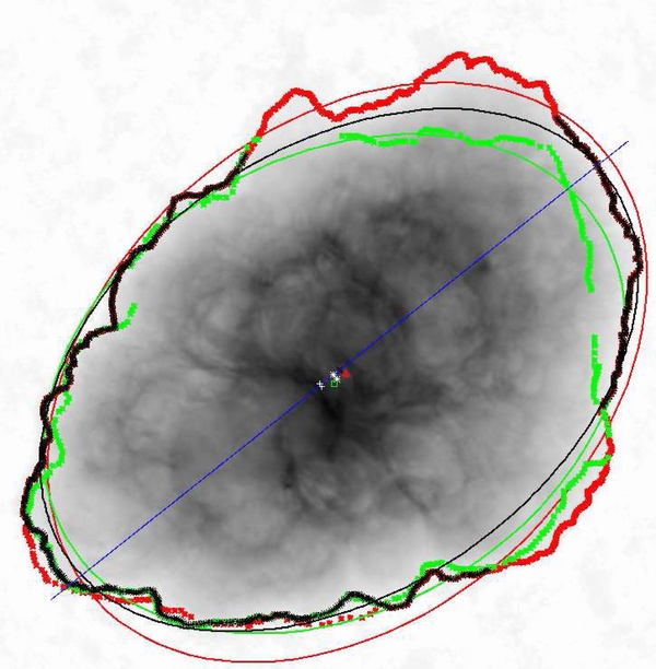
Figure 7. VLA radio image of synchrotron emission from the Crab Nebula, from Bietenholz & Kronberg (1990). Overlain on the image are the best-fit ellipses corresponding to the outer radio edge of the synchrotron nebula (red) and to the [O iii] emission (green). The black ellipse was created by using portions of both the [O iii] emission and radio data in regions where their edges are well defined and coincident. It represents the best-fit ellipse. In regions where the edge was not well defined, or where there were lobes outside of the ellipses, no data were used. The center of each ellipse is represented by a symbol of the same color. The pulsar is currently located at the white asterisk, and the expansion center is located at the white +, and the projection of both onto the major axis is also shown. The projection of the major axis onto the plane of the sky is shown in blue.
Download figure:
Standard image High-resolution imageOur goal is for the ellipse to coincide with the PWN boundary at the NW and SE poles, and the equatorial region of the nebula, as closely as possible. Fitting the ellipse to just the [O iii] emission or just the radio emission will lead to discrepancies. The [O iii] emission (green) does not reach the edge of the shock in the NW region of the nebula because the [O iii] emission is dominated by filaments that have lagged far behind the radio-emitting gas. The ellipse fit to the radio boundary does not correlate with the visible boundary in the SE part of the nebula. To create a more sensible fit to the boundary of the nebula, we generated a third ellipse using only those points where we consider the edge to be well defined. Near the NW pole and moving southward, we used the radio synchrotron mapping of the PWN, because the PWN has clearly advanced past the visible filaments. Throughout the entire south and SE end of the PWN, the [O iii] boundary is coincident (to within 14'') with the radio boundary. In those locations we use the [O iii] emission where possible to define the boundary because it usually has a higher surface brightness and more sharply defines the boundary, but near the equatorial regions the filaments are faint and the boundaries are more accurately defined using the radio emission. In other locations the boundary is difficult to define and we did not use either the radio or [O iii] data to in those locations in our ellipse fit. This includes a lobe of emission in the SW, and a region in the north where the PWN has erupted into the surrounding medium. This area has a feature that has been described as the "chimney" or a "jet." The points we do include in our ellipse fitting are colored black in Figure 7. By these criteria we produced our best estimate of the edge to the PWN and we fit the black ellipse to these boundary points. The center of that ellipse is represented as a black × in Figure 7. While the criteria used to produce this ellipse are somewhat arbitrary, the black ellipse not only is mathematically a good fit to the black boundary points (χ2ν = 0.9), it also matches the fit to the green ([O iii]) ellipse in the SE while still encompassing PWN gas in the NW, with a boundary coincident with the radio emission. The symmetry axis of this ellipse also has the same position angle, 125°, as that derived by Lawrence et al. (1995). The black ellipse in Figure 7 is our best approximation to the average shape of the PWN. The major axis, pulsar location, EC, as well as the projected locations of the pulsar and EC onto the major axis are also shown in Figure 7.
To find distances from the pulsar or EC to the location of the outer shock, we must know the physical size of the PWN. We used the values from Lawrence et al. (1995) for the tilt of the nebula into the sky, ψ ≈ 25°, and a position angle of 125°, to model the PWN as a three-dimensional prolate ellipsoid. It is natural to assume that the PWN is elongated because of the displacement of the pulsar, in which case a naturally arising symmetry axis of the nebula would be one that connects the EC (Kaplan et al. 2008) and the coordinates of the pulsar in the HST image. Our derived symmetry axis is very nearly aligned along this direction, to within a few degrees. The pulsar lies only 1'' (0.01 pc) from this axis, and the EC about 7'' (0.07 pc) from this axis. For ease of calculation when determining distances from the EC or pulsar to points on the PWN boundary, we shift the assumed positions of the pulsar and EC by these amounts along the NE–SW direction, so that their assumed positions lie on this axis (shown in Figure 7). We find the pulsar lies 50 (0.048 pc) SE of the center of the ellipsoid, and 13'' (0.13 pc) NW of the EC.
It is straightforward to show that if an ellipsoid with semi-major and semi-minor axes a' and b' = b is tilted about its minor axis into the sky by an angle ψ, its projection will be an ellipse with semi-major and semi-minor axes a and b, with
The minor axis of the ellipsoid necessarily matches the minor axis of its projection (our black ellipse in Figure 7). Our best-fit ellipse above has semi-minor axis 1.43 pc and projected (apparent) semi-major axis 2.13 pc. Using ψ = 25°, we compute a semi-major axis of 2.25 pc for the three-dimensional ellipsoid.
Use of different emission maps (e.g., [O iii] versus radio) can introduce variations in the fit to this boundary of several percent. Even so, one obvious feature from Figure 7 is that the edge of the PWN is approximately, but not exactly, centered on the pulsar (white asterisk). Using the locations of the pulsar and EC when projected onto the major axis of the ellipsoid, we conclude that the NW pole is 17% farther from the EC (white +) than the SE pole, but only 4% farther from the pulsar (± < 1% due to shifting the positions of the pulsar and EC). In other words, during the expansion history of the nebula, the PWN has remained close to centered on the location of the pulsar despite the pulsar's NW proper motion.
3.2. Ionization Structure
The HST emission line mosaics include the entire nebula in low-, intermediate-, and high-ionization emission lines; they therefore are an ideal way to study the spatial ionization structure of the gas, filaments and R-T fingers. SH97 have hypothesized that the NW is characterized by faster shock speeds, >195 km s−1, which raise the gas to sufficient temperatures that it is prevented from cooling within the lifetime of the nebula. We can test this hypothesis by measuring the thickness of the cooling layer behind the shock, which is characterized by strong [O iii] emission. The cause of the higher shock speeds is hypothesized to be lower densities in the NW than in the SE. Our observations can be used to probe densities in filaments and R-T fingers by quantifying the degree of ionizational stratification. Because these objects are ionized primarily by radiation from the PWN, denser filaments and fingers (of a given size) could more effectively shield their interiors from this ionizing radiation, allowing [O iii] to recombine to [O i]. Spatial variations in [O iii], [S ii], and [O i] emission can reveal much about the densities within filaments and fingers. Here we use our HST mosaics to probe the likely shock speeds and densities in the periphery of the PWN, and in the filaments and fingers, and to assess the differences in these quantities between the NW and SE quadrants of the Crab.
We first consider the shocked gas at the periphery of the PWN. We took spatial profiles of [O iii], [S ii], and [O i] emission in 24 regions around the perimeter of the PWN. Each region was sampled over a spatial profile approximately 600 pixels (0.6 pc) in length and approximately 200 pixels (0.2 pc) in width. The regions are oriented radially away from the center of the nebula, and spaced in equal 15° increments in position angle (defined with respect to the center of our best-fit ellipse). The locations are shown in Figure 8, where we have also indicated the major axis as a dashed line. Starting at the SE pole, (the direction with a position angle of 125°) and proceeding clockwise, these spatial profiles are presented in Figures 9 and 10, with zero degrees representing the SE pole. Each profile straddles the PWN boundary; zero distance in each profile represents the location of the profile on the outside of the nebula, and larger distances refer to locations progressively inward. The measured intensities are integrated totals averaged over the spatial width of about 0.2 pc using the flux-calibrated and dereddened HST images. Sharp spikes in the intensity, as in the profile at 300 degrees, are due to stars falling in the profile region. None of the profiles were taken over regions where we had used interpolation over WFPC-2 seams.

Figure 8. Locations where spatial profiles (≈200 × 600 pixels) were taken. The dashed line represents the major axis of the nebula.
Download figure:
Standard image High-resolution image
Figure 9. Spatial profiles (widths ≈200 pixels) taken at 15° intervals, where zero is the SE pole and the direction is clockwise, covering the northern hemisphere of the nebula. Positive distances are measured closer to the center of the nebula. Spikes are due to stars in the profile region. 10 pixels ≈ 0.01 pc.
Download figure:
Standard image High-resolution image
Figure 10. Same as Figure 9, but beginning near the NW pole and moving clockwise to the SE pole.
Download figure:
Standard image High-resolution imageThe spatial profiles of the three emission lines can provide valuable insight into the formation of filaments behind the shock front. The [O i] line in particular, because it requires shielding from photoionization to form, should be diagnostic of density. This line is expected to be weak or absent in regions where dense filaments have not formed. Regions that show [O i] emission closer to the shock front may be inferred to have a faster rate of filament formation. Also, the intensity of [O iii] emission reflects the mass flux of ejecta passing through the shock and also how effective radiative cooling is in the post-shock gas.
We find that the profiles surrounding the equatorial belt of the nebula show the sharpest rises in [O iii] emission at the edge of the nebula, and also the highest [O iii] line intensities. Out of all the profiles in the northern half of the nebula boundary, the spatial profile taken at 90° in particular has the steepest rise in [O iii] emission (1.5 × 10⁻¹⁶ erg cm−2 s−1) over the smallest distance (150 pixels ≈0.15 pc) from the edge of the visible nebula (taken as the first measurable flux of [O iii] emission). The [S ii] and [O i] profiles also show smaller but similar peaks at this distance. On the southern half of the nebula boundary, the spatial profile at 270° shows [O iii] emission that is weaker than that measured at 90°, and almost no intermediate- or low-ionization emission until much farther (about 400 pixels ≈0.4 pc) from the edge. Instead, the steepest rise in [O iii] emission occurs in the profile at 300°, occurring within about 0.1 pc from the onset of [O iii] emission. The low and intermediate ionization lines, however, occur closer to the edge of the nebula at 315° than at 300°.
In contrast, line emission profiles near the SE (0°) and NW (180°) poles of the nebula show much more gradual rises in [O iii] emission and much lower [O iii] intensities. Sharp increases in [O iii] with increasing distance from the PWN edge, like those seen in the equatorial regions, are not seen near the poles; there are, however, marked increases in [S ii] and [O i] emission farther in from the edge that are coincident with peaks in the [O iii] intensity. At the SE pole, the peak [O iii] emission line intensities are only ∼1/3 those measured around the majority of the perimeter. The spatial profile at 105° shows a similarly weak intensity; this may be related to the presence of the "chimney" feature at this location, which is visible as two faint jets seen in [O iii] emission pointing due north. The spatial profile at 150° and 240° also show very weak line emission.
Further insights can be drawn using the [O i]/[O iii] line ratios, to measure how effectively the shocked gas has been able to cool (and recombine). For example, the [O i]/[O iii] ratios in the spatial profiles taken at 45° and 90° exceed the similar ratios taken at 225° or at 285°. This would seem to indicate that the shocked gas has been able to cool more effectively in the vicinity of the NE profiles than in other areas away from the poles. Another area that has spatial profiles that indicate shorter cooling times is the area between 315° and 345°. These areas also show higher overall [O iii] intensities, which we interpret to mean a higher mass flux into the shock region. Higher mass flux can be attributed to higher pre-shock ejecta densities and lower shock speeds there. Comparing profiles in the polar regions shows that the [O i]/[O iii] ratios are considerably higher near the SE pole, (0° and 15°) than what we measure at 180 degrees and 195°, near the NW pole. Compared with the NW quadrant, shocked gas in the SE quadrant appears to have been able to cool and/or compress more effectively, but not as effectively as some areas away from the poles.
We further demonstrate the variations in line intensity as a function of position angle in Figure 11, which shows the average intensity in each of the spatial profiles in Figures 9 and 10. These data were spatially averaged within each region, and then were heavily smoothed (using the SMOOTH function in IDL with a width of six bins). This procedure masks extreme variations, such as the fact that peak [O iii] emission in the SE pole is roughly 1/3 the value in the equatorial belt; the procedure instead emphasizes smooth variations with angle θ. The variances are σ2 = 2.7, 0.7, and 0.1, corresponding to percentage errors of 0.52, 0.95, and 0.46 for [O iii], [S ii], and [O i], respectively. The intensity of [O iii] emission appears to correlate with position angle, with maxima near the equator (around 60°–90°, and around 250°–290°), and minima near the poles (0° and 360°, with an additional minimum around 150°). Such variation would be consistent with high mass fluxes into the shock, and therefore higher ejecta densities, in the equatorial regions than at the poles. Unfortunately, because of the large uncertainties this correlation is not statistically significant. Variations in [S ii] and [O i] emission correlate more strongly with position angle. A maximum in the [S ii] emission is marginally detected near the SE pole (0 degrees), and possibly near the NE pole (180 degrees) as well. The [O i] emission appears uniform, except for a slight rise between about 250–340 degrees, between the SE pole and the southern equatorial region. This increase in [O i] emission may be due to filaments forming more rapidly behind the shock front in that region.
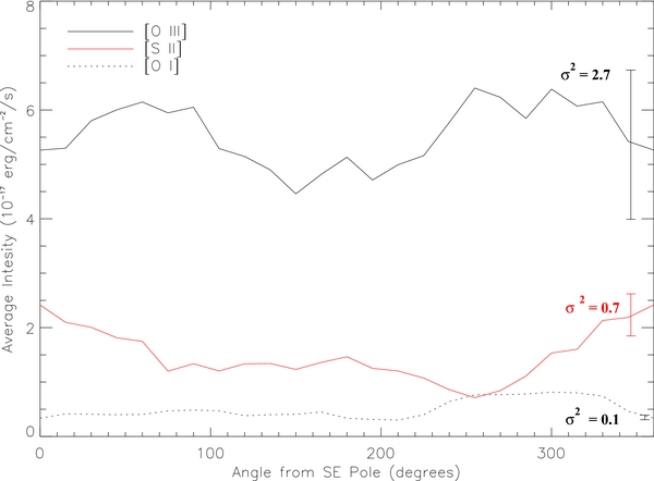
Figure 11. The average intensity of each emission line as a function of angle clockwise around the perimeter, where the SE pole is at zero degrees. The data were smoothed using the IDL SMOOTH procedure with a width of 6 bins. Error bars represent an average error for each emission line.
Download figure:
Standard image High-resolution imageWe now consider the physical properties of certain individual filaments. It has previously been pointed out that filaments are not coincident with the PWN boundary near the NW pole, and the PWN appears to have "escaped confinement" by the filaments there (SH97). This observation has been interpreted as meaning shock speeds in the NW quadrant are too high for the shock gas to cool and form filaments (SH97). Moving inward from the NW pole toward the pulsar, large-scale filamentary structures are clearly evident. These filaments lie either in front of or behind the PWN along our line of sight, and they are associated with the longest R-T fingers in the NW. These are among the filaments whose ionizational structure we wish to determine.
We determined the thicknesses of specific filaments in the NW and SE, shown in Figure 12, by measuring the width of the region of strong [O iii] emission. The spatial profiles were taken such that x = 0 represents the location in the PWN and x increases toward the shock. The plotted intensities were averaged over a spatial width of about 0.2 pc, and none of the profiles were taken at WFPC-2 seams. We find that the two filaments in the NW average 0.016 pc in thickness, 60% thicker than the 0.0097 pc average thickness of the two SE filaments. We interpret the greater thickness of [O iii] emission as indicating a longer cooling time in the NW.
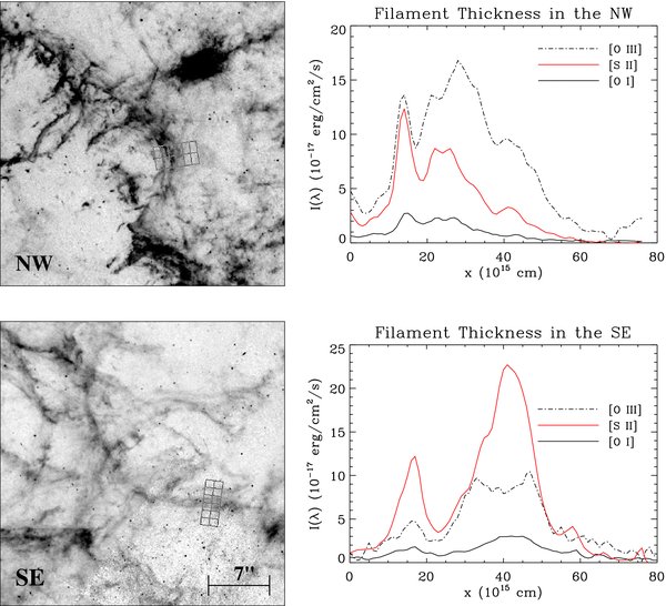
Figure 12. An [O iii] image of the NW and SE regions of the Crab including the locations where we measured emission spatial profiles (averaged over ≈0.2 pc), shown to the right of the respective image. The spatial profiles indicate the thickness of the filaments and show their ionization structures, allowing a comparison between the NW and SE quadrants of the Crab.
Download figure:
Standard image High-resolution imageThe interpretation of longer cooling times in the NW is corroborated by the ionization structures of the filaments, which show that in the NW the strengths of the various emission lines vary over the resolved scales in the images. Moving from x = 0 inward, the [O i] emission drops first, then [S ii], and finally the [O iii] emission drops. In the SE, in contrast, the drop-offs in [S ii] and [O i] emission line profiles are very nearly spatially coincident with the edges of the [O iii] emission. Another way of demonstrating this same effect is by plotting an image of the difference in intensities in [O iii] and [S ii], as in Figure 13. Figure 13(a) shows that in the SE, the [S ii] emission arises from throughout the region, and is distributed similarly to the [O iii] emission, whereas in the NW (Figure 13(b)), the [O iii] and [S ii] emissions are clearly not spatially coincident. All of these factors are consistent with shocked gas in the NW taking longer to cool than in the SE.

Figure 13. [O iii] − [S ii] images of the SE (a) and the NW (b), showing the difference in intensity in these filaments (white is positive, black is negative). In the NW, [O iii] and [S ii] emission are not as spatially coincident as in the SE.
Download figure:
Standard image High-resolution imageThe cooling time of the shocked gas around the perimeter of the nebula also may be inferred by observing the relationship between the edge of the PWN at radio wavelengths, which most closely traces the synchrotron-emitting PWN gas, and the edge of the [O iii] emission, which traces the filaments of shocked gas. In regions where the gas cools very slowly, filament growth is suppressed and the radio-emitting gas will advance beyond where the [O iii] emission arises. The PWN would then appear to "break through" the filaments. Figure 7 demonstrates that the PWN has broken through the filaments throughout much of the NW quadrant, and is beginning to do so in portions of the SE. In Figures 14–16, we compare VLA radio data (Bietenholz & Kronberg 1990) with our [O iii] images, in the southern edge of the PWN (near the equator) and the NW and SE quadrants.

Figure 14. A comparison of the [O iii] emission tracing the filaments (left), and the southern edge of the PWN as measured by radio emission (right), from Bietenholz & Kronberg (1990). Each tick mark represents 15''(or about 0.15 pc.).
Download figure:
Standard image High-resolution imageIn the south, near the equator, the radio emission is coincident with the [O iii] boundary because gas cools quickly there (Figure 14). This is also an area where the [O iii] line emission rises sharply at the edge, indicating efficient cooling (Figure 10). Figure 15 shows how the PWN has escaped the confinement of filaments in the NW due to the long cooling time of the gas, and the radio emission extends up to 0.3 pc farther out from the center of the nebula than the gas. In the SE, shown in Figure 16, we note that the PWN appears to be at or near the shock velocity that transitions from the radiative cooling regime into one that no longer forms filaments. The boundary of the PWN is more coincident with the [O iii] emission but in portions extends up to 0.08 pc beyond the boundary of the [O iii] emission. These observations provide further support that the shock speeds are higher in the NW than they are in the SE.
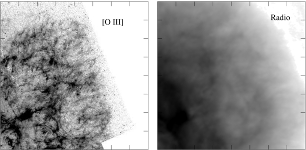
Figure 15. Same as Figure 14, but in the NW quadrant.
Download figure:
Standard image High-resolution image
Figure 16. Same as Figure 14, but in the SE quadrant.
Download figure:
Standard image High-resolution imageFinally, we consider the ionizational stratification in the R-T fingers. Mass is funneled into the tips of the R-T fingers, where the densities can reach values ten times higher than in the filaments that feed them, according to the models of Jun (1998), which follow the R-T instability into the nonlinear regime. It would not be surprising for the cores of these finger tips to be well shielded from synchrotron radiation, yielding an ionizationally stratified emission spatial profile. In fact, Sankrit et al. (1998) showed that such was the case for an R-T finger in the NW (Finger 3 in Figure 19); the exterior of the finger was seen to be bright in [O iii] emission, the core was dominantly low-ionization emission ([O i]), and [S ii] emission came from the region in between. Here we have used our mosaics of the entire nebula to conduct a similar analysis of other R-T fingers in the NW and SE regions of the Crab.
Figure 17 shows high-resolution images of two representative R-T fingers from the SE, Fingers 27 and 32 from Figure 19. The emission spatial profiles are presented to the right of each image. These show the line intensities of [O iii], [S ii], and [O i] across the tips of the R-T fingers in the corresponding images. The profiles represent average intensities along the width of the boxed regions in the corresponding image. The x-axes measure the location, with zero starting at the top center of the box in the image. The profile across Finger 27 shows [O iii] emission surrounding the finger, but the [O iii] has no clear edges denoting the boundary of the finger. The [S ii] emission is highly localized in the finger, showing a sharp edge on either side and two peaks spatially coincident with the two [O iii] peaks. The [O i] emission rises only slightly across the finger, but clearly is more spatially concentrated in the core of the finger. The line intensities of [O iii] and [S ii] across Finger 32 are only about half the values in Finger 27, but the [O i] intensity is greater. The [O iii] intensity of Finger 32 has a defined edge at the location of the finger, and the [S ii] and [O i] emission are localized in the finger, within 1 × 1015 cm of the [O iii] boundary. The higher intensity of [S ii] and [O i] within the finger, as well as their steeper spatial variation, with [O i] emission rising interior to the rise in [O iii] emission, indicates that Finger 32 is more ionizationally stratified than Finger 27.
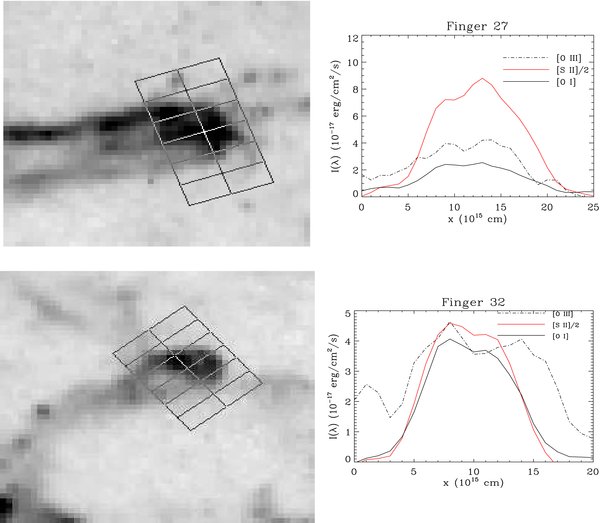
Figure 17. Locations and corresponding line intensities of R-T fingers in the SE. The pulsar is to the upper right.
Download figure:
Standard image High-resolution imageFigure 18 shows high-resolution images of two representative R-T fingers from the NW, Fingers 5 and 4 from Figure 19. The line intensity of [O iii] rises steeply at the edges of Finger 5, with two well-defined peaks, bracketing a distinct minimum in the [O iii] emission at the center of the finger. The rise in [O iii] emission is separated from the [S ii] and [O i] emission by approximately 1.5 × 1015 cm, slightly greater than the separation in Finger 27. The low-ionization lines ([S ii] and [O i]) have very similar emission line profiles, rising steeply at the edges and having two peaks. Finger 5, one of the longest R-T fingers in the Crab, is the only R-T finger we found in which the intensity of all three emission lines decreased in the core. The spatial profile for Finger 4 indicates it is another ionizationally stratified finger: It has a well-defined edge in the [O iii] emission, with [S ii] emission found about 2 × 1015 cm inward of the [O iii] edge, and [O i] even more constrained to the core than [S ii]. The [O iii] emission shows two peaks that are representative of the two edges of the R-T finger along our line of sight. The [S ii] and [O i] emission profiles, though, show only one peak each, at the very center of the finger, where we would expect the highest densities and the greatest shielding.
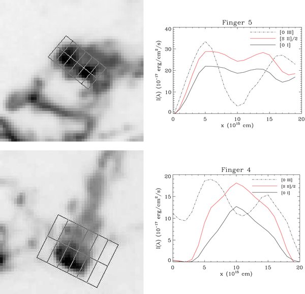
Figure 18. Locations and corresponding line intensities of R-T fingers in the NW. The pulsar is to the lower left.
Download figure:
Standard image High-resolution image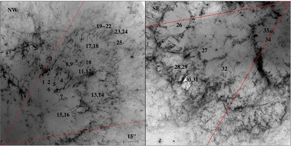
Figure 19. [S ii] images of R-T fingers in the NW and the SE quadrants of the Crab Nebula. Numbered fingers represent those included in the histogram shown in Figure 20. All selected fingers were constrained to lie within a two 25° cone aligned with the nebula's symmetry axis and with the pulsar at the apex, marked by the red diagonal lines.
Download figure:
Standard image High-resolution imageComparing these profiles, we find that the R-T fingers in the NW tend to have a more stratified ionization structure than the R-T fingers in the SE. We infer that their interiors are better shielded from ionizing radiation, and are probably denser. The tips of R-T fingers also show stronger line emission in the NW. The [O iii] and [O i] emission peaks are more than five times stronger in the NW than in the SE, while the [S ii] emission is two to three times stronger. Fabry-Perot data by Lawrence et al. (1995) indicate that the NW fingers whose profiles are shown here are seen nearly edge-on (near zero radial velocity). The fingers in the SE are too small to be resolved in the Fabry-Perot data set and therefore their radial velocity is not well known; however, fingers 27 and 32 are the two of the longest SE fingers (see below), so we would expect them to be more edge-on than the others in the SE quadrant. Thus we do not attribute these differences in line intensities to Doppler-shifting of the emission lines. The higher emission overall, combined with the greater ionizational stratification, together suggest that the tips of fingers are more massive in the NW than in the SE.
3.3. Rayleigh–Taylor Finger Morphology
One of the most obvious asymmetries seen in the HST mosaics of the Crab is the difference in length of R-T fingers between the NW and SE quadrants of the Crab. There are long, well-developed fingers throughout the NW quadrant of the Crab, but virtually nowhere else in the nebula. Here we quantify that difference by measuring the projected lengths of fingers in the both the NW and SE quadrants.
In Figure 19, we show a high-resolution image of R-T fingers in both the NW and SE regions of the nebula. The regions chosen lie along and at opposite ends of the Crab's symmetry axis, as defined in Section 3.1. Clearly, the fingers in the NW appear much longer and are more easily defined or organized than the fingers in the SE. In order to conduct a quantitative analysis of the difference in lengths, we measured the projected lengths of fingers in both the NW and SE. To minimize projection effects, we limited our analysis to those fingers within two 25° cones, centered on the pulsar and oriented along either end of the nebula's symmetry axis, as indicated by red diagonal lines in Figure 19. In order to measure a finger, we required that the tip of the finger and the base of the finger be well defined in the image, the length had to be more than a few pixels so that a measurement could be made, and the finger had to lie within the constrained area of symmetry. The fingers that met these criterion are numbered in Figure 19 and the results of those measurements are presented as a histogram in Figure 20.
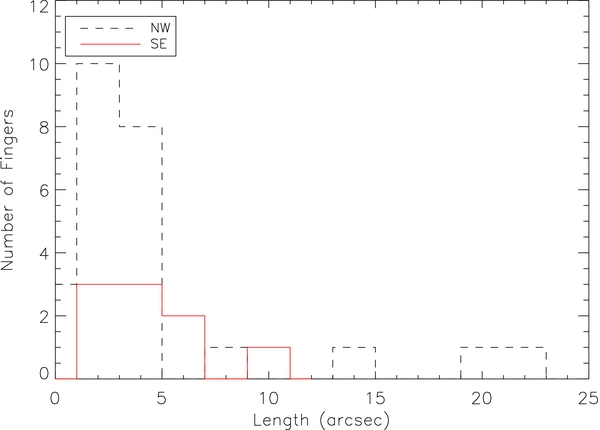
Figure 20. Histogram of the measured lengths of R-T fingers in the SE and NW regions of the nebula, within the same cones as defined in Figure 19. Bins have width 2''.
Download figure:
Standard image High-resolution imageWe find that both the NW and SE regions contain small fingers, such as fingers 11, 12, 19, 28 and 29 in Figure 19). The NW contains fingers up to 22'', whereas the longest finger in the SE is only 10''. Overall, there were 25 easily identifiable and well-developed fingers in the NW, compared with nine in the SE (at least within the constrained area). It is unlikely that these large differences in lengths or the large disparity in the number of large fingers can be attributed to projection effects, and we consider there to be a real NW–SE asymmetry in the lengths and number of R-T fingers.
Besides the lengths, the overall structure of the R-T fingers is also asymmetric. The filaments in the NW are organized—the R-T fingers and overlying filaments are isolated and easy to define—while the SE appears less developed, with about a hundred very small fingers (small enough that the lengths of such fingers could not be measured and instead appear more like perturbations at the contact-discontinuity) We attempt to quantify the level of activity of the R-T instability by determining the critical wavelength of the instability. In order to initiate the R-T instability, the separation between fingers along the contact discontinuity must exceed a critical wavelength, λcrit = B2/(4πρejg), where B is the magnetic field of the filaments, ρej is the density of the filaments, and g is the effective gravity or acceleration at the contact discontinuity (Hester et al. 1996 and references therein). If fingers are more closely spaced than this, the buoyancy of the fluid cannot overcome the magnetic tension force. On the other hand, larger separations or wavelengths grow more slowly, and the fastest growing wavelength is equal to twice the critical wavelength (Hester et al. 1996); over time, the unstable interface should evolve to a state with long fingers separated by this wavelength. Considering R-T fingers in the same restricted area where we measured R-T finger lengths, and also including filaments that showed a wavelike perturbation or cusps that have not developed into long R-T fingers but appear to be in the process of doing so (including more filaments than what was possible in the measurement of finger lengths), we were able to determine an approximate wavelength for the instability at various locations. The criterion for our measurements was that the separation of either fingers or the wave-like boundary of the contact-discontinuity was well defined along a filament and included at least two points. A histogram of our results is presented in Figure 21, comparing the NW to the SE. Our measurements indicate that the R-T instability is dominated by wavelengths of ∼1'' in the SE (average wavelength =12). In the NW, there is a tendency for the instability to take effect at a slightly larger wavelength, ∼1''–15 (average wavelength =16), and the maximum separation between fingers is to up to 35. The combination of the length and wavelength histograms reflect that although the NW appears to contain more well-developed fingers, there are actually more fingers in the SE, mostly of very short separations. The R-T instability appears to be more active right now in the SE, producing more regions that show a wave-like disturbance at the contact discontinuity; however, long fingers have not developed at those locations at this time.

Figure 21. Histogram of the measured separations of R-T fingers in the SE and NW regions of the nebula, within the same cones as defined in Figure 19. Bins have width 05.
Download figure:
Standard image High-resolution image
4. SUMMARY
We have presented the results of the first HST WFPC-2 observations to cover the entire Crab Nebula, in the four filters F502N (which tracks [O iii]), F673N ([S ii]), F631N ([O i]), and F547M (continuum). Using our mosaicked images (especially of [O iii] emission) as well as the VLA radio data of Bietenholz & Kronberg (1990), we have fit the boundary of the PWN with a prolate ellipsoid. Assuming a tilt into the sky of 25° (from the Fabry-Perot observations of Lawrence et al. 1995), we have modeled the three- dimensional shape of the PWN. We find the symmetry axis of the ellipsoid to lie 55° west of north. The EC (as defined by Kaplan et al. 2008) and the pulsar very nearly lie on this symmetry axis, and the pulsar's proper motion is consistent with motion along this symmetry axis.
We have used our modeled ellipsoid to identify asymmetries in the PWN's development. Points on the NW pole of the ellipsoid lie 17% farther from the EC than do points on the SE pole. On the other hand, points on the NW pole lie 4% farther from the pulsar than do points on the SE pole, due to the displacement of the pulsar 13'' (about 0.13 pc) to the NW. This strongly suggests that the PWN has mostly expanded away from the pulsar and not the EC, and that the pulsar has been the main driver of the PWN's outward expansion. Despite this, the PWN boundary is not centered on the pulsar, and it has developed asymmetrically even in the pulsar's frame.
Not just the current shape of the PWN is asymmetric, but so is the rate at which the PWN appears to be expanding. The PWN expands as particle and magnetic pressures drive a shock into the surrounding ejecta. Sankrit & Hester (1997) showed that the timescale for that shocked gas to cool increases monotonically with shock speed: The cooling time rises significantly for shock speeds >180 km s−1, and gas heated by a 195 km s−1 shock will not cool in the lifetime of the Crab Nebula. Our measurements of line emission intensities as a function of angle around the nebula appear to indicate that the shocked gas cools most rapidly in the areas that are away from the poles (maxima in [O iii] emission), but also that the SE pole is cooling more rapidly than the NW pole. We find the thicknesses of specific filaments (as measured by the spatial extent of their [O iii] emission) to be 60% greater than those in the SE, indicating a longer cooling time before O iii could recombine to O i. This is corroborated by the higher [O i]/[O iii] ratios in gas in the SE quadrant than in the NW. In the SE quadrant, lower-ionization [S ii] emission is spatially associated with [O iii] emission and shocked gas, and the shocked gas exhibits [S ii] and [O i] emission throughout. In contrast, [O iii]−[S ii] difference images show little spatial coincidence between the shocked gas and the [S ii] emission (which is associated instead with the R-T finger tips). This also suggests the SE has cooled more than the NW. These findings strongly suggest that the shock speeds (and therefore the PWN expansion velocity) are greater in the NW than in the SE, and apparently smallest in the equatorial region.
Around most of the periphery of the PWN, including the SE and equatorial regions, dense filaments are forming and appear to constrain the expansion of the PWN. Near the equatorial region, the PWN radio emission is spatially coincident with the [O iii] emission from the shock front. In the SE, the PWN extends in some portions up to 0.08 pc beyond the filaments. In most of the NW quadrant, in contrast, the PWN radio emission projects about 0.3 pc beyond the [O iii] emission, giving the impression the PWN has "broken through" the filaments. Filaments form as a result of R-T instabilities, and their growth rates increase monotonically with increasing density of shocked gas at the contact discontinuity. If the contact discontinuity is expanding at an accelerated rate g, has shocked gas on one side with density ρCD, and magnetic field B parallel to the discontinuity on the other, then the maximum growth rate of the R-T instability is easily shown to be σmax = (πρCD/2PPWN)1/2g (Chandrasekhar 1961), where it is assumed that the magnetic field is in energy equipartition with the particles (B2/8π = PPWN/2). It appears that post-shock gas densities are lower in the NW than in the SE. Based on the greater overall [O iii] flux, we infer that densities are highest in the equatorial regions. Post-shock densities may be increased above ejecta densities if cooling is effective, but the simplest interpretation is that the density of ejecta material decreases with distance from the EC, as expected for supernova explosions.
Our images reveal differences in the R-T fingers in the NW and SE. Our mosaics show that R-T fingers are generally longer in the NW than in the SE (maximum length 22'' compared with 10''), and that fingers in the NW are slightly more separated (15) than in the SE (10). Our maps of [O iii], [S ii], and [O i] emission reveal that R-T fingers in the NW are more ionizationally stratified and better shielded from photoionizing radiation, implying higher column densities and masses in the fingers. Likewise, the [O iii] and [O i] emission peaks are more than 5 times stronger, and the [S ii] emission 2–3 times stronger in the NW fingers than in the SE fingers, also implying higher masses. We conclude that fingers in the NW are more fully developed than those in the SE, with more mass having been funneled into them over the lifetime of the Crab Nebula. This is consistent with faster growth rates of the R-T instability in the NW than in the SE.
The observations we have presented here demonstrate that the Crab Nebula PWN is more centered on the pulsar (displaced to the NW by 13'' from the EC) than the explosion center, but that even in the frame of the pulsar, the PWN in the Crab Nebula has developed asymmetrically. The simplest interpretation is that the PWN boundary has advanced at a shock speed Vs that is comparable to (PPWN/ρej)1/2, where ρej is the ejecta density, and that ρej decreases with distance with the EC. This would yield higher shock speeds and slower R-T instabilities and filament growth rates in the NW than in the SE. Quantification of these ideas will be explored in a future paper.
We thank Jeff Hester for conceiving of this research and carrying out and making available the observations central to this work, and for useful discussions. We thank Michael Bietenholz for making available the VLA radio data used here. We thank Ravi Sankrit, William P. Blair, and Frank Timmes for their input and for personal discussions about this research. This work was supported by STScI grant HST-GO-08222.01-A and the Arizona NASA Space Grant.