


ABSTRACT
We report on the first multi-wavelength coronal observations, taken simultaneously in white light, Hα 656.3 nm, Fe ix 435.9 nm, Fe x 637.4 nm, Fe xi 789.2 nm, Fe xiii 1074.7 nm, Fe xiv 530.3 nm, and Ni xv 670.2 nm, during the total solar eclipse of 2010 July 11 from the atoll of Tatakoto in French Polynesia. The data enabled temperature differentiations as low as 0.2 × 10⁶ K. The first-ever images of the corona in Fe ix and Ni xv showed that there was very little plasma below 5 × 10⁵ K and above 2.5 × 10⁶ K. The suite of multi-wavelength observations also showed that open field lines have an electron temperature near 1× 10⁶ K, while the hottest, 2× 10⁶ K, plasma resides in intricate loops forming the bulges of streamers, also known as cavities, as discovered in our previous eclipse observations. The eclipse images also revealed unusual coronal structures, in the form of ripples and streaks, produced by the passage of coronal mass ejections and eruptive prominences prior to totality, which could be identified with distinct temperatures for the first time. These trails were most prominent at 106 K. Simultaneous Fe x 17.4 nm observations from Proba2/SWAP provided the first opportunity to compare Fe x emission at 637.4 nm with its extreme-ultraviolet (EUV) counterpart. This comparison demonstrated the unique diagnostic capabilities of the coronal forbidden lines for exploring the evolution of the coronal magnetic field and the thermodynamics of the coronal plasma, in comparison with their EUV counterparts in the distance range of 1–3 R☉. These diagnostics are currently missing from present space-borne and ground-based observatories.
Export citation and abstract BibTeX RIS
1. INTRODUCTION
The inner corona, starting from the solar surface out to heliocentric distances of 5–10 solar radii (R☉), is believed, at present, to be the region where the imprint of the physical processes responsible for heating the coronal plasma and accelerating the solar wind is the most pronounced. (In this paper, all distances are given in R☉ measured from Sun center.) It is the critical region where the solar magnetic field undergoes the most dramatic changes as it evolves from the photosphere outward into interplanetary space. The inner corona thus establishes the connection between the Sun and its heliosphere.
Prior to the space age, total solar eclipses provided the sole opportunity for exploring the plasma properties of the inner corona through imaging and spectroscopy, as the sky brightness is significantly reduced to levels below the intensity of most emission lines out to 2–3 R☉. The invention of the coronagraph by B. Lyot in 1930 (Lyot 1932) significantly expanded these opportunities by enabling daily observations in unpolarized and polarized white light and in some of the coronal forbidden lines such as Fe x 637.4 nm, Fe xiii 1074.7 nm, and Fe xiv 530.3 nm (e.g., Newkirk et al. 1970). However, imaging and spectroscopy with a coronagraph remained limited to distances above 1.05 R☉ due to diffraction at the edge of the occulter, and below 1.5 R☉ due to the limited reduction of sky brightness down to the levels experienced during totality beyond that distance.
With the advent of space exploration, the diagnostic capabilities provided by the ultraviolet, extreme-ultraviolet (EUV), and X-ray wavelength ranges gained significant momentum (e.g., Goldberg et al. 1968; Vaiana et al. 1968; Noyes et al. 1970; Gabriel et al. 1971; Beckers & Chipman 1974; Delaboudinière et al. 1995). As the opportunity to simultaneously image the corona on the solar disk and off the limb materialized for the first time, the potential to establish the sources of the intricate structures of the corona, observed during eclipses, became tenable. However, the diagnostic capabilities of the EUV lines and X-rays were also limited to distances below 1.5 R☉ due to the inherent dominance of their collisional component in the intensity of their emission, which decreases with distance as the square of the density.
Spectral lines in the ultraviolet typically above 100 nm, on the other hand, were potentially more attractive candidates because of the existence of a radiative component, which enabled the inference of the outflow velocity in the inner corona for the first time (Noci et al. 1987). However, the use of a coronagraph was essential for extending the distance range of the detectability of these lines. This approach was first successfully demonstrated with a series of rocket flights (e.g., Withbroe et al. 1985), and culminated with the measurements of the Lyα line, and the O vi 103.2 and 103.7 nm doublet lines, from the Ultraviolet Coronagraph Spectrometer (UVCS) on the Solar Heliospheric Observatory (SOHO; Kohl et al. 1995). The diagnostic capabilities of the ultraviolet were thus achieved by tapping into coronal emission covering a distance range of 1.5 R☉ to a maximum of 10 R☉ (e.g., Li et al. 1998; Kohl et al. 1995). Instrumental limitations prevented UVCS from effective observations below 1.5 R☉, but lower heights could be studied with the Solar Ultraviolet Measurement of Emitted Radiation/SOHO spectrometer (Curdt et al. 2001) without a coronagraph.
Taking advantage of the unsurpassed observing conditions of total solar eclipses, Habbal and collaborators (Habbal et al. 2007a, 2007b, 2010a, 2010b, 2010c) recently showed that coronal forbidden lines in the visible and near-infrared wavelength range provide diagnostic capabilities for exploring the inner corona which had been overlooked so far. In particular, these authors unveiled the importance of the Fe xi 789.2 nm line, which has a significant radiative component in its excitation process, and which had never been exploited before the 2006 March 29 eclipse observations (Habbal et al. 2007a and 2007b). Although dominant in the Fe xi line emission, this radiative component is also present in the more commonly observed lines of Fe x 637.4 nm, Fe xiii 1074.7 nm, and Fe xiv 530.3 nm. It becomes dominant beyond about 1.2 R☉ and enables the emission from these lines to be observed from the solar surface out to at least 3 R☉.
Eclipse imaging in coronal forbidden lines, most importantly in Fe xi, also led to the discovery of localized enhancements of Fe ion densities in select magnetic structures (Habbal et al. 2007). Furthermore, they led to the identification, for the first time, of the locus of the transition from a collision-dominated to a collisionless plasma around 1.25 to 1.5 R☉ (Habbal et al. 2010a). They also yielded the first two-dimensional maps of electron temperature and charge states in the corona. These maps showed that the dominant electron temperature in the expanding corona does not exceed 1.1 × 10⁶ K, the temperature of formation of Fe10 +, and that the distribution of Fe ion charge states matches remarkably well those measured in situ at 1 AU, which, surprisingly, remained constant over a full solar cycle (Habbal et al. 2010b). The temperature maps also showed that prominences, the coolest suspended structures in the corona, are surrounded by the hottest coronal plasma forming intricate loops at the base of streamers (Habbal et al. 2010c). A new tool thus became available for exploring the behavior of heavy ions in the inner corona and the evolution of coronal structures. Coupled with the advent of high-resolution white light imaging and new image processing techniques, the uniqueness and importance of total solar eclipse observations thus became amply evident.
The eclipse observations of 2010 July 11, described in this paper, represent a continuation of the eclipse observing program undertaken by S. R. Habbal and her collaborators. With improved and affordable detector technology, this work demonstrates how it becomes possible to optimize the scientific yield from imaging experiments during the typical few minutes duration of totality (Section 2). This optimization enabled the inclusion of Fe ix at 435.9 nm and Ni xv at 670.2 nm, in addition to observations from the suite of Fe x, Fe xi, Fe xiii, and Fe xiv lines carried out at previous eclipses. These observations provided a comprehensive sequence of iron charge state measurements, and extended the investigation of coronal electron temperatures to a new minimum of 5 × 10⁵ K and a new maximum of 2.5 × 10⁶ K. Ni xv was chosen instead of the Fe xv line (706.0 nm) because of the potential risk of contamination from the relatively strong chromospheric helium line at 706.5 nm, particularly in the presence of prominences.
Despite the less than ideal observing conditions, the accurate calibration of the spectral line images (Section 3) and the application of image processing tools (Section 4) revealed unsurpassed details in the coronal structures, with a spatial resolution of 1 arcsec in white light and 6.5 arcsec in spectral lines, out to 3 R☉ (Section 5). The eruption of two large prominences and the passage of their affiliated coronal mass ejections (CMEs) through the corona several hours prior to totality left detectable imprints in coronal structures (Section 6.4). Comparison with contemporaneous space-based observations of the Proba 2/SWAP of the Fe x 17.4 nm line (Section 7.1) illustrated the unsurpassed diagnostic capabilities of the coronal forbidden lines, as a result of their radiative component, when compared to their ultraviolet counterparts (Section 7.2). As summarized in Section 8, these results demonstrate the invaluable opportunities offered by total solar eclipses for exploring the evolution and the thermodynamics of coronal structures in the heliocentric distance range of 1–3 R☉, which is currently not available with any space-borne or ground-based observatory.
2. EXPERIMENTAL SETUP AND OBSERVATIONS
The eclipse observations of 2010 July 11 were made from the atoll of Tatakoto in French Polynesia at S 17°20'39 3, W 138°27'31. Totality, or second contact, C2, occurred at 18:45:36 UT, and third contact, C3, occurred at 18:50:05 UT, with a total duration of 4 minutes 29 s. The Sun was at an altitude of 35
 5 above the horizon at C2. The observing conditions were not perfect, as clear skies were interspersed with sporadic thin clouds passing in front of the eclipsed Sun throughout the duration of totality.
The coronal imaging program consisted of a complement of observations in broadband white light and in seven spectral lines. The broadband white light images were obtained with a number of cameras. The longest focal length lens was a Ritchey–Chrétien-type telescope with a 203 mm diameter and a 1624 mm focal length, attached to a Canon EOS 5D camera. The observing sequence was controlled by a Linux Fedora MultiCan program developed by Jindřich Nový and a MaD 2.0 software developed by M. Dietzel, both yielding a microsecond timing accuracy. The equipment was placed on an ultra-precise Astelco NTM 500 mount. Eighty-nine images were acquired, with exposure times varying from 1/500 s to 2 s. The spatial resolution in the resulting image was 1 arcsec per pixel in a field of view of 123 × 082.
Spectral line imaging was achieved with the use of 0.5 nm FWHM bandpass interference filters, manufactured by Andover Corporation, with transmission curves centered at Hα (656.3 nm), Fe ix (435.9 nm), Fe x (637.4 nm), Fe xi (789.2 nm), Fe xiii (1074.7 nm), Fe xiv (530.3 nm), and Ni xv (670.2 nm). The characteristics of these spectral lines are given in Table 1. The blocking of the out-of-band transmission in the filters was better than 0.04% over the full wavelength range of the detectors used (and described next), i.e., 300–1100 nm. Given that the underlying continuum is present in all emission lines in the visible and near-infrared (near-IR), observations in neighboring continua, free of coronal emission lines, were also needed. To maximize the observing time for a given line (referred to hereafter as online, and labeled Z, where Z = Fe ix, Fe x,...) and its associated underlying continuum (referred to hereafter as offline and labeled (Z)C), and to further secure identical observing conditions for both line and continuum, a pair of identical cameras was used for each designated spectral line. One camera was equipped with the filter tuned to the center of the spectral line, and the other with a filter centered 1.1 nm toward the blue from line center. To ensure wavelength stability, the filters were kept at constant temperatures near 45°C with built-in ovens.
For the spectral line imaging, the simultaneous acquisition of the online and corresponding offline images with the same exposure time proved ideal for the imperfect observing conditions. This approach represented a great advantage over the previously used filter tilting method, whereby the same camera was used for both online and offline observations (see details in Habbal et al. 2007a, 2010a). The previous approach had several drawbacks. (1) The reference continuum image was taken at a different time from the online image, hence with different sky conditions. (Incidentally, the use of tunable filters suffers from this same drawback.) (2) The acquisition of line and continuum with the same camera system reduced the total observing time, per spectral line, by more than a half. (3) The mechanical handling of the equipment during totality introduced the risk of altering the alignment and tracking.
Two identical Princeton Instruments PIXIS 1024BR cameras, with 1024 × 1024 pixels and a quantum efficiency (QE) of 87% at 800 nm, were used for the Fe xi online and offline pair. Twelve Atik 314L+ cameras, with a 1392 × 1040 6.45 μm pixel Sony chip ICX285AL, were used for all the other line pairs. The relative response curve of the Atik detector (Figure 1) is such that its normalized peak has a maximum at Fe xiv (530.3 nm) and varies from 80% to 90% of the peak for all the other spectral lines, with the exception of Fe xiii (1074.7 nm) where it is approximately 1.5%. All cameras were thermo-electrically cooled: the PIXIS to −70°C and the ATIK 314L+ to −4°C. The important feature of the CCD-chip in the Atik camera was its excellent performance at a relatively high temperature of −4°C. It was especially important for the infrared Fe xiii line because standard CCD chips have very low quantum efficiency (1%–2%) in that part of spectrum, and deep cooling decreases the quantum efficiency even further for wavelengths beyond 1000 nm. This chip also had an anti-blooming property, which meant that saturated pixels did not "bleed" over to neighboring ones. This was particularly critical in the presence of prominences in the field of view, or during long exposure times. All spectral line imaging cameras used a specially designed triplet lens system, with a focal length of 200 mm, and an F/4 aperture (50 mm diameter), assembled from commercially available (Thorlabs) optical components. This approach led to a single pixel resolution, i.e., a spot size of 6.5 μm, over the entire area of the CCD detector. This was possible because the chromatic aberration of the system did not have to be corrected for, since each system had to be focused for a single wavelength only. Also, the system had to be corrected only for objects at infinity.
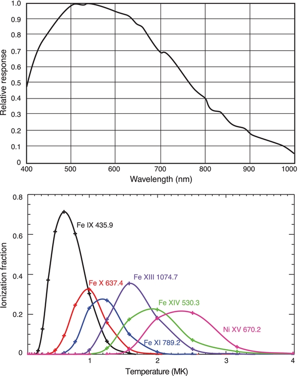
Figure 1. Top: response curve of the Atik314L detector, normalized to a maximum of 1, as a function of wavelength. Bottom: ionization equilibrium curves for the spectral lines used for the eclipse observations, calculated from CHIANTI using the Mazzotta et al. (1998) database.
Download figure:
Standard image High-resolution imageThe thermally controlled interference filters were mounted in front of the lens system. The filters were all tilted by approximately 10 to move any potential ghost images beyond the 2° field of view. This tilt resulted in a wavelength shift of the line center by no more than −0.04 nm, which was compensated for by adjusting the temperature of each filter to ensure that its bandpass was centered on the line to ±0.03 nm. Each complete optical system was adjusted with an optical collimator using a 200 mm off-axis parabolic mirror and a white light LED as a light source. Different color LEDs were used as the collimator light source for focusing the lens set-up without the interference filters. During the eclipse, the camera systems were mounted on four identical Astrophysics German equatorial mounts tracking the Sun. To optimize the data acquisition throughout totality, sequences of increasing and decreasing consecutive exposure times, varying by a factor two, were implemented. The minimum and maximum exposure times are given in Table 1.
Table 1. Characteristics of the Spectral Lines
| Spectral Line | Hα | Fe ix | Fe x | Fe xi | Fe xiii | Fe xiv | [Fe xv]* | Ni xv |
|---|---|---|---|---|---|---|---|---|
| Ionization State | Fe8 + | Fe9 + | Fe10 + | Fe12 + | Fe13 + | Fe14 + | Ni14 + | |
| λ (nm) | 656.3 | 435.9 | 637.4 | 789.2 | 1074.7 | 530.30 | 705.86 | 670.17 |
| Tmax (106 K) | 0.02 | 0.5 | 0.8 | 1.16 | 1.6 | 1.8 | 2.5 | 2.5 |
| E (eV) | 13.6 | 233.6 | 262.1 | 290.2 | 361.0 | 392.2 | 457 | 464 |
| A (s−1) | 4.41 × 10⁷ | ≈50 | 69.4 | 43.7 | 14 | 60.2 | 37.4 | 56.5 |
| I☉/I☉(500.2 nm) | 0.851 | 0.953 | 0.878 | 0.654 | 0.342 | 0.992 | 0.777 | 0.831 |
| Min. exp. t (s) | 0.002 | 0.05 | 0.05 | 0.08 | 1.05 | 0.05 | 0.05 | |
| Max. exp. t (s) | 67.62 | 28.47 | 28.47 | 21.19 | 67.40 | 28.47 | 28.47 |
Notes. E is the ionization energy relative to the ionization state immediately below, i.e., from charge state i to i + 1. A is the transition probability. I☉ is the intensity of the photosphere calculated from the Planck function, at a given wavelength, for a blackbody T of 5800 K, which peaks at 500.2 nm. The Fe xv line (given in brackets with an asterisk) was not observed but is included for comparison.
Download table as: ASCIITypeset image
3. DATA CALIBRATION
Since the sky was not absolutely clear throughout totality, images significantly influenced by clouds were not used. For the broadband white light observations, 61 out of the 89 images were selected. For the narrowband spectral line images, 20 were chosen from the Fe ix pair with the longest exposure time tmax = 14.23 s, 28 from the Fe x pair with tmax = 28.47 s, 22 from the Fe xi pair with tmax = 16.11 s, 27 from the Fe xiv pair with tmax = 28.47 s, 20 for the Ni xv pair with tmax = 28.47 s, and two exposures from Hα of 0.36 s and 1.05 s long. For the Fe xiii system, the shortest exposure time used was 8.42 s. The impact of the clouds was the strongest for the Fe ix system and the least for the Ni xv system.
The broadband white light images were calibrated using over 600 dark frames and flat-field images. For the spectral line imaging, dark frames, flat-fields, and dark frames for flat fields were taken with every camera. In particular, four dark frames with identical exposure times matching the exposure time of the corresponding eclipse image were acquired. These four dark-frames were then averaged in order to decrease the additive noise. The dark frames for flat-field images were taken with the same exposure time as the flat fields.
All seven sets of offline and online pairs of images were aligned by means of the phase correlation technique developed and described by Druckmüller (2009). This technique enables one to find the scaling factor, the angle of rotation, and the translation vector necessary to align all images with sub-pixel precision, even for images taken with different exposure times and through different narrow bandpass filters. Prior to the alignment, the images had to be corrected for the darks and the flat fields as follows: darks were subtracted from each online and offline image, as well as from the corresponding flat fields. The resulting image was then divided by the dark-corrected flat field. The online and offline images thus calibrated were then subtracted from each other.
Mathematically speaking, the approach is executed as follows. Let Ek, i denote the sequence of eclipse images and Dk, i the sequence of corresponding averaged dark frames, where the index i = 1, 2, ..., n refers to the exposure times, k = 0 refers to the continuum, and k = 1 to the spectral line. Let Fk, j denote the sequence of flat-field images and Qk, j the sequence of corresponding dark frames, where j = 1, 2, ..., m refers to the exposure times of the flats and corresponding dark frames. The final calibrated image, Li, for a given spectral line with the continuum subtracted, at exposure time i, is then given by
where w is the product of the ratio of the solar continuum in the corresponding online and offline images and the ratio of the intensity of the light source used for the flat-field panel at these two wavelengths. It is a constant nearly equal to one. The spectrum of the flat-field panel was measured for this purpose. For each spectral line, the sequence of calibrated images Li was then combined into one single 64 bit pixel−1 image with a linear scale brightness.
Since each spectral line image resulted from the combination of different exposure times, the noise parameters depend on the location within a given image. Consequently, it is not possible to characterize the noise by one single number. Furthermore, since the data were not used to calculate density and temperature, calculation of the signal-to-noise ratio is not important here and is not needed in the processed images (see Section 4). Any structure we see is actually present; the noise cannot create coherent structures.
4. IMAGE PROCESSING
With the exception of the human eye, no recording medium does justice to images of the corona obtained during total solar eclipses, because of the steep decrease of brightness and the sharp decrease in contrast between coronal structures with increasing height. To compensate for these effects in an attempt to bring out all the inherent details of coronal structures, different approaches for processing images have been developed over the years (e.g., Koutchmy et al. 1988; Morgan et al. 2006; Druckmüller et al. 2006). In this study, two techniques were applied to the calibrated images: the Adaptive Circular High-pass Filter, or ACHF, developed by Druckmüller et al. (2006) and the Normalizing Radial Graded Filter, or NRGF, developed by Morgan et al. (2006). We briefly discuss below the main differences and advantages of each technique. We note though that only the unprocessed calibrated images are used for the quantitative analyses.
The principle of the ACHF is to enhance the high spatial frequencies and to attenuate the low spatial frequencies in such a way that the resulting image is very close to what the human eye sees. The human vision is in principle a differential analyzer. That is why the highest spatial frequencies produce the majority of the visible information. This is achieved with the unsharp masking technique. Before the ACHF is applied to an image, the pixel values throughout the image are transformed into a logarithmic scale. The unsharp masks have an adaptive kernel which ensures a circular characteristic frequency at high spatial frequencies and minimizes the edge effect at the lunar limb. While the information about the absolute brightness is lost in the ACHF-processed images, the fine details, which in principle are not possible to see in the original unprocessed images, are visualized without introducing any processing artifacts. A typical range of pixel values in the eclipse images is 〈0, 106〉 and the resulting images are in 8 bit pixel−1 format, i.e., 〈0, 255〉. Without the ACHF much of the fine scale structures would remain invisible.
The NRGF removes the steep decrease of brightness by subtracting the average decreases of the radial brightness. It compensates for the decrease of the relative contrast of structures by dividing by the radial standard deviation of brightness. Full details are given in Morgan et al. (2006). This robust and simple technique preserves the large-scale shape of the corona while allowing the fair comparison of structures at different heights.
The complementarity of the two image processing techniques proved to be essential for revealing the fine details of large- and small-scale structures, and provided invaluable empirical insight into the physics of coronal plasmas. We show in a companion article (Druckmüllerová et al. 2011) how a newly developed technique, referred to as the Fourier Normalizing Radial Graded Filter (FNRGF), can improve on the NRGF by enhancing fainter structures while preserving the appearance of the corona on large scales.
5. CORONAL STRUCTURES IN WHITE LIGHT
One of the novel advantages of this eclipse experimental setup was the acquisition of broadband white light and narrowband continuum images of the corona. This complement provided two different means for exploring coronal structures as they appeared in the emission from photospheric light scattered off coronal electrons, throughout the wavelength range of the blackbody radiation, both in the wide bandpass of 400–650 nm of the RGB filters of the Canon camera and in discrete 0.5 nm bandpasses within the wavelength range of 400–1100 nm. The terms white light and continuum thus refer to images devoid of contribution from coronal emission lines. In the broadband white light image their contribution is naturally averaged out. The 0.5 nm bandpasses of the offline filters were deliberately chosen to exclude their contribution as well. The suite of continuum images also served as a valuable test of the observing conditions and the calibration process.
5.1. The Broadband White Light Image
The broadband white light image of the corona, processed with the ACHF, is shown as a negative in Figure 2. Such a display reveals the details of coronal structures better than the positive image, which is available in the online version. The moon inset shows the earthshine acquired through a combination of the different exposure times used to produce this white light image (as described earlier in Section 3). The position of the Moon corresponds to 157 s after C2, past the midway point of totality; hence, it is almost centered on the solar disk.

Figure 2.
Broadband white light negative image of the corona processed with ACHF. This negative image, with the brightest features appearing in black, yields the best contrast for visual inspection. The largest prominence is shown in red as a result of its strong Hα emission. The position of the Moon corresponds to 157 s after C2, past the midway point of totality, hence it is almost centered on the solar disk at that time. The image must be rotated by 3° counterclockwise to align it with solar north. A mirror Ritchey–Chrétien optical system (d = 203 mm, f = 1624 mm) and a Canon EOS 5D were used. (An extended version of this figure is available in the online journal)
Download figure:
Standard image High-resolution imageThe most striking features in this image are the preponderance of sharply defined ray-like structures filling the corona and expanding away from the Sun, and of arch-like structures of different scales surrounding the Sun with the exception of the polar regions. These features are labeled in Figure 3 for ease of reference. Also labeled in Figure 3 are other unusual features which are described in detail below.
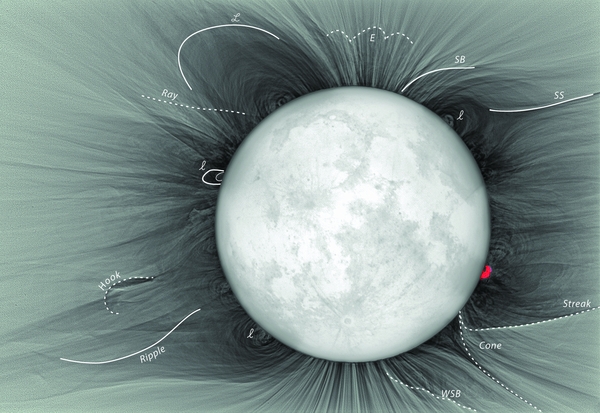
Figure 3. Same as Figure 2 with labels assigned to features, such as distinct rays, Ray, small-scale loops, l, large-scale loops, L, the streamer stalk, SS, the streamer boundary, SB, the Hook, and the enhancement E. The Ripple, the wavy streamer boundary, WSB, the Streak, and the Cone are examples of structures resulting from prominence eruptions and the passage of CMEs through the corona prior to totality, as described later in Figure 9.
Download figure:
Standard image High-resolution imageIn the polar regions, rays with very sharp edges and a range of brightnesses, commonly referred to as polar plumes, expand outward to the edge of the field of view. In addition to these plumes, there is a remarkable feature, labeled E, appearing like a shadow, centered almost dead north. It is most likely a projection of the bulge of a streamer along the line of sight. One can readily see that this could be the case from considering the streamer at the northwest, with its stalk labeled SS. Its northernmost boundary, labeled SB, is at position angle P.A. = 340°, measured counterclockwise from 0° north, while the stalk SS extends radially down to P.A. = 300°. If such a streamer were at central meridian at the time of the eclipse, its bulge could readily project up to the height of the observed enhancement E. This will become more evident when we describe the emission from the hotter spectral lines in Section 6.3.
Away from the polar regions, the corona is encircled by a complex of small, seemingly intertwined, loop-like structures, labeled l. At the resolution of this image, the smallest arches are about 1.1 R☉ in height. The overlay with the Hα emission (Figure 4) shows that prominences lie immediately below them. Overlying these smallest loops is another forest of intricate, and also seemingly intertwined, loops, labeled L, reaching heights of approximately 1.23 R☉. The largest loops extend out to heliocentric distances of 1.5–1.7 R☉, with the most evident ones appearing on the northeast. Beyond 1.2 R☉, the corona becomes dominated by a myriad of converging and diverging open field lines, in what seems to be layers of streamer-like structures populating the line of sight. Some of them have a classically shaped helmet, such as the northeast one. The orientation of others is such that they appear as different projection profiles of their three-dimensional structures onto the plane of the sky, as described earlier in connection with the streamer associated with SS. We also note the presence of rays, such as the one labeled Ray, which do not seem to be associated with any particular large-scale structure, as they seem to criss-cross the corona in arbitrary paths.
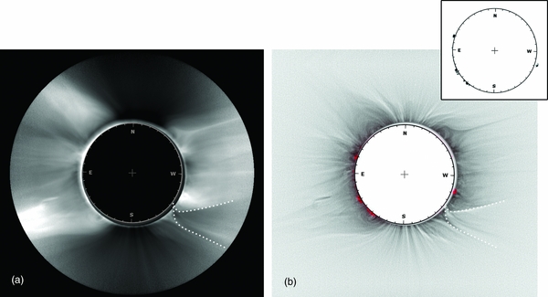
Figure 4. Fe xi associated offline image, (Fe xi)C, processed (a) with NRGF and (b) with ACHF shown as a negative. Both images have the same scale. The inset is an Hα composite from one Hα image taken at C2 + 23 s with an exposure time of 0.26 s and one at C2 + 185 s with an exposure time of 1.05 s. It shows all the prominences present around the limb throughout totality. The prominences are shown superimposed in red in (b). The grid corresponds to the location of the Sun at C2 + 23 s. The Cone labeled in Figure 3 is outlined by dashed lines.
Download figure:
Standard image High-resolution imageThere are also ripples and wave-like structures at the boundary of one streamer, labeled Ripple and WSB, respectively, which are likely the result of the passage of CMEs through the corona prior to the eclipse. This is also the case for the Streak, the Cone, and the Hook, as will be described in more detail later on.
5.2. The Narrowband Continuum Images
The continuum images, (Z)C, were processed with both NRGF and ACHF. The comparison between the two is best illustrated in Figure 4 for the same continuum image, which is  in this example. The full suite of NRGF-processed images, with the exception of (H
 , is given in Figure 5. It is worth commenting first on the main difference between the two processing techniques. The ACHF enhances small structures, namely, the high spatial frequencies. With its equal amplification throughout an image, the comparison between different parts can be readily made. The NRGF method, on the other hand, uses a variable signal amplification which depends on the intensity fall-off with increasing distance, and in latitude within a given radial band. While the amplification can theoretically converge to infinity, in reality the noise stops the amplification at some high level. Consequently, localized enhancements appear visually more amplified in the NRGF- than in the ACHF-processed images.
Figure 5. NRGF-processed offline, or continuum, images corresponding to the spectral lines shown in Figure 6. The inset grids give the position angles and correspond to the location of the solar disk at that time of totality. The Cone is outlined by dashed lines in (Ni xv)C.
Download figure:
Standard image High-resolution imageIn the comparison of Figure 4, both images have the same scale, with the ACHF shown as a negative image, as in Figure 2. The circular grid corresponds to the position of the underlying solar disk relative to the Moon at that moment of totality. It is not always at the same location since the optimal frames chosen within each bandpass, when the impact of clouds was minimal, did not necessarily correspond to the same exposure times. Although the spatial resolution of the continuum images is 65 compared to the 1'' in the white light image of Figure 2, most of the details found in Figure 2 are visible here. Since the NRGF amplifies low contrast and faint signals far from the Sun, the visual impression of coronal structures is somewhat different when compared to ACHF. For example, the large-scale structures are more evident with the NRGF, while the details of the polar regions are lost in that image. The sharp streamer stalk, SS, is very well defined in both images, so are the Streak, the outlines of the Cone, delineated by dashed lines, and the Hook. The details of the small-scale loops seen in Figure 2 are reduced in the lower resolution ACHF image and absent in the NRGF one. However, some of them appear as dark "cavities" in the latter image, as is often the case in most low-resolution white light images.
To establish the origin of the small-scale loops associated with dark cavities, we consider next the emission from prominences as seen in Hα, shown as an inset in Figure 4. The inset is a composite of two different observing times: C2 + 23 s with an exposure time of 0.26 s and C2 + 185 s with an exposure time of 1.05 s. In Figure 4(b), these prominences are shown in red overlaid on the white light corona. The prominence at the southwest, at P.A. = 250°, is the largest one as it protrudes above the edge of the Moon in Figure 2 at that time of totality. This composite shows how the intricate small-scale loop-like structures directly overlay prominences. Comparison with the NRGF-processed image (a) further shows how all the prominences lie at the base of the large-scale structure, or bulges, of streamers. We also note that the strong Hα emission from the prominences, coupled with the varying sky conditions, limited the choice of useable Hα exposure times to 0.26 and 1.05 s. With these exposure times the only detected Hα emission was from prominences. Therefore, we cannot conclude from these observations whether other traces of Hα emission were present in the corona.
The full suite of continuum images shown in Figure 5 was also very useful for testing the quality of the optical systems and for gauging the impact of the observing conditions on the different wavelengths, if any. When taking into account the detector response of both Atik (Figure 1) and PIXIS cameras as a function of wavelength, the transmission curves of the filters, and the approximately blackbody curve of the photospheric radiation, the intensities in all these white light images were found to be comparable. In particular the sharp streamer stalk, SS, the Streak, the outlines of the Cone, delineated by dashed lines in  , and the Hook readily stood out in all images with the exception of
  and
and  . These exceptions are attributed to the impact of the sky conditions, which was strongest at the (Fe ix)C wavelength, as is evident from the much higher noise level beyond 2 R☉ in comparison with the other continuum images, and to the very low detector response at
  (see Figure 1).
Finally we point out that the  image, centered at 434.8 nm, was such that it captured some Hγ emission at 434.0 nm at the 10% level within its bandpass. Consequently, emission from the cool prominences appeared in that bandpass. The subtraction process of offline from online images then led to negative values at those locations, seen as black in the Fe ix image of Figure 6, which will be described next.
Figure 6. NRGF-processed spectral line images resulting from the subtraction of the offline from the online images. The dashed lines outline the boundaries of the Cone-shaped CME, which traversed the corona prior to totality and left a marked void in Fe ix, Fe xiv, and Ni xv. See also Figure 9.
Download figure:
Standard image High-resolution image6. CORONAL STRUCTURES IN EMISSION LINES
6.1. Identifying Coronal Structures at Different Temperatures
The suite of selected spectral lines covered the temperature range from 4 × 10⁵ K to 3 × 10⁶ K, as demonstrated by the ionization equilibrium curves shown in the lower panel of Figure 1. Since the peaks of their ionization curves are well separated, this choice provided a relatively clear identification of the underlying electron temperature in the observed emission without having to recur to any modeling, or differential emission calculations, such as is the case for most current space-borne EUV observations (e.g., EIT, STEREO, and SDO). For example, any structure observed only in Ni xv would have a temperature at its peak ionization fraction, Tmax = 2.5 × 10⁶ K, but not more than 3 × 10⁶ K. Beyond that temperature, the ionization fraction of Ni xv drops to less than 10% of its peak. At Tmax(Fe xiv) emission from both Fe xiii and Ni xv should be present. At Tmax(Fe xiii), emission from Fe xiv could be present but not from Ni xv. Moving to lower temperatures, at Tmax(Fe xi), the ionization fraction of Fe x and Fe xiii is down by almost a factor of two, hence it would be possible to see structures in Fe xi only, if the electron temperature were so narrowly distributed. On the other hand at Tmax(Fe x), Fe xi should be detected, while Fe ix, whose ionization fraction is down by more than a factor of two, would be much weaker. At Tmax(Fe ix) emission from that spectral line only would be visible.
To expose the temperature in the large-scale and small-scale density structures, the eclipse spectral line images were processed with both NRGF (Figure 6) and with ACHF (Figure 7). As in the comparison of the continuum images, here too the two processing approaches yield different features. Since the NRGF reveals faint features at large radial distances, secondary ghost images created by internal reflections in the optics in some filters, despite the care taken to tilt the filters, appeared enhanced relative to the background in NRGF but were absent in the ACHF. This was the case for the Fe xi online image, the Ni xv online image, the Fe xiii offline image, and consequently the Fe xiii line image when the offline was subtracted from the online image. However, since these ghost images have less than 0.1% of the intensity of the primary image, and since their position is known, their potential effect and corresponding uncertainty can be calculated so as not to interfere with the coronal line emission diagnostics.
Figure 7. Same spectral line images as in Figure 6 processed with ACHF and shown as negatives. The Cone is also given by the dashed lines in all panels.
Download figure:
Standard image High-resolution imageInspection of both Figures 6 and 7 shows that the strongest and most radially extended emission appears in Fe x, Fe xi, and Fe xiv, while the Fe ix, Fe xiii, and Ni xv images show the weakest and least extended emission. Furthermore, the small- and large-scale structures are not the same in the different spectral lines. There is also a distinct demarcation in the appearance of the corona between the cooler lines of Fe ix, Fe x, and Fe xi formed below 1.2 × 10⁶ K, and the lines formed above 1.8 × 10⁶ K, namely, Fe xiii, Fe xiv, and Ni xv. This demarcation is especially striking in the large-scale structures of the NRGF-processed images. We consider next the weaker emission, and then proceed to a discussion of the temperatures associated with the stronger emission.
6.2. Investigating the Weaker Emission of Fe ix, Fe xiii, and Ni xv
The observed weakness of the Fe ix emission can be attributed, in part, to its particular transition mechanism. While all other emission lines are caused by magnetic dipole transitions to the ground state of their respective ion, the Fe ix emission is a metastable magnetic dipole transition between two high lying states (3p53d1D2 to 3p53d3F2) of Fe8 +. Therefore, there is essentially no radiative excitation of this line, as radiative excitation out of the ground state would require significant incident intensity at 21.9 nm. Furthermore, the branching fraction into Fe ix 436 nm from the upper level is only 22%, as this forbidden transition competes with other forbidden transitions from the same upper level to ground and various lower lying excited states. Consequently, the population of the upper 1D2 state is diminished and emission from this spectral line is expected to be weak. Another factor potentially contributing to this weakness is the paucity of coronal density structures at the peak of the ionization fraction of Fe8 + around 6 × 10⁵ K.
Despite its weakness, the striking characteristic of the Fe ix NRGF-processed images is the presence of very sharply delineated structures extending out to at least 2 R☉. One example is the appearance of "negative" (black) emission at the location of some prominences, for example at P.A. = 75°, 120°, 250°. Although caused by emission from Hγ in the bandpass of the offline filter, thus becoming negative when subtracted from the online as noted earlier, the resulting sharply delineated prominences prove that the quality of the optical system was excellent and that the alignment of the offline and online Fe ix images was such that the fine structures are indeed real. Most striking among these features are the fine details of the southeast streamer, the Streak, and the northern boundary of the northwest streamer with its stalk, labeled SB and SS, respectively, in Figure 3. The Hook is very faint but sharply delineated. There is also one dim low-lying loop at the base of this streamer, appearing as an absorption feature. A dashed line has been drawn over the Streak, and another one as a curve below outlining one boundary of the southwest streamer. The relevance of the cone-shaped region defined by these two curves, and labeled Cone in Figure 3, will become more apparent in Section 6.4 when we consider the passage of a CME in that location prior to the eclipse observations. Although polar plumes appear clearly in the south, but less so in the north, their structures are not as sharply delineated as the other structures described above. The impression from the corresponding ACHF-processed image is that the emission is more diffuse and fills the corona when compared to the NRGF-image. In both images, however, no Fe ix emission appears in the Cone. Based on these two differently processed Fe ix images, it is clear that some coronal emission does indeed exist in the temperature range where Fe ix can be ionized. A tighter constraint on the temperature range of the Fe ix observed structures can be set once we consider emission from Fe x, as will be discussed in the following section.
We consider next the Fe xiii emission. The low count rates, which resulted in a higher additive noise and a lower image quality, are a direct consequence of the 100 times weaker response of the detector at 1074.7 nm compared to its response at 530.3 nm, as noted earlier when discussing the corresponding continuum images. Although the scattering radiation from the photosphere at 1074.7 nm is 3× weaker than at 530.3 nm (see Table 1), the radiative scattering cross section is more than an order of magnitude larger than at 530.3 nm, so that visually the coverage of this emission is nearly as extended as Fe xiv and seemingly comparable to Fe xiv, albeit with lesser well-defined details. We note that the ionization fraction of Fe xiii is equal to that of Fe xi at T = 1.35 × 10⁶ K and to Fe xiv at 1.9 × 10⁶ K. It is therefore likely that the observed Fe xiii emission, despite the low detector response and the lower scattering radiation from the photosphere at that wavelength, is a reflection of the presence of coronal structures at the peak ionization temperature of Fe xiii.
The other observed weak emission in the corona is from Ni xv. This is evident in both NRGF- and ACHF-processed images. In comparison with Fe ix, the emission appears much more diffuse but has an equally limited radial extent. The weaker observed Ni xv emission is likely due to a factor of 20 lower Ni abundance compared to Fe. Although the detector response (see Figure 1) at 670.2 nm is 25% lower than at 530.3 nm, the range of exposure times should have been sufficient to unveil this emission to large distances if it were present. Indeed, the corresponding continuum emission (Ni xv)C is indistinguishable from (Fe xiv)C (see Figure 5). From the ionization fraction curves shown in Figure 1, it is clear that Ni xv emission should be present whenever Fe xiv emission is detected. Since no Ni xv emission was observed without an Fe xiv counterpart, we conclude that the overall weakness of the Ni xv emission most likely reflects the absence of coronal structures at electron temperatures Te > Tmax(Ni xv). The low Ni abundance compared to Fe is another potential contributing factor.
6.3. Coronal Structures in the Strongest Lines of Fe x, Fe xi, and Fe xiv
The details of the most prominent and puzzling coronal structures labeled in Figure 3 are best described in the strongest emission of Fe x, Fe xi, and Fe xiv, in both the NRGF- and ACHF-processed images. Based on their ionization fraction curves, one would expect the emission from Fe x and Fe xi to be very similar to, but not necessarily the same as, Fe xiv.
Features, labeled l, refer to low-lying loops at the base of streamers best seen in the white light image of Figure 2. A large number of them stands out on the east limb in both Fe x and Fe xi in Figure 6, overlying cavities centered at P.A. = 75°, 105°, 125°, and 145°. The latter is very prominent in Fe ix. In contrast, the loops at 35°, 145°, and 315° are dominated by hotter material.
Large-scale loops, like the one labeled L in Figure 3, dominate the streamer centered at P.A. = 35° in the NRGF-processed Fe xiii and Fe xiv images of Figure 6. They are faint in the Ni xv image. Their edges are visible in Fe x and Fe xi, mostly in the ACHF-processed images.
The thinly defined structure labeled Hook in Figure 3 is prominent in Fe x and more so in Fe xi. It appears as a complex structure connected to the solar surface in both NRGF- and ACHF-processed images. The fainter structures between the Hook and the solar surface appear more like a void in the NRGF-processed Fe xiii, Fe xiv, and Ni xv images. But their ACHF counterparts show intricate features, implying that hotter structures are present, albeit rather faint when compared to their immediate surrounding.
Twisted structures, such as the Ripple, pervade the NRGF-processed Fe x and Fe xi images. The wavy streamer boundary, labeled WSB in Figure 3, is another example of a ripple effect. As will be discussed later in Section 6.4, ripples are most likely the byproduct of the passage of CMEs through the corona and are best seen in emission around 106 K.
Structures in the polar regions are seen in the NRGF-processed images only in Fe ix and Fe x, and only in the south pole, but they are prominent in Fe ix, Fe x, and Fe xi in both polar regions in the ACHF-processed images (Figure 7). Curiously, some Fe xiv emission appears between P.A. = 350° and 360°. As discussed earlier, upon closer examination of the details of the fine scale structures in white light (Figure 2) it becomes evident that this emission is due to the bulge of a streamer in the foreground or background, or along the line of sight. Such a bulge would have a shape very similar to the streamers adjacent to the polar coronal hole but seen in projection from 90° away from the central meridian in the plane of this image. This is also the case for the south polar region with faint rays appearing in Fe xiv.
The Streak, which appeared as a remarkably sharp boundary in the white light image of Figure 2 extending outward from P.A. = 240°, is delineated by a dashed line in both the NRGF and the ACHF images, defined by the Fe ix emission. The Streak also shows up as a very sharp boundary in Fe xiii, Fe xiv, and Ni xv, but, curiously, is extremely faint in Fe x and is absent in Fe xi. Another boundary, delineated by a dashed line south of it, also determined from the Fe ix emission, and present in the white light and continuum images, originated at almost the same latitude at the Sun. These two dashed lines form the Cone. The Streak is likely to represent a very thin sheet with a two-temperature structure: very cold (Fe ix) on one side, and very hot (Fe xiii, Fe xiv, and Ni xv) on the other.
To further proceed with the identification of coronal structures with well-defined electron temperatures, overlays of the strongest emission lines from the ACHF-processed images are shown in Figure 8. Fe x is shown in red and Fe xiv in green, following the true colors of these spectral lines. Fe xi is shown in cyan. The overlay of Fe x and Fe xi, two lines which are very close in their peak formation temperature, is shown in Figure 8(a). Since the images do not have an absolute calibration, neutral gray is chosen as a reference ratio of equal Fe x and Fe xi average intensities. Fe x and Fe xiv, which vary by a factor of two in their peak ionization temperature, are shown in Figure 8(b). When Fe x is dominant the color is red, while the dominance of Fe xi appears as cyan. The same amount of Fe x and Fe xiv yields yellow, which represents a reference ratio between the intensities of these two lines. When Fe x is dominant, the color is red. The dominance of Fe xiv appears as green.
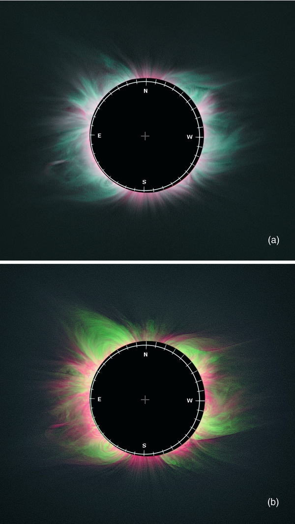
Figure 8. (a) Overlay of Fe x (red) and Fe xi (cyan). The same intensity in both lines produces a neutral gray. Red indicates a dominant Fe x emission while cyan indicates the dominance of Fe xi. (b) Overlay of Fe x (red) and Fe xiv (green). The same amount of these colors is yellow; red is when Fe x dominates and green is when Fe xiv dominates.
Download figure:
Standard image High-resolution imageAlthough the peak ionization temperatures of Fe x and Fe xi are very close (see Figure 1), the overlay of Figure 8(a) shows a clear distinction in the emission from these two lines. The poles are dominated by Fe x emission, while the rest of the open field lines in the corona are biased toward Fe xi. On the other hand, the overlay of Figure 8(b) yields a clear view of the demarcation in temperatures between open and closed magnetic structures in the corona. The large-scale loops are dominated by hot plasma (Fe xiv), while the expanding open structures are dominated by cool plasma (Fe x). These observations confirm the earlier results of Habbal et al. (2010c) who showed that the base of streamers are the hottest plasmas in the corona, forming shrouds around prominences, while the ubiquitous open field lines are dominated by emission from the cooler lines. The overlay of Fe x and Fe xiv emission in Figure 8(b) also makes it very clear that emission from plumes in the south polar region is dominated by Fe x emission with faint Fe xiv emission interspersed with it. In the north polar region there is marked diffuse Fe xiv emission overlying the streamlined Fe x plumes. These eclipse observations thus provide uncontroversial evidence for the occasional contamination of the polar regions by hot material along the line of sight. Hence they resolve a long-standing dilemma associated with the occasional appearance of Fe xiv emission in coronagraph observations over the poles, and provide conclusive evidence supporting Esser et al.'s (1995) statement that "... much of the temperature variations seen in the coronal holes are due to contributions along the line of sight [from the background]" (p. 19836).
Finally, we note that the Cone and the Streak clearly stand out as sharp boundaries in Figure 8(b), but are totally absent in Figure 8(a). Another example of a sharp boundary is the Ripple in Figure 8(b) clearly delineating the transition between the cool Fe x emission in the south pole and the neighboring streamer. It is not apparent as such in Figure 8(a).
6.4. The Impact of CMEs on Coronal Structures
To establish the origin of the Hook, the Streak, and the Cone, we consider next the SOHO/EIT Fe x 17.1 nm emission and the SOHO/LASCO-C2 white light coronagraph observations preceding and coinciding closely with the time of the eclipse observations, shown in Figure 9.

Figure 9. (a)–(c) Time sequence of SOHO/EIT Fe ix/x 17.1 nm emission. The arrow in the corona points to the large eclipse prominence. (d)–(f) Time sequence of SOHO/LASCO-C2 white light images. (g) Composite EIT, Fe x 637.4 nm, and LASCO-C2, with the passage of a cone-shaped CME (as outlines by the dashed lines), most likely due to a prominence eruption identified by the disk arrows in panels (a)–(c). This CME left the Cone and Streak (see Figure 3), with their corresponding extension in LASCO-C2 (see the two arrows), as delineated by the dashed lines. The circles in (a)–(c) and (g) identify the prominence eruption that ended up as the Hook. An animation of the LASCO-C2 time sequence is available in the online journal.(An animation of this figure is available in the online journal.)
Download figure:
Standard image High-resolution imageThe sequence of three EIT images, given in the top panels, shows two erupting prominences. The largest of the two, shown encircled, is at the southeast limb centered at P.A. = 110°. It had practically disappeared from the EIT field of view by 07:19 UT on July 11. On the southwest limb, shown by the arrow on the disk, another much smaller prominence had also disappeared by that time. A time sequence of LASCO/C2 images, with four images given in the lower panels, the last of which being a composite of EIT and the Fe x eclipse image, shows that there were two CMEs accompanying the disappearance of these prominences. The encircled one was less dramatic than the one on the southwest which led to a spectacular cone-shaped CME.
The Hook observed throughout the eclipse starting at 18:47 UT was most prominent in Fe x and Fe xi. Its position angle and its shape strongly suggest that it is the leading edge of the encircled very large prominence at the east limb. The Fe xi image indicates that it remained attached to the solar surface with intricate structures appearing between the leading edge (the Hook) and the solar surface. From the time difference between its disappearance at 07:19 UT on July 11 in the EIT field of view, and its observed height in the eclipse images, an average rising speed of 15 km s−1 can be inferred. The unique contribution of these eclipse observations is that a temperature of about 106 K can be assigned to its leading edge and to the intricate underlying threads extending down to the solar surface, since best seen in Fe x and Fe xi.
The evolution of the cone-shaped CME is shown in the LASCO/C2 frames preceding and almost coinciding with the end of the eclipse. This CME has two very distinct sharp boundaries (see also movie available in the online version). The composite of EIT and Fe x eclipse image (panel g) shows that the Streak which is dark in Fe x coincides remarkably well with its northern edge. Its lower boundary also has a counterpart in the Fe ix eclipse image, albeit not as striking as the streak in white light and the other lines, and would not have been necessarily singled out. These two boundaries converge through a sharp C-shaped curve that intercepts the solar disk at P.A. = 230°, which is the position angle of the east-limb prominence seen in the EIT image above. Interestingly this cone-shaped enclosure is best seen in the NRGF-processed Fe ix and Ni xv image, with the streak bright in Fe ix only (see Figure 6).
These two examples provide the best evidence for the impact of eruptive prominences and CMEs on the density structures in the inner corona, i.e., 1–3 R☉, a region that is not imaged by any other instrument. What these observations also yield is a temperature marker for the sharp boundaries that they create. Although prominences are the coolest material in the corona, surrounded by the hottest loops there, these observations indicate that their temperature signature changes dramatically as they expand through the corona: the temperature of the leading edge of the prominence reaches 106 K, while the bulk of the volume of the CME associated with the prominence eruption consists of a complex of coronal material with a mixture of hot and cool material. The example of the cone, however, yields an original example of a cool void (around 106 K) created by the passage of the CME, with a very thin boundary in the form of a two-temperature sheath, as determined from the Fe ix and Fe xiv emissions.
7. IMPORTANCE OF THE RADIATIVE COMPONENT OF CORONAL FORBIDDEN LINES
The white light and multi-wavelength images of the corona, described above, provide ample evidence for the importance of these forbidden lines for exploring the thermodynamic properties of coronal density structures. The suite of spectral lines selected for these eclipse observations showed how, despite the complexity of coronal structures, distinct temperatures could be assigned to them in an unambiguous manner.
In general, emission lines have two main components contributing to their intensity. One component results from collisional excitation due to collisions between ions and electrons. The other radiative component is due to excitation of ions by the high intensity of light from the solar disk. Since the solar disk has practically no emission short of 100 nm, the EUV counterparts to the coronal forbidden lines, e.g., Fe ix 17.1 nm, Fe x 17.4 nm, and Fe xiv 27.5 nm, will only have a collisional component as will be demonstrated next, while the coronal forbidden lines observed from the ground, with the exception of Fe ix 436 nm, have both components.
The collisional and radiative components have distinct properties. The intensity of the collisional component is the line of sight of the integral of emission due to collisions between ions and electrons. It is therefore proportional to the product of ion and electron density, and a collisional rate factor dependent on the local electron temperature. Its dependence on the ion and electron density product implies a sharp fall-off with radial distance. The collisional rate factor is a much weaker distance varying term. The radiative component is the line of sight integral of emission due to radiative excitation of ions by the high intensity of light from the solar disk. It is therefore proportional to the ion density times the disk intensity at the appropriate wavelength. Hence, its radial fall-off is a lot shallower than the collisional component. Consequently, the radiative component of coronal forbidden lines enables the tracking of coronal emission to much larger distances than their EUV counterpart. This is essential for understanding the evolution of the coronal magnetic field with distance from the Sun, in particular when an ambiguity exists for establishing which field lines remain tied to the Sun through large-scale loops, and those that escape from the Sun with the solar wind flow. We show next how these two components can be separated observationally.
7.1. Comparison of Fe x 637.4 nm with Proba2/SWAP Fe x 17.4 nm
The availability of observations of the Fe x 17.4 nm line by the Proba2/SWAP instrument during the eclipse provided an ideal tool for illustrating the importance of the radiative component in the coronal forbidden lines by comparing emission from this EUV line with its Fe x 637.4 nm counterpart. The invaluable importance of this comparison is twofold: (1) it offers a direct comparison between the behavior of a collisionally excited spectral line (17.4 nm) and one (637.4 nm) where radiative excitation dominates collisional excitation beyond a given heliocentric distance and (2) it provides a test for the accuracy with which the acquisition, calibration, alignment, and composing of the online and offline eclipse images were executed.
Shown in Figure 10 is the SWAP Fe x 17.4 nm image (a), the Fe x 637.4 nm eclipse image (b), and a composite of the solar disk imaged in 17.4 nm with the corona in 637.4 nm (c). Here, the brightness of the 637.4 nm coronal image was calibrated against the innermost corona in 17.4 nm, thus rendering the transition between the two images invisible. This would not have been possible had there been an inherent difference between the two. To illustrate the point, all three images are shown without any structure enhancement. Images in panels (a) and (b) are displayed in a logarithm brightness scale, while panel (c) is displayed in a brightness scale with increased contrast in the dark part of the image. The similarity between the two images close to the Sun becomes even more remarkable with the realization that they were taken with two different instruments, under different observing conditions with one from space and the other from the ground. The extent of the 637.4 nm in the corona, compared to the extent of the 17.4 nm, is striking. Most noticeable is the fact that the Hook, which is so prominent in 637.4 nm, is very weak in 17.4 nm.
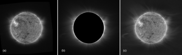
Figure 10. Comparison of the Proba 2/SWAP Fe x 17.4 nm emission (a) with the Fe x 637.4 nm emission observed at the same time during the eclipse (b). (c) is a composite of the Fe x 17.4 nm disk image with the Fe x 637.4 nm coronal image. The brightness of the coronal image was calibrated against the innermost corona in 17.4 nm. None of the images are processed. (a) and (b) are displayed in a logarithmic brightness scale. (c) is displayed in brightness scale with increased contrast in the dark part of the image.
Download figure:
Standard image High-resolution imageA close-up of the details of the northwest quadrant of the corona is shown in Figure 11. The first two images are the same 17.4 nm SWAP image, with the solar disk covered by a black disk in the middle panel. The right image is the 637.4 nm emission. In the middle and right panels, the 17.4 and 637.4 nm images are indistinguishable. The only exception is the marked radial extent of the 637.4 nm image further out in the corona compared to 17.4 nm, especially in the polar region. This comparison is a classic illustration of the difference between the dominance of radiative excitation, such as in Fe x 637.4 nm, with only collisional excitation, such as in Fe x 17.4 nm.
Figure 11. Detailed comparison of the Proba 2/SWAP Fe x 17.4 nm emission with the Fe x 637.4 nm in the northwest section of the corona. In the middle panel, Fe x 17.4 nm is shown as a simulated eclipse with the solar disk covered by a black circle. The difference between the 17.4 and 637.4 nm images is the marked radial extent of the 637.4 nm image compared to 17.4 nm, especially in the polar region.
Download figure:
Standard image High-resolution imageAnother visualization of the effect of radiative excitation by photospheric radiation for the Fe x 637.4 nm is shown in Figure 12. This color overlay of the two lines, in the quadrant shown in Figure 11, shows red for Fe x 17.4 nm and cyan for Fe x 637.4 nm. We note that the vastly different average lifetimes of their excited state are 5.56 × 10⁻¹² s and 1.44 × 10⁻² s, respectively. Because of the use of complementary colors, neutral gray represents a 1:1 ratio. The cross indicates the position where the ratio was defined as 1:1. This location was chosen in a dense coronal region where the collisional excitation (which is the only excitation process for 17.4 nm) is dominant for 637.4 nm. Note that the actual ratio (in photons) of the 637.4 nm to 17.4 nm line intensities under these conditions is 0.82 (CHIANTI version 6.0). The colors thus reflect the relative ratios between the intensities of these two lines. The appearance of blue indicates where the radiative component of 637.4 nm dominates over the collisionaly excited emission from 17.4 nm line.
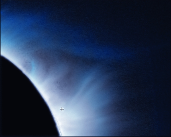
Figure 12. Visualization of the Fe x 637.4 nm radiative excitation by the photospheric emission. The color image consists of two components: red is the Fe x 17.4 nm line observed by Proba 2/SWAP, which has an average life time of excited state 5.56 × 10⁻¹² s. Cyan is Fe x 637.4 nm which has an average lifetime of excited state of 1.44 × 10⁻² s. Because of the use of complementary colors, neutral gray represents a 1:1 ratio. Color then represents the ratio between the intensities of these two lines. The cross indicates the position where the ratio was defined as 1:1, chosen in a dense coronal region where the collisional excitation, which is the only excitation process for 17.4 nm, is dominant for 637.4 nm. Blue indicates a dominance of 637.4 nm over the collisionally excited 17.4 nm line, i.e., when the radiative component of the 637.4 nm emission becomes dominant.
Download figure:
Standard image High-resolution imageAnother byproduct of this comparison is how fast collisional effects decrease with radial distance in different coronal structures. The 637.4 nm emission (blue) dominates in the polar region very close to the coronal base and along the boundary of the adjacent streamer beyond 1.1 R☉. This implies that the density gradient is very steep there leading to a sharp drop in the 17.4 nm intensity, while the radiative component of 637.4 nm secures a detectable emission. On the other hand, in the densest part of the streamer, the 17.4 nm emission extends further away from the Sun than in the poles, a reflection of the shallower gradient of the density there compared to that in the polar region.
To summarize, the advent of contemporaneous observations in two Fe x lines, namely, 637.4 nm and 17.4 nm, yielded a unique opportunity to compare the behavior of a collisionally excited spectral line (17.4 nm) and one (637.4 nm) where radiative excitation is significant. The strong, often indistinguishable, similarity between the 17.4 and 637.4 images in the densest coronal structures lends very strong support to the reliability with which the acquisition, calibration, and alignment of the online and offline eclipse images were executed. The extent of the 637.4 nm emission beyond emission from the 17.4 nm line yields a direct proof for the unequivocal advantage of the coronal forbidden lines for exploring the radial extent of structures in the inner corona.
7.2. Transition from Collisional to Radiative Excitation
The comparison between the forbidden Fe x line and its ultraviolet counterpart, described above, could in principle be used to identify the radial distance where the transition from a collision dominated excitation to a collisionless one occurs, i.e., when the radiative component takes over. Such a transition is important for establishing the distance beyond which the frequency of charge exchanges in the corona drops significantly, thus leading to the so-called freezing-in distance of the charge states (see Hundhausen 1968).
As illustrated above, such a comparison existed only for the Fe x line. However, we show next how this identification can be made for all the observed forbidden lines by taking the ratio of the spectral line intensity to the intensity of the corresponding continuum. This approach was first demonstrated by Habbal et al. (2007a).
Simply stated, the collisional component depends on the product of the electron, ne, and ion, ni, densities, i.e., proportional to neni, while the radiative component is proportional to ni only. On the other hand the white light is directly proportional to the electron density ne. By taking the ratio of the spectral line to the continuum, the dominance of the collisional component translates into a term that is proportional to the ion density, and hence drops very sharply with distance. When the radiative component is dominant, the ratio of spectral line intensity to white light is proportional to the ratio of the ion to electron density. If the two have the same gradient, then the ratio should be flat. Any difference in gradients should be manifested as either an increasing or a decreasing ratio with distance depending on whether the ion density lags behind the electron density in its decrease with distance or decreases faster.
Four examples of such ratios are shown in Figure 13 for different structures in the corona. The background image is the negative of  processed with the ACHF. The concentric circles at intervals of 0.25 R☉ merely serve as a guide. The four black lines on the inner white disk give the position angles at which the intensities were measured along radial traces. P.A. = 392 goes through the northeast streamer. P.A. = 1812 passes through the Hook. The trace at P.A. = 1812 passes through the south pole and the trace at P.A. = 3567 extends outward in the north pole intercepting the enhancement E detected in Fe xiv. The corresponding plots of line to continuum intensity ratios are shown in the four panels labeled with their respective P.A. values, and plotted out to 2.6 R☉, the edge of the field of view of the image shown above. The ratios were calculated for the strongest observed spectral lines: Fe x (red), Fe xi (cyan), and Fe xiv (green).

Figure 13. Top:  ACHF-processed image, with concentric circles at intervals of 0.25 R☉. The ratios of line to continuum intensities are plotted in the four panels below, as a function of height along a radial line at position angles 39.2, 107.1, 181.2, and 3567, marked by the black lines on the disk in the image above. The ratio plots are for Fe xiv (green), Fe xi (cyan), and Fe x (red). The localized enhancement E in the Fe xiv ratio is detected at P.A. = 3567 between 1.25 and 1.5 R☉. The Hook causes an enhancement in the Fe x and Fe xi ratios, centered at 1.75 R☉, at P.A. = 1071.
Download figure:
Standard image High-resolution image
The scan through the center of the northeast streamer (P.A. = 392) provides clear evidence for the transition from collision to radiative dominance for the Fe x and Fe xi lines, which occurs around 1.25 R☉. Beyond this distance the ratio flattens. Note that the Fe x signal becomes noisy past 2 R☉, while the Fe xi line remains very strong. For Fe xiv, this transition is clearly complete by 2 R☉, past a small bump between r = 1.5 and 1.75 R☉. In referring to the third concentric circle in the image above, this bump coincides with the top of the bulge of the streamer, often referred to as the cusp. This bump is an indication of a localized enhancement in the Fe13 + ion density relative to the electron density, very likely associated with the trapping of these heavy ions in the underlying closed magnetic structures.
The second example at P.A. = 1071 is a scan through the Hook that coincides with the top of an eruptive prominence. As noted earlier, the Hook was visible only in Fe x and Fe xi. This is evident here from the bump that appears between 1.5 and 2 R☉. In this example too, the transition occurs around 1.25 R☉ for both spectral lines. The Fe xiv ratio, on the other hand, shows a very different behavior, with two small and consecutive bumps, the first starting at the inner boundary and ending at 1.25 R☉, and the second following immediately, and ending at 1.65 R☉. Going back to the fine details of Figure 2, it is clear that these two bumps correspond to the intersection with underlying complex arch-like structures close to the Sun.
The third example over the south pole, P.A. = 1812, shows a transition at 1.5 R☉ for Fe x and Fe xi. The Fe xiv ratio increases steadily close to the Sun, but then flattens around 1.3 R☉. It is not clear if this is a consequence of hot material intercepting the line of sight either in front or behind the plane of the sky.
The fourth and final example is from the north pole at P.A. = 3567. The transition for Fe x and Fe xi occurs at 1.5 R☉, the same location as for the south pole. Fe xiv, however, shows a bump a little before 1.25 R☉ and expands to 1.5 R☉. This is further supporting evidence for the slight enhancement, E, seen in the white light emission (see Figure 3), and correspondingly in Fe xiv as described earlier. Such an enhancement in the Fe xiv intensity was attributed to the interception of the bulge of a streamer along the line of sight, which is quantitatively supported here by the ratio plots.
In summary, the transition from the collisional to the radiative component seems to occur consistently for Fe x and Fe xi at the same radial distance around 1.25 R☉. Such a transition in the hotter line of Fe xiv is harder to determine as reliably, since it is often unavoidably contaminated by closed magnetic structures along the line of sight below 1.75 R☉ in the examples of this eclipse.
8. SUMMARY AND CONCLUSIONS
The comprehensive wavelength coverage of the 2010 July 11 eclipse observations confirmed earlier eclipse findings that the solar corona has a clear two-temperature structure. The open/expanding field lines are characterized by electron temperatures near 1 × 10⁶ K, while the hottest plasma around 2 × 10⁶ K resides in the bulges of streamers. The first images of the corona in Fe ix and Ni xv show that very little coronal plasma is at, or below, 5 × 10⁵ K and above 2 × 10⁶ K.
The passage of two CMEs through the corona a few hours prior to the eclipse observations provided a unique opportunity to witness their impact on coronal structures. One CME left clear ripples best seen in the emission from the cooler lines of Fe x and Fe xi with a temperature of 106 K. Another CME left a clearly defined void in the shape of a cone in emission from the coolest line of Fe ix and the hottest line of Ni xv. Hence, although the 2010 and earlier eclipse observations continue to provide ample evidence that the bulges of the streamers confine plasmas around 2 × 10⁶ K, the envelope of CMEs resulting from the eruption of filaments at the base of streamers are much cooler with an electron temperature closer to 106 K.
Another important contribution of these eclipse observations is the evidence of incredibly intricate structures in the corona, especially prominent in the high-resolution white light images which revealed layers upon layers of ray-like structures and loop-like structures, covering a very broad range of sizes, along the line of sight. While most structures in the 1'' resolution white light image could be accounted for in the spectral line observations, some isolated rays, such as the one labeled Ray in Figure 3, had no signature in any of the emission lines, most likely due to their lower spatial resolution.
The spectral line observations yielded a distinct electron temperature label to all the intricate structures observed in the corona. In particular, these observations make it clear that the hot bulges of streamers can be readily present along the line of sight over polar regions and can thus seriously bias the inference of not only the electron temperature there, but also the electron density. These observations emphasize the importance of coupling polarized white light observations, whether with coronagraphs or eclipses, from which electron densities are often inferred, with high-resolution spectral line observations. It is also clear that the complexity of structures in the inner corona is the source of the shortcomings of models which try to predict the evolution of the magnetic field from the solar surface outward into interplanetary space.
The most widely used spectral lines for coronagraphic observations, namely, Fe x and Fe xiv, remain quite important. However, the sequences of eclipse observations starting in 2006, which first discovered the importance of the Fe xi line, have now proven that Fe xi should be included in any coronagraphic observation. It is one of the strongest lines in the corona as it reflects the dominant electron temperature of expanding structures, and hence is optimal for tracing them.
The diagnostic capabilities afforded by coronal forbidden lines is a direct consequence of the dominance of the radiative component in their excitation, thus enabling the detected emission to extend to 3 R☉. The fortuitous occurrence of Fe x 17.4 nm observations from space by Proba2/SWAP provided an ideal opportunity for the comparison of emission from a coronal forbidden line, namely, Fe x 637.4 nm, with a space-based EUV line, from the same upper state of the same charge state. Comparison of the emission from Fe x 17.4 nm and 637.4 nm provided the first textbook example of the role of radiative excitation in the radial extent of coronal emission beyond the contribution from its collisional component. It is precisely this property that has also enabled the discovery of magnetic structures which foster localized enhancements of heavy ion densities relative to that of the electrons, hence their abundances. Interestingly, such localized enhancements are also a function of the electron temperature.
We end by noting the rather ironic finding that eclipses continue to provide invaluable opportunities for probing coronal plasmas, unfortunately not available, at present, with any space-borne observatory. While the power of the EUV wavelength range is unquestionably essential for observations of the finest details of the spatial and temporal behavior of magnetic structures very close to the solar surface, i.e., below 1.5 R☉, as recently demonstrated by the spectacular results from the Solar Dynamic Observatory (SDO), it seems that the only way to probe the most critical region of the corona, namely, the first 1–2 R☉ above the solar surface, is with the coronal forbidden lines. There is nothing else at present that can match them.
The eclipse observations were made possible by funding from NASA Grants NNX08AQ29G and NNX07AH90G, and NSF grant ATM 08-02520, to the University of Hawaii, NSF grant NSF-AGS-0450096 to Bridgewater State University (M.A.), and NSF grant ATM-0801633 to Appalachian State University (J.S). Partial support for the work of M. Druckmüller was provided by grant 205/09/1469 of the Czech Science Foundation. This eclipse expedition to Tatakoto would not have been made possible without the creative resourcefulness and relentless support of the administrative team at the Institute for Astronomy (IfA), namely, Chris Kaukali, Faye Uyehara, and Lauren Anzai; and the fantastic response and support from John Bell (Air Tahiti), Francois Dantzer (atoll of HAO), Heifara Lanteres (headmaster of the school in the atoll of Tatakoto), and Michel Manheim (Papeete). We acknowledge the generosity of the Institute of Optics and Atomic Physics of the Technical University of Berlin for providing optical equipment, of Peter Aniol, ASTELCO, for lending us the mount for the white light observations, of Alan Lichty from Princeton Instruments for lending us a PIXIS 1024BR camera, of Steve Chambers from Atik cameras, and of Peter Onaka and Garry Nitta from the IfA. Our sincere thanks also go to Karen Teramura (IfA) for her artistic talents in preparing the final version of the figures. Data from the SWAP instrument on PROBA2 are a project of the Centre Spatial de Liège and the Royal Observatory of Belgium funded by the Belgian Federal Science Policy Office (BELSPO). The SOHO data used here are produced by a consortium of the Naval Research Laboratory (USA), Max-Planck-Institut für Aeronomie (Germany), Laboratoire d'Astronomie (France), and the University of Birmingham (UK). SOHO is a project of international cooperation between ESA and NASA.