Modeling Pan Evaporation Using Gaussian Process Regression K-Nearest Neighbors Random Forest and Support Vector Machines; Comparative Analysis


 , ,
, ,
Abstract
:1. Introduction
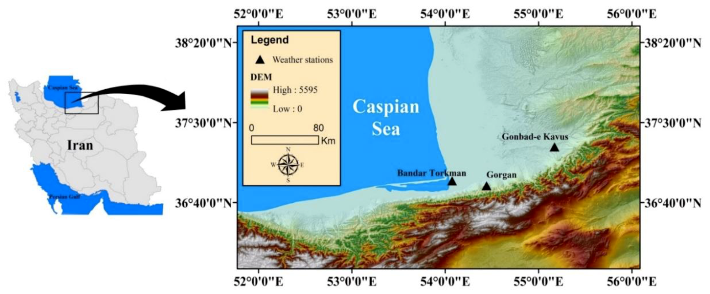
2. Study Area
3. Materials and Methods
3.1. Gaussian Process Regression (GPR)
3.2. K-Nearest-Neighbor-IBK
3.3. Random Forest (RF)
3.4. Support Vector Regression (SVR)
3.5. Model Development
3.6. Evaluation Parameters
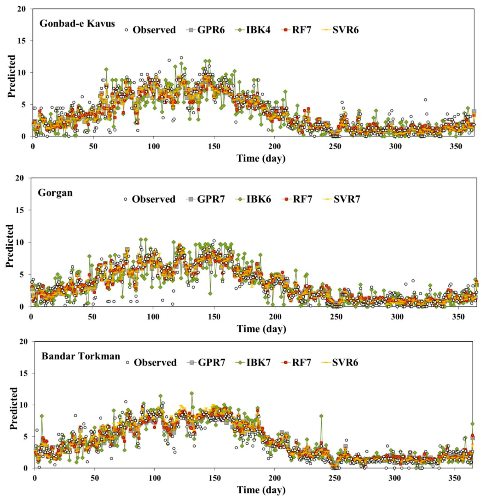
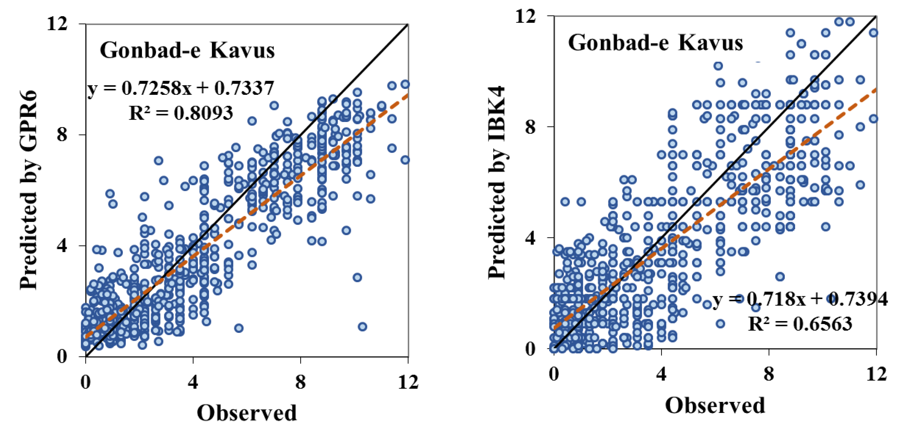
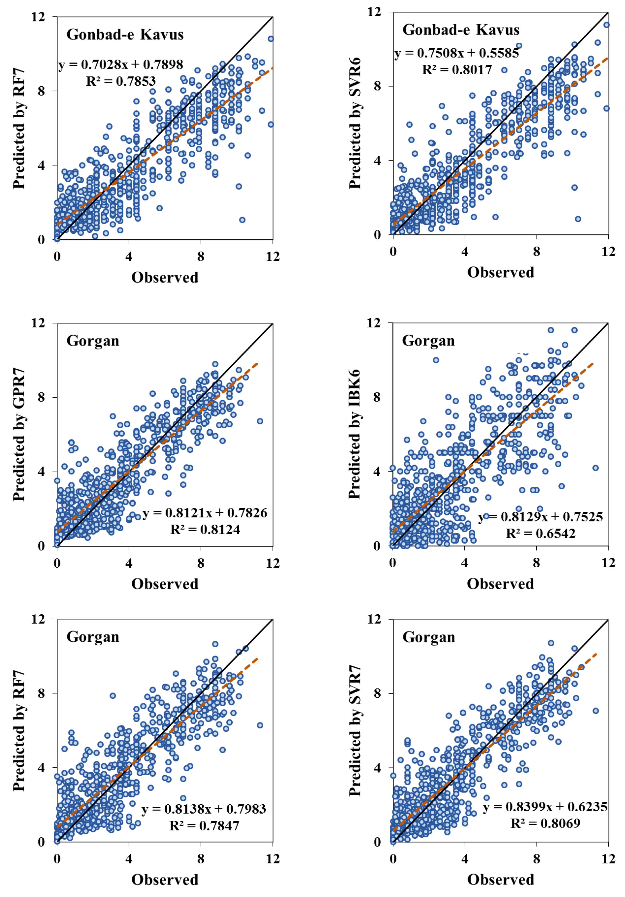
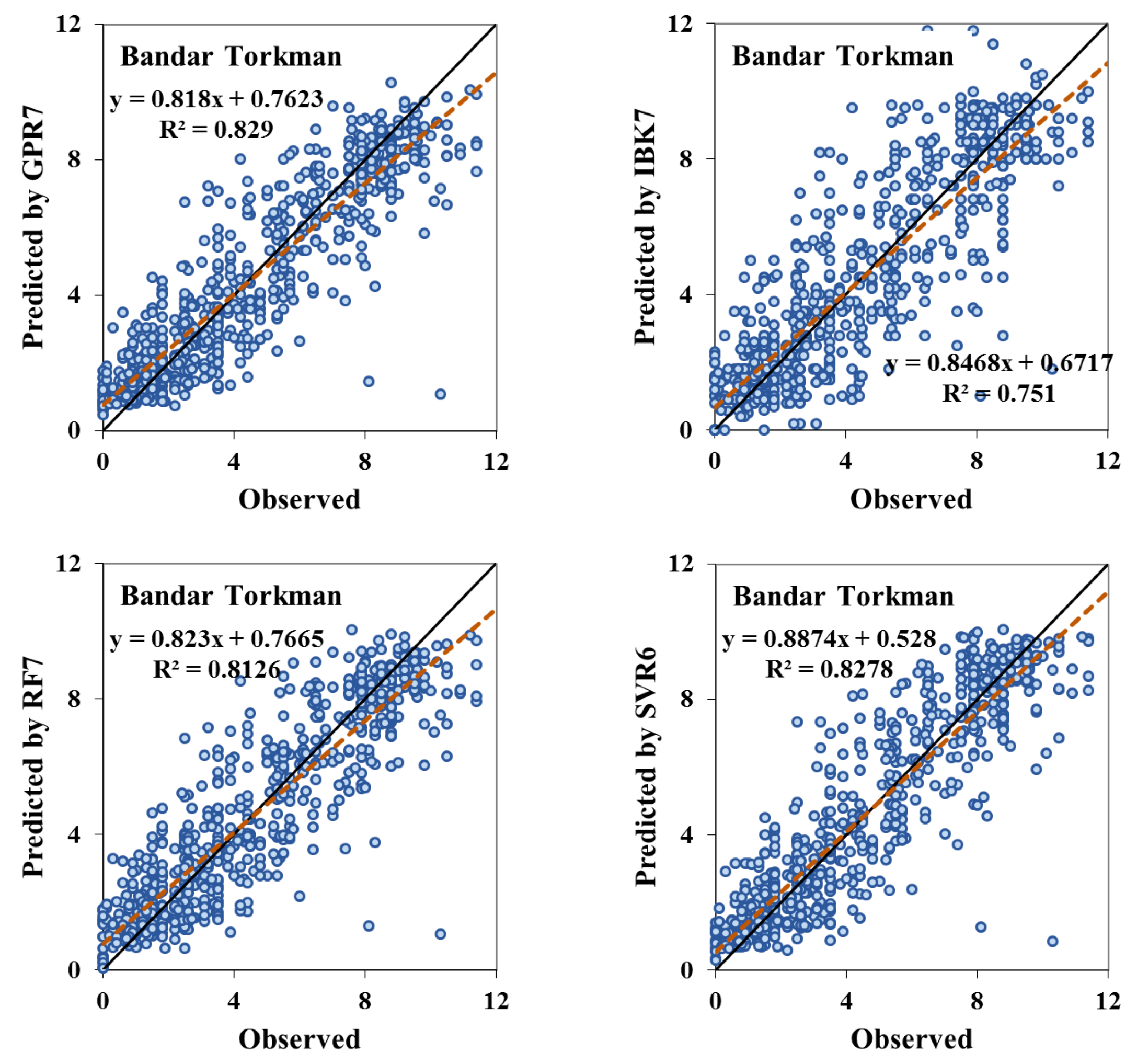
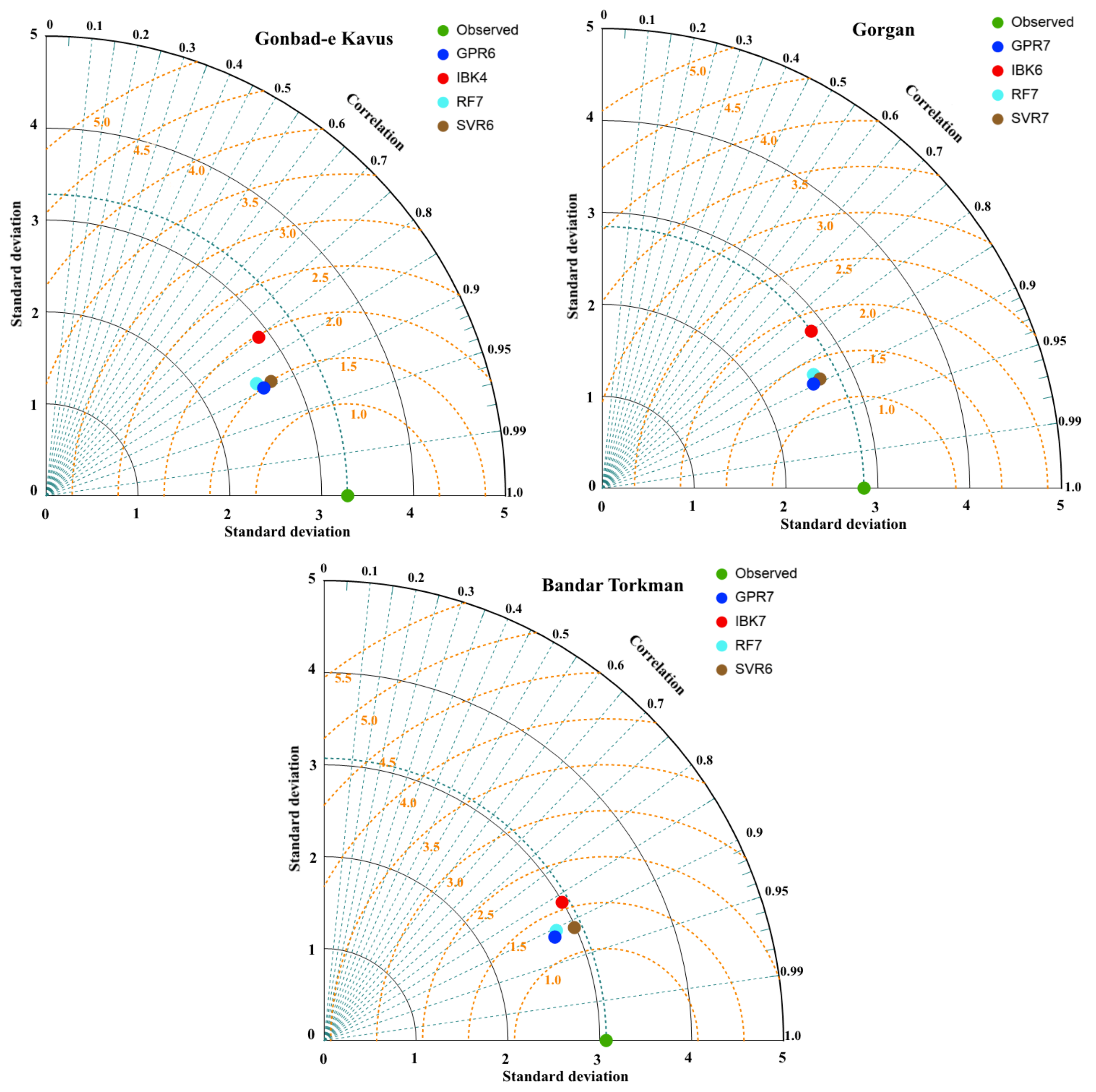
4. Results and Discussion
5. Conclusions
Author Contributions
Funding
Acknowledgments
Conflicts of Interest
References
- Yang, H.B.; Yang, D.W. Climatic factors influencing changing pan evaporation across China from 1961 to 2001. J. Hydrol. 2012, 414, 184–193. [Google Scholar] [CrossRef]
- Fan, J.; Chen, B.; Wu, L.; Zhang, F.; Lu, X.; Xiang, Y. Evaluation and development of temperature-based empirical models for estimating daily global solar radiation in humid regions. Energy 2018, 144, 903–914. [Google Scholar] [CrossRef]
- Fan, J.; Wang, X.; Wu, L.; Zhang, F.; Bai, H.; Lu, X.; Xiang, Y. New combined models for estimating daily global solar radiation based on sunshine duration in humid regions: A case study in South China. Energy Convers. Manag. 2018, 156, 618–625. [Google Scholar] [CrossRef]
- Wang, R.-Y.; Yang, X.-G.; Zhang, J.-L.; Wang, D.-M.; Liang, D.-S.; Zhang, L.-G. A Study of Soil Water and Land Surface Evaporation and Climate on Loess Plateau in the Eastern Gansu Province. Adv. Earth Sci. 2007, 22, 625. [Google Scholar]
- Monteith, J.L. Evaporation and environment. Symp. Soc. Exp. Biol. 1965, 19, 205–234. [Google Scholar] [PubMed]
- Jones, F.E. Evaporation of Water with Emphasis on Applications and Measurements; CRC Press: Boca Raton, FL, USA, 2018. [Google Scholar]
- Roderick, M.L.; Rotstayn, L.D.; Farquhar, G.D.; Hobbins, M.T. On the attribution of changing pan evaporation. Geophys. Res. Lett. 2007, 34, L17403. [Google Scholar] [CrossRef] [Green Version]
- Pereira, L.S.; Allen, R.G.; Smith, M.; Raes, D. Crop evapotranspiration estimation with FAO56: Past and future. Agric. Water Manag. 2015, 147, 4–20. [Google Scholar] [CrossRef]
- Saadi, S.; Todorovic, M.; Tanasijevic, L.; Pereira, L.S.; Pizzigalli, C.; Lionello, P. Climate change and Mediterranean agriculture: Impacts on winter wheat and tomato crop evapotranspiration, irrigation requirements and yield. Agric. Water Manag. 2015, 147, 103–115. [Google Scholar] [CrossRef]
- Smith, M.; Allen, R.; Monteith, J.; Perrier, A.; Pereira, L.; Segeren, A. Report on the Expert Consultation on Procedures for Revision of FAO Guidelines for Prediction of Crop Water Requirements; FAO: Rome, Italy, 1991. [Google Scholar]
- Abdelhadi, A.; Hata, T.; Tanakamaru, H.; Tada, A.; Tariq, M. Estimation of crop water requirements in arid region using Penman–Monteith equation with derived crop coefficients: A case study on Acala cotton in Sudan Gezira irrigated scheme. Agric. Water Manag. 2000, 45, 203–214. [Google Scholar] [CrossRef]
- Smith, M.; Allen, R.; Pereira, L. Revised FAO Methodology for Crop-Water Requirements; International Atomic Energy Agency (IAEA): Vienna, Austria, 1998. [Google Scholar]
- Wang, L.; Kisi, O.; Zounemat-Kermani, M.; Li, H. Pan evaporation modeling using six different heuristic computing methods in different climates of China. J. Hydrol. 2017, 544, 407–427. [Google Scholar] [CrossRef]
- Keskin, M.E.; Terzi, Ö. Artificial neural network models of daily pan evaporation. J. Hydrol. Eng. 2006, 11, 65–70. [Google Scholar] [CrossRef]
- Guven, A.; Kişi, Ö. Daily pan evaporation modeling using linear genetic programming technique. Irrig. Sci. 2011, 29, 135–145. [Google Scholar] [CrossRef]
- Traore, S.; Guven, A. Regional-specific numerical models of evapotranspiration using gene-expression programming interface in Sahel. Water Resour. Manag. 2012, 26, 4367–4380. [Google Scholar] [CrossRef]
- Gundalia, M.J.; Dholakia, M. Estimation of pan evaporation using mean air temperature and radiation for monsoon season in Junagadh region. Int. J. Eng. Res. Appl. 2013, 3, 64–70. [Google Scholar]
- Kisi, O.; Zounemat-Kermani, M. Comparison of two different adaptive neuro-fuzzy inference systems in modelling daily reference evapotranspiration. Water Resour. Manag. 2014, 28, 2655–2675. [Google Scholar] [CrossRef]
- Wang, L.; Kisi, O.; Hu, B.; Bilal, M.; Zounemat-Kermani, M.; Li, H. Evaporation modelling using different machine learning techniques. Int. J. Climatol. 2017, 37, 1076–1092. [Google Scholar] [CrossRef]
- Wang, L.; Niu, Z.; Kisi, O.; Li, C.A.; Yu, D. Pan evaporation modeling using four different heuristic approaches. Comput. Electron. Agric. 2017, 140, 203–213. [Google Scholar] [CrossRef]
- Malik, A.; Kumar, A.; Kisi, O. Monthly pan-evaporation estimation in Indian central Himalayas using different heuristic approaches and climate based models. Comput. Electron. Agric. 2017, 143, 302–313. [Google Scholar] [CrossRef]
- Ghorbani, M.A.; Deo, R.C.; Yaseen, Z.M.; Kashani, M.H.; Mohammadi, B. Pan evaporation prediction using a hybrid multilayer perceptron-firefly algorithm (MLP-FFA) model: Case study in North Iran. Theor. Appl. Climatol. 2018, 133, 1119–1131. [Google Scholar] [CrossRef]
- Tao, H.; Diop, L.; Bodian, A.; Djaman, K.; Ndiaye, P.M.; Yaseen, Z.M. Reference evapotranspiration prediction using hybridized fuzzy model with firefly algorithm: Regional case study in Burkina Faso. Agric. Water Manag. 2018, 208, 140–151. [Google Scholar] [CrossRef]
- Khosravi, K.; Daggupati, P.; Alami, M.T.; Awadh, S.M.; Ghareb, M.I.; Panahi, M.; Pham, B.T.; Rezaie, F.; Qi, C.; Yaseen, Z.M. Meteorological data mining and hybrid data-intelligence models for reference evaporation simulation: A case study in Iraq. Comput. Electron. Agric. 2019, 167, 105041. [Google Scholar] [CrossRef]
- Salih, S.Q.; Allawi, M.F.; Yousif, A.A.; Armanuos, A.M.; Saggi, M.K.; Ali, M.; Shahid, S.; Al-Ansari, N.; Yaseen, Z.M.; Chau, K.W. Viability of the advanced adaptive neuro-fuzzy inference system model on reservoir evaporation process simulation: Case study of Nasser Lake in Egypt. Eng. Appl. Comput. Fluid Mech. 2019, 13, 878–891. [Google Scholar] [CrossRef] [Green Version]
- Feng, Y.; Jia, Y.; Zhang, Q.; Gong, D.; Cui, N. National-scale assessment of pan evaporation models across different climatic zones of China. J. Hydrol. 2018, 564, 314–328. [Google Scholar] [CrossRef]
- Qasem, S.N.; Samadianfard, S.; Kheshtgar, S.; Jarhan, S.; Kisi, O.; Shamshirband, S.; Chau, K.-W. Modeling monthly pan evaporation using wavelet support vector regression and wavelet artificial neural networks in arid and humid climates. Eng. Appl. Comput. Fluid Mech. 2019, 13, 177–187. [Google Scholar] [CrossRef] [Green Version]
- Yaseen, Z.M.; Al-Juboori, A.M.; Beyaztas, U.; Al-Ansari, N.; Chau, K.W.; Qi, C.; Ali, M.; Salih, S.Q.; Shahid, S. Prediction of evaporation in arid and semi-arid regions: A comparative study using different machine learning models. Eng. Appl. Comput. Fluid Mech. 2020, 14, 70–89. [Google Scholar] [CrossRef] [Green Version]
- Pasolli, L.; Melgani, F.; Blanzieri, E. Gaussian process regression for estimating chlorophyll concentration in subsurface waters from remote sensing data. IEEE Geosci. Remote Sens. Lett. 2010, 7, 464–468. [Google Scholar] [CrossRef]
- Wu, X.; Kumar, V.; Quinlan, J.R.; Ghosh, J.; Yang, Q.; Motoda, H.; McLachlan, G.J.; Ng, A.; Liu, B.; Philip, S.Y. Top 10 algorithms in data mining. Knowl. Inf. Syst. 2008, 14, 1–37. [Google Scholar] [CrossRef] [Green Version]
- Hastie, T.; Tibshirani, R.; Friedman, J.; Franklin, J. The elements of statistical learning: Data mining, inference and prediction. Math. Intell. 2005, 27, 83–85. [Google Scholar]
- Breiman, L. Random forests. Mach. Learn. 2001, 45, 5–32. [Google Scholar] [CrossRef] [Green Version]
- Shi, T.; Horvath, S. Unsupervised learning with random forest predictors. J. Comput. Graph. Stat. 2006, 15, 118–138. [Google Scholar] [CrossRef]
- Boser, B.E.; Guyon, I.M.; Vapnik, V.N. A training algorithm for optimal margin classifiers. In Proceedings of the Fifth Annual Workshop on Computational Learning Theory, Association for Computing Machinery, New York, NY, USA, July 1992; pp. 144–152. [Google Scholar]
- Vapnik, V. The Nature of Statistical Learning Theory; Springer Science & Business Media: Berlin, Germany, 2013. [Google Scholar]
- Kisi, O.; Cimen, M. A wavelet-support vector machine conjunction model for monthly streamflow forecasting. J. Hydrol. 2011, 399, 132–140. [Google Scholar] [CrossRef]
- Taylor, K.E. Summarizing multiple aspects of model performance in a single diagram. J. Geophys. Res. Atmos. 2001, 106, 7183–7192. [Google Scholar] [CrossRef]
- Mosavi, A.; Ozturk, O.; Chau, K. Flood prediction using machine learning models: Literature review. Water 2018, 10, 1536. [Google Scholar] [CrossRef] [Green Version]
- Mosavi, A.; Salimi, M.; Faizollahzadeh Ardabili, S.; Rabczuk, T.; Shamshirband, S.; Varkonyi-Koczy, A.R. State of the Art of Machine Learning Models in Energy Systems, a Systematic Review. Energies 2019, 12, 1301. [Google Scholar] [CrossRef] [Green Version]
- Ouaer, H.; Hosseini, A.H.; Amar, M.N.; Seghier, M.E.A.B.; Ghriga, M.A.; Nabipour, N.; Andersen, P.Ø. Rigorous Connectionist Models to Predict Carbon Dioxide Solubility in Various Ionic Liquids. Appl. Sci. 2020, 10, 304. [Google Scholar] [CrossRef] [Green Version]
- Asadi, E.; Isazadeh, M.; Samadianfard, S.; Ramli, M.F.; Mosavi, A.; Nabipour, N.; Shamshirband, S.; Hajnal, E.; Chau, K.-W. Groundwater Quality Assessment for Sustainable Drinking and Irrigation. Sustainability 2020, 12, 177. [Google Scholar] [CrossRef] [Green Version]
- Choubin, B.; Moradi, E.; Golshan, M.; Adamowski, J.; Sajedi-Hosseini, F. An Ensemble prediction of flood susceptibility using multivariate discriminant analysis, classification and regression trees, and support vector machines. Sci. Total Environ. 2019, 651, 2087–2096. [Google Scholar] [CrossRef]
- Nabipour, N.; Mosavi, A.; Baghban, A.; Shamshirband, S.; Felde, I. Extreme Learning Machine-Based Model for Solubility Estimation of Hydrocarbon Gases in Electrolyte Solutions. Preprints 2020, 2020, 010010. [Google Scholar] [CrossRef]
- Shamshirband, S.; Hadipoor, M.; Baghban, A.; Mosavi, A.; Bukor, J.; Várkonyi-Kóczy, A.R. Developing an ANFIS-PSO Model to Predict Mercury Emissions in Combustion Flue Gases. Mathematics 2019, 7, 965. [Google Scholar] [CrossRef] [Green Version]
- Bemani, A.; Baghban, A.; Shamshirband, S.; Mosavi, A.; Csiba, P.; Varkonyi-Koczy, A.R. Applying ANN, ANFIS, and LSSVM Models for Estimation of Acid Solvent Solubility in Supercritical CO2. arXiv 2019, arXiv:1912.05612. [Google Scholar] [CrossRef]
- Riahi-Madvar, H.; Dehghani, M.; Seifi, A.; Salwana, E. Comparative analysis of soft computing techniques RBF, MLP, and ANFIS with MLR and MNLR for predicting grade-control scour hole geometry. Eng. Appl. Comput. Fluid Mech. 2019, 13, 529–550. [Google Scholar] [CrossRef] [Green Version]
- Choubin, B. Spatial hazard assessment of the PM10 using machine learning models in Barcelona, Spain. Sci. Total Environ. 2020, 701, 134474. [Google Scholar] [CrossRef] [PubMed]
- Qasem, S.N.; Samadianfard, S.; Nahand, H.S.; Mosavi, A.; Shamshirband, S.; Chau, K.W. Estimating daily dew point temperature using machine learning algorithms. Water 2019, 11, 582. [Google Scholar] [CrossRef] [Green Version]
- Samadianfard, S.; Jarhan, S.; Salwana, E.; Mosavi, A.; Shamshirband, S.; Akib, S. Support Vector Regression Integrated with Fruit Fly Optimization Algorithm for River Flow Forecasting in Lake Urmia Basin. Water 2019, 11, 1934. [Google Scholar] [CrossRef] [Green Version]
- Samadianfard, S.; Panahi, S. Estimating Daily Reference Evapotranspiration using Data Mining Methods of Support Vector Regression and M5 Model Tree. J. Watershed Manag. Res. 2019, 9, 157–167. [Google Scholar]
- Dodangeh, E.; Choubin, B.; Eigdir, A.N. Integrated machine learning methods with resampling algorithms for flood susceptibility prediction. Sci. Total Environ. 2019, 9, 135983. [Google Scholar] [CrossRef]
- Zounemat-Kermani, M.; Seo, Y.; Kim, S.; Ghorbani, M.A.; Samadianfard, S.; Naghshara, S.; Kim, N.W.; Singh, V.P. Can Decomposition Approaches Always Enhance Soft Computing Models? Predicting the Dissolved Oxygen Concentration in the St. Johns River, Florida. Appl. Sci. 2019, 9, 2534. [Google Scholar] [CrossRef] [Green Version]


| Station | Variable | Mean | Minimum | Maximum | Standard Deviation | Coefficient of Variation | Skewness | Correlation with PE |
|---|---|---|---|---|---|---|---|---|
| Gonbad-e Kavus | T (°C) | 19.2 | −6.8 | 36.8 | 8.86 | 0.46 | −0.07 | 0.85 |
| RH (%) | 66.0 | 21.5 | 98.0 | 14.16 | 0.21 | 0.03 | −0.63 | |
| W (m/s) | 1.7 | 0.0 | 7.7 | 1.07 | 0.64 | 0.72 | 0.24 | |
| S (hr) | 6.9 | 0.0 | 13.6 | 4.19 | 0.61 | −0.45 | 0.46 | |
| PE (mm/day) | 3.8 | 0.0 | 13.6 | 3.06 | 0.81 | 0.64 | 1.00 | |
| Gorgan | T (°C) | 18.4 | −4.7 | 35 | 8.42 | 0.46 | −0.08 | 0.87 |
| RH (%) | 70.2 | 20.5 | 98 | 12.22 | 0.17 | −0.06 | −0.65 | |
| W (m/s) | 2.0 | 0.0 | 10 | 1.44 | 0.71 | 0.74 | 0.28 | |
| S (hr) | 6.4 | 0.0 | 13.1 | 4.19 | 0.65 | −0.27 | 0.50 | |
| PE (mm/day) | 3.7 | 0.0 | 12.8 | 2.84 | 0.78 | 0.59 | 1.00 | |
| Bandar Torkman | T (°C) | 18.4 | −4.3 | 34.5 | 8.08 | 0.44 | −0.11 | 0.88 |
| RH (%) | 73.6 | 37.5 | 98.0 | 9.73 | 0.13 | −0.12 | −0.52 | |
| W (m/s) | 3.3 | 0.0 | 17.7 | 1.96 | 0.6 | 1.27 | 0.44 | |
| S (hr) | 6.5 | 0.0 | 13.3 | 4.12 | 0.63 | −0.33 | 0.45 | |
| PE (mm/day) | 4.4 | 0.0 | 16.0 | 3.09 | 0.71 | 0.52 | 1.00 |
| Test Type | Test Name | p-Value (Bandar Torkman) | p-Value (Gorgan) | p-Value (Gonbad-e Kavus) |
|---|---|---|---|---|
| Homogeneity Test | Pettitt’s test | <0.0001 | <0.0001 | <0.0001 |
| Buishand’s test | <0.0001 | <0.0001 | <0.0001 | |
| SNHT | <0.0001 | <0.0001 | <0.0001 | |
| VNR | <0.0001 | <0.0001 | <0.0001 | |
| Trend Test | Mann-Kendall | <0.0001 | <0.0001 | 0.599 |
| Outlier Test | Grubbs test | 0.411 | 0.60 | <0.0001 |
| Dixon test | 0.005 | 0.599 | 0.791 |
| Number | Input Parameters |
|---|---|
| 1 | T and RH |
| 2 | T and W |
| 3 | T and S |
| 4 | T, RH and W |
| 5 | T, RH and S |
| 6 | T, W, and S |
| 7 | T, RH, W and S |
| Model | Gonbad-e Kavus | Gorgan | Bandar Torkman | ||||||
|---|---|---|---|---|---|---|---|---|---|
| R | MAE (mm/day) | RMSE (mm/day) | R | MAE (mm/day) | RMSE (mm/day) | R | MAE (mm/day) | RMSE (mm/day) | |
| GPR1 | 0.898 | 1.173 | 1.575 | 0.890 | 1.014 | 1.307 | 0.894 | 1.023 | 1.372 |
| GPR2 | 0.898 | 1.170 | 1.560 | 0.884 | 1.026 | 1.337 | 0.905 | 0.973 | 1.299 |
| GPR3 | 0.894 | 1.153 | 1.550 | 0.890 | 1.001 | 1.313 | 0.900 | 1.003 | 1.346 |
| GPR4 | 0.903 | 1.148 | 1.545 | 0.897 | 0.980 | 1.265 | 0.907 | 0.972 | 1.294 |
| GPR5 | 0.900 | 1.161 | 1.561 | 0.894 | 0.993 | 1.289 | 0.898 | 1.002 | 1.344 |
| GPR6 | 0.899 | 1.128 | 1.521 | 0.897 | 0.965 | 1.265 | 0.912 | 0.939 | 1.257 |
| GPR7 | 0.904 | 1.134 | 1.530 | 0.901 | 0.958 | 1.244 | 0.912 | 0.946 | 1.254 |
| IBK1 | 0.795 | 1.547 | 2.069 | 0.784 | 1.434 | 1.895 | 0.820 | 1.375 | 1.840 |
| IBK2 | 0.784 | 1.593 | 2.106 | 0.772 | 1.40 | 1.898 | 0.823 | 1.340 | 1.817 |
| IBK3 | 0.776 | 1.585 | 2.154 | 0.788 | 1.393 | 1.865 | 0.818 | 1.391 | 1.876 |
| IBK4 | 0.810 | 1.513 | 1.991 | 0.798 | 1.4 | 1.827 | 0.833 | 1.285 | 1.737 |
| IBK5 | 0.789 | 1.543 | 2.100 | 0.804 | 1.343 | 1.824 | 0.835 | 1.291 | 1.763 |
| IBK6 | 0.809 | 1.507 | 1.994 | 0.808 | 1.340 | 1.775 | 0.844 | 1.289 | 1.745 |
| IBK7 | 0.804 | 1.521 | 2.028 | 0.799 | 1.361 | 1.841 | 0.865 | 1.179 | 1.577 |
| RF1 | 0.859 | 1.322 | 1.755 | 0.856 | 1.149 | 1.492 | 0.865 | 1.139 | 1.546 |
| RF2 | 0.844 | 1.379 | 1.814 | 0.832 | 1.186 | 1.590 | 0.876 | 1.092 | 1.484 |
| RF3 | 0.865 | 1.268 | 1.703 | 0.851 | 1.155 | 1.522 | 0.877 | 1.128 | 1.502 |
| RF4 | 0.880 | 1.239 | 1.647 | 0.875 | 1.059 | 1.387 | 0.892 | 1.023 | 1.386 |
| RF5 | 0.877 | 1.241 | 1.673 | 0.870 | 1.082 | 1.423 | 0.887 | 1.045 | 1.419 |
| RF6 | 0.879 | 1.225 | 1.621 | 0.879 | 1.030 | 1.374 | 0.900 | 1.007 | 1.349 |
| RF7 | 0.886 | 1.199 | 1.614 | 0.885 | 1.011 | 1.337 | 0.903 | 0.980 | 1.316 |
| SVR1 | 0.895 | 1.207 | 1.629 | 0.888 | 1.006 | 1.317 | 0.891 | 1.018 | 1.389 |
| SVR2 | 0.896 | 1.184 | 1.585 | 0.883 | 1.017 | 1.340 | 0.904 | 0.971 | 1.314 |
| SVR3 | 0.892 | 1.154 | 1.574 | 0.889 | 0.984 | 1.315 | 0.9 | 1.003 | 1.358 |
| SVR4 | 0.901 | 1.178 | 1.590 | 0.893 | 0.982 | 1.284 | 0.906 | 0.961 | 1.298 |
| SVR5 | 0.894 | 1.186 | 1.619 | 0.894 | 0.974 | 1.287 | 0.895 | 1.009 | 1.368 |
| SVR6 | 0.895 | 1.129 | 1.550 | 0.895 | 0.962 | 1.278 | 0.911 | 0.943 | 1.275 |
| SVR7 | 0.898 | 1.146 | 1.572 | 0.898 | 0.958 | 1.262 | 0.909 | 0.960 | 1.278 |
© 2020 by the authors. Licensee MDPI, Basel, Switzerland. This article is an open access article distributed under the terms and conditions of the Creative Commons Attribution (CC BY) license (http://creativecommons.org/licenses/by/4.0/).
Share and Cite
Shabani, S.; Samadianfard, S.; Sattari, M.T.; Mosavi, A.; Shamshirband, S.; Kmet, T.; Várkonyi-Kóczy, A.R. Modeling Pan Evaporation Using Gaussian Process Regression K-Nearest Neighbors Random Forest and Support Vector Machines; Comparative Analysis. Atmosphere 2020, 11, 66. https://doi.org/10.3390/atmos11010066
Shabani S, Samadianfard S, Sattari MT, Mosavi A, Shamshirband S, Kmet T, Várkonyi-Kóczy AR. Modeling Pan Evaporation Using Gaussian Process Regression K-Nearest Neighbors Random Forest and Support Vector Machines; Comparative Analysis. Atmosphere. 2020; 11(1):66. https://doi.org/10.3390/atmos11010066
Chicago/Turabian StyleShabani, Sevda, Saeed Samadianfard, Mohammad Taghi Sattari, Amir Mosavi, Shahaboddin Shamshirband, Tibor Kmet, and Annamária R. Várkonyi-Kóczy. 2020. "Modeling Pan Evaporation Using Gaussian Process Regression K-Nearest Neighbors Random Forest and Support Vector Machines; Comparative Analysis" Atmosphere 11, no. 1: 66. https://doi.org/10.3390/atmos11010066