

Abstract
During the flapping motion of a fish's tail, the caudal fin exhibits antero-posterior bending and dorso-ventral bending, the latter of which is referred to as chord-wise bending herein. The impact of chord-wise tip curvature on the hydrodynamic forces for flapping plates is investigated to explore potential mechanisms to improve the maneuverability or the performance of autonomous underwater vehicles. First, actuated chord-wise tip curvature is explored. Comparison of rigid curved geometries to a rigid flat plate as a baseline suggests that an increased curvature decreases the generated forces. An actuated plate with a dynamic tip curvature is created to illustrate a modulation of this decrease in forces. Second, the impact of curvature is isolated using curved plates with an identical planform area. Comparison of rigid curved geometries as a baseline corroborates the result that an increased curvature decreases the generated forces, with the exception that presenting a concave geometry into the flow increases the thrust and the efficiency. A passively-actuated plate is designed to capitalize on this effect by presenting a concave geometry into the flow throughout the cycle. The dynamically and passively actuated plates show potential to improve the maneuverability and the efficiency of autonomous underwater vehicles, respectively.
Export citation and abstract BibTeX RIS
1. Introduction
In recent decades, the development of underwater vehicles for deep sea exploration, search and recovery, equipment inspection and repair, and military operations has rapidly increased. Manned underwater vehicles [1] are being replaced by remotely operated vehicles (ROVs) [2] due to their increased safety, reduced deployment costs, and extended mission durations. However, ROVs are controlled by humans, which limits their mission duration due to operator fatigue. Futhermore, communication with the vehicle requires either a long tether, which has a maximum practical length, or radio waves, which introduce a significant latency due to their travel time in water. These limitations have motivated the development of autonomous underwater vehicles (AUVs) to eliminate operator fatigue and the necessity of a tether. As technology continues to advance, new designs [3] and control mechanisms [4] are developed, further increasing the potential for faster, more maneuverable, and more efficient AUVs. Inspiration for novel designs has recently come from nature [5], primarily based on the flapping motion used by fish, which have evolved to develop fast, efficient, and maneuverable locomotion.
The flapping motion used by fish is commonly studied by either simplifying or mimicking the motion. For simplification, the flapping motion is often approximated as a plate pitching [6], heaving [7], or pitching and heaving simultaneously [8]. For pitching plates, work has been conducted to investigate the effect of the plate's kinematics and the flexibility on the wake and the generated forces. Schnipper et al [9] mapped the phase diagram of the vortex street behind a symmetric airfoil as a function of the stroke angle and the Strouhal number  . Here, f is the frequency of oscillation, t is the maximum thickness of the airfoil, and
  is the freestream velocity. Kim and Gharib [10] used defocused digital particle image velocimetry (DDPIV) [11], a quantitative 3D flow visualization technique, to examine the vortex structures formed behind pitching flat plates during their initial stroke. They found that the flow rolls up on the suction side of the plate forming a horseshoe-shaped vortex composed of two edge vortices connected by a tip vortex. This vortex structure remains attached and follows the trajectory of the plate with minimal outwards motion from the plate. Furthermore, their investigation highlighted the importance of spanwise flow in the generation of tip vortices and thrust. Dai et al [12] showed that flexible plates with a reduced stiffness
  of 5 have the greatest propulsive efficiency; reduced stiffness can be thought of as a ratio of a material's bending resistance to the bending moment applied by the fluid. Here, E is the elastic modulus, I = ct3/12 is the second moment of area, c is the chord length, t is the thickness, s is the span, and ρ is the density of the fluid. Lu et al [13] studied large amplitude motions and found that increasing either the amplitude or the reduced frequency
  generates a greater thrust and requires more power, but simultaneously increasing both the amplitude and the reduced frequency decreases the propulsive efficiency. These works have highlighted the importance of stroke angle, frequency, and flexibility.
Advances in technology and materials have enabled more accurate mimicry of the flapping motion used by fish. A few examples in robotics utilize an assembly of strings and pulleys [14], macro fibre composites [15], ionic polymer-metal composites [16], or shape memory alloys [17] to mimic the antero-posterior bending of the caudal fin. A review of the commonly used actuation mechanisms was conducted by Karpelson et al [18]. By contrast, the dorso-ventral bending of the caudal fin, documented by Bainbridge [19], remains largely unexplored to the best of the authors' knowledge. In his study, dorso-ventral bending (referred to as chord-wise bending herein), where the two tips of the caudal fin bend towards each other on a dace (Leuciscus leuciscus) was proposed to help smooth out the intermittent thrust generated by the tail and assist in braking; a concave caudal fin geometry was presented towards the incoming fluid when attempting a quick-stop maneuver. The maximum tip radius of curvature achieved by the dace was approximately 55 mm with a tip curvature aspect ratio  of approximately 0.22; here, h and
  are the height and width of the curved geometry (figure 1(c)). Studies of bluegill sunfish (Lepomis macrochirus) [20], which predominately maneuver using their pectoral fins, documented a cupping motion of the pectoral fins when swimming, creating a bent geometry similar to the dorso-ventral bending of the dace's caudal fin. This motion was recreated using actuated fin rays, which behave similarly to a bimetallic strip, and was shown to significantly reduce drag [21].
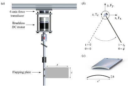
Figure 1. (a) Side view of the experimental setup and the definition of the span s and the chord c. (b) Definition of the stroke angle ϕ, the stroke time ts, and the positive direction of the x, y, and z axes, the forces Fx and Fy, and the torque Tz. The dashed line denotes the original position of the plate at the beginning of the first half of the cycle. The curved arrow denotes the direction of motion during the first half of the cycle; during the second half of the cycle, the motion is reversed. (c) Definition of the height h and the width  measured at the tip of the test plates.
Download figure:
Standard image High-resolution imageThe purpose of this study is to investigate the effects of chord-wise tip curvature on the forces and torques generated by flapping plates as a simplified model of the dorso-ventral bending of a fish's caudal fin during locomotion. Here, the flapping motion of a fish's caudal fin during locomotion is approximated by the pitching motion of plates. This motion is used to emulate thunniform swimming where the caudal fin is the primary source of thrust and lateral motion [22]. The plates are compared at different stroke angles ϕ and stroke times ts (figure 1(b)) to assess their performance using the experimental setup described in section 2. First, the concept of emulating active chord-wise bending, similar to the dorso-ventral bending seen in the caudal fin, is explored. A baseline is established by comparing a rigid flat plate with rigid curved plates in section 3.1. This is followed by the implementation of a dynamically-actuated design in section 3.2. Second, the impact of curvature is isolated using plates with the same planform area. This is in contrast to the previous cases which emulate physically curving the plates which reduces the plate's planform area. Similar to the previous case, a baseline is established using rigid curved plates in section 3.3, followed by a brief discussion on the impact of the planform area in section 3.4 and the implementation of a passively-actuated plate in section 3.5. Finally, the generated wake behind select test plates are investigated in section 3.6 to explain their performance. A summary of the results is presented in section 3.7. All tests begin from quiescent flow and continue without an imposed co-flow to investigate the infinite Strouhal number limit.
2. Experimental setup
The setup shown in figure 1(a) pitches the test plates, shown with their acronyms, in figure 2. The first letter of 'R' or 'A' denotes a rigid (R) static plate or an actuated (A) plate, respectively. The second letter of 'C' corresponds to plates which emulate physically curving (C) the two free corners of a plate towards each other and therefore have a reduced planform area. The second letter of 'M' corresponds to plates used to isolate the impact of tip curvature and therefore have the same chord, the same span, and a matched (M) planform area, 5470 mm2, as those of the baseline rigid flat plate. The numbers '0', '1', and '2' are used to qualitatively distinguish between no, small, and large tip curvatures. The addition of '-F' to the acronym indicates that a fence (F) is added to the tip of the plate.
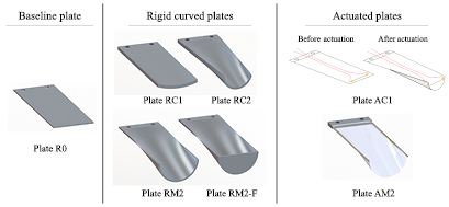
Figure 2. Render of the test plates used. 'R' denotes a rigid static plate, 'A' denotes an actuated plate, 'C' denotes a plate emulating physically curving the two free corners towards each other reducing the planform area, 'M' denotes a plate with a matched planform area to that of the baseline flat plate, and '-F' indicates that a fence is added to the tip of the plate. The numbers '0', '1', and '2' qualitatively distinguish between no, small, and large tip curvatures.
Download figure:
Standard image High-resolution imageA full cycle consists of two strokes. The forward and the backward strokes are defined as the first and the second stroke in a cycle, respectively. It should be noted that the rigid curved plates present a concave geometry towards the incoming flow during the forward stroke and a convex geometry towards the incoming flow during the backward stroke. All of the test plates are compared with the baseline aluminum rigid flat plate  with a span s = 110.5 mm, a chord length c = 50 mm, a thickness t = 1.65 mm, a planform area A = 5520 mm2, and an aspect ratio s/c = 2.21; all other plates have the same span and chord unless specified otherwise.
Plates  and
and  are rapidly-prototyped 4 mm thick plastic plates with a tip chord-wise radius of curvature of 72.0 mm and 15.9 mm, tip curvature aspect ratio
  of 0.0878 and 0.5 (figure 1(c)), and a planform area of 5410 mm2 and 4700 mm2, respectively. The chords of plates
  and
and  decrease linearly from 50 mm at the root to 49 mm and 31.8 mm, respectively, at the tip of the plate. Plate
  is a dynamically-actuated plate with a controllable tip curvature realized by attaching a 35 mm long 0.254 mm diameter Dynalloy, Inc. Flexinol actuator wire made of Nitinol, a shape memory alloy that contracts when heated to 70 °C by an electric current, to the tip of a 0.381 mm and a 0.508 mm thick polycarbonate plate. Stronger material or thicker polycarbonate plates exceed the actuation capability of the Nitinol wire. These plates have a reduced stiffness
  of 1.094 and 1.459, respectively. The 0.381 mm thick plate is tested at
  ° in ts = 2 s while the 0.508 mm thick plate is tested at
  ° in ts = 1 s (figure 1(b)). For
  , the bending moment applied by the fluid is comparable to the material's resistance to bending, meaning the plate significantly deforms throughout the cycle. This definition of K is similar to that used by Dai et al [12], except here,
  is the average speed of the trailing edge. The Nitinol wire, selected due to its large deflection and actuation force compared with other mechanisms [18], has a maximum strain rate and pulling force of 4.5% and 8.74 N, respectively. Actuation occurs through a BOP 50-4M controllable power supply, with a voltage range of ±50 V and a current range of ±4 A, using signals from a National Instruments USB-6211 DAQ. When actuated in 20 °C water using a 0-4 A square wave, the tip obtains a maximum radius of curvature of 43 mm and a
  in 0.05 s. The relaxation time of the wire is approximately 0.5 s; however, during the pitching motion, the relaxation time decreases due to convection cooling.
Plates  and
and  are rapidly-prototyped, 2 mm thick plastic plates with a tip chord-wise radius of curvature of 23 mm and a
  . The plates are identical except that plate
  has a 2 mm thick fence attached to the tip. Plate
  is a passively-actuated plate that snap-buckles into a inextensible curved geometry similar to that of plate
  following a change in direction. This is accomplished by attaching a 0.02 mm thick polycarbonate sheet, with a pre-curved 23 mm tip radius of curvature to a 1.59 mm diameter brass wire frame. The radius of curvature is identical to that of plates
  and
and  . It should be noted that plate
  presents a concave geometry into the flow during both the forward and the backward strokes and that polycarbonate is effectively inextensible under the tested flow conditions, meaning the material does not stretch during the motion. A summary of the test plates and their acronyms is shown in table 1.
Table 1. Abbreviations and characteristics of the plates.
| Plate | Type | A(mm2) | β(—) | Note |
|---|---|---|---|---|
 |
Rigid | 5520 | 0 | — |
 |
Rigid | 5410 | 0.0878 | — |
 |
Rigid | 4700 | 0.5 | — |
 |
Rigid | 5470 | 0.5 | — |
 |
Rigid | 5470 | 0.5 | Fence |
 |
Actuated | 5520 | 0.13 | Nitinol |
 |
Actuated | 5520 | 0.5 | Snap-buckle |
The plates are pitched by a Maxon EC 45 flat DC brushless motor, to which a 4.3:1 reduction gearhead and a 2048 counts per turn encoder are attached. The motor is controlled using an EPOS2 24/5 digital position controller and driven with a sinusoidal velocity profile generated from a National Instruments USB-6211 DAQ board. The stroke angles ϕ studied are 45°, 60°, 75°, and 90°, while the stroke times ts studied are 2, 1, 0.75, and 0.5 s for a single stroke (figure 1(b)). These kinematics give a range of Reynolds numbers  , used to characterize the flow conditions from a ratio of inertial to viscous forces, between 7920 and 19 000 based on the average tip velocity of the plate
  , the average angular velocity of the plate
  , the span of the plate s, and the kinematic viscosity of the fluid ν. It should be noted that the rigid plates do not exhibit any significant deformation during any of the trials. The performance of the plates is evaluated by investigating the instantaneous and the average forces and torques generated per cycle after reaching steady state; the average values per cycle are typically calculated from five trials, with at least eight cycles per trial. The forces and torques used to assess the performance of each plate are measured using an ATI Nano 43, a 6-axis force and torque transducer, with a maximum capacity of 18 N and 250 N · mm and a resolution of 0.0039 N and 0.050 N · mm. The average side force, thrust, and torque coefficients are written as:
The instantaneous versions of these coefficients are identical but do not use averaged quantities denoted by an overline. The signs and directions of the forces and torques are consistent with the coordinate system illustrated in figure 1(b). The efficiency is defined in two ways:
Here,  compares the thrust to the side force, typically used in biology, while
  compares the thrust generated to the required torque, similar to a mechanical efficiency. It should be noted that Tz can be interpreted as an alternative description for side force, as Tz is related to the force normal to the plate at all times throughout the motion. The error bars shown for
  ,
,  ,
,  , and
, and  in section 3 are computed from the standard deviation of the mean CS, CT, and
  per cycle and although they are only plotted in one direction, they are symmetric. All experiments are conducted in a 0.762 m long, 0.305 m wide, and 0.483 m tall water tank starting from quiescent flow. As the tank is small compared with the size of the plates, only 10 cycles are recorded to minimize re-circulation effects. To minimize free surface effects, the plates are fully submerged.
The generated flow field is investigated qualitatively through dye visualization [23] during the first forward stroke and quantitatively through digital particle image velocimetry (DPIV) [24] once the flow has reached steady state. Dye visualization is conducted by injecting red food coloring at 500 μl min−1 from two Harvard Apparatus dual syringe pumps through four separate internal chambers in rapidly prototyped 3.81 mm thick PLA plastic versions of the test plates. The locations of the dye injection points are dimensioned in figure 3. These locations were selected through a trial-and-error processes to best visualize the flow and are identical for all of the dye injection test plates. Images of the generated flow field were captured in color using a Canon Vixia HF R700 camcorder at 60 frames per second angled normal to the initial position of the plate to provide a better view of the developing vortex structures. DPIV is realized by first seeding the flow with Potters Industries silver-coated hollow glass spheres (mean density 1.60 g · cc−1 and diameter 13 μm). Then, illuminating the near wake using an Opto Engine LLC 3W continuous laser to create a laser sheet along the mid-plane of the pitching plates; the mid-plane is the same as the line of symmetry denoted by the dashed line in figure 3. Finally, recording the position of the illuminated particles, which follow the flow, with an IDT Motion Pro Y7 at 500 frames per second. By recording the position of the particles in time at a known frame rate, quantitative information about the flow field can be obtained.
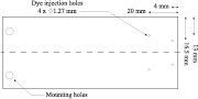
Figure 3. Location of the dye injection points relative to a corner of the tip. The dye injection points are identical for all of the dye injection plates. All dye injection holes have the same diameter. The mid-plane, or line of symmetry, for the plate is indicated by the dashed line.
Download figure:
Standard image High-resolution image3. Results and discussion
3.1. Rigid curved plates as a baseline
The two rigid curved plates with a small and a large tip radius of curvature, plates  and
and  , respectively, are compared with a rigid flat plate, plate
  . This comparison is made to establish a baseline regarding the effect of curvature on the generated forces and torques if a rigid flat plate could be actuated into a similar curved geometry. The curvature of plate
  is selected to be similar to the maximum achievable curvature through dynamic actuation with plate
  , while the curvature of plate
  is selected as a semicircle to investigate the impact of curvatures larger than plate
  can realize. The instantaneous CS, CT, and
  as functions of the non-dimensional time
  are shown in figure 4 for a typical cycle and the
  ,
,  ,
,  , and
, and  per cycle are shown in figure 5 for plates
  ,
,  , and
, and  . The forward stroke, when a concave geometry is presented by the rigid curved plates towards the incoming flow, corresponds to 0 < t* < 0.5 while the backward stroke, when a convex geometry is presented towards the incoming flow, corresponds to 0.5 < t* < 1.
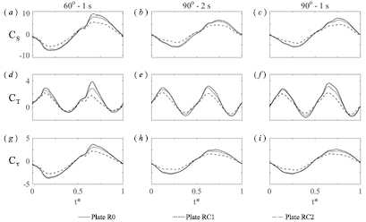
Figure 4. Typical instantaneous CS (a)–(c), CT (d)–(f), and  (g)–(i) as functions of t* over one full cycle after reaching steady state for plates
  ,
,  , and
, and  . Panels ((a), (d), (g)), ((b), (e), (h)), and ((c), (f), (i)) have the same kinematics given in the form
  . The first half of all of the plots, 0 < t* < 0.5, corresponds to the forward stroke, when the rigid curved plates are concave to the incoming flow, while the second half of all of the plots, 0.5 < t* < 1, corresponds to the backward stroke, when the rigid curved plates are convex to the flow.
Download figure:
Standard image High-resolution image
Figure 5. Average side force coefficient  (a), average thrust coefficient
  (c), and two definitions of efficiency,
  (b) and
  (d), over a cycle as functions of the plate kinematics for plates
  ,
,  , and
, and  . The x-axis indicates the stroke angle ϕ on the top row and the stroke time ts on the bottom row.
Download figure:
Standard image High-resolution imageComparison of the instantaneous CS in figures 4(a)–(c) between the three plates for all sets of kinematics shows that increasing the curvature decreases the peak side force generated, even when accounting for the difference in the planform area with the denominator of CS. From the data shown in figure 4, plates  and
and  decrease the peak side force by 5.3% and 30.8% on average during the forward stroke, respectively, and by 10.8% and 38.3% on average during the backward stroke, respectively, when compared with plate
  . The results from the instantaneous
  in figures 4(g)–(i) corroborates the results from CS. Comparison of the instantaneous CT in figures 4(d)–(f) between the three plates for all sets of kinematics shows a decrease in the peak thrust generated by plates
  and
and  compared to
  . The data shown in figure 4 indicates that plates
  and
and  decrease the peak thrust by 9.8% and 25.9% on average during the forward stroke, respectively, and by 15.2% and 43.3% on average during the backward stroke, respectively, when compared with plate
  . These results can be attributed to the reduced planform area of plates
  and
and  creating a more streamlined geometry further discussed in section 3.4. A more streamlined body opposes the flow less, decreasing the side force, and pushes less fluid in the thrust direction, decreasing the generated thrust. Regarding the difference between the forward and the backward strokes, the greater decrease in side force is due to the lower drag coefficient of a convex geometry compared with a concave geometry [25], while the greater decrease in thrust is due to a convex geometry creating a significant amount of suction, highlighted in section 3.6.
Comparison of  and
and  between the three plates in figures 5(a) and (c), respectively, corroborates the previous conclusion from the instantaneous CS and CT that an increased curvature decreases all of the generated forces. It should be noted that because plates
  and
and  present a different geometry towards the incoming flow during the forward and the backward strokes, a net side force is generated. The net side force is computed as
  in contrast to the average side force computed as
  in
in  . The net side forces generated by plates
  and
and  are 4.0% and 7.3% of the average side force generated by plate
  , respectively, in the direction opposite that of the forward stroke. This would cause an AUV to turn if a static geometry is used as a propulsor. A reduction in all of the forces could increase the efficiency if the side force or the torque is reduced more than the thrust. However, as shown in figures 5(b) and (d), both measures of efficiency for plates
  and
and  do not differ significantly from those for plate
  .
.
3.2. Dynamic chord-wise tip curvature actuation
The Nitinol-actuated plate  is used to determine the impact of a dynamically-actuated curvature. The actuation profiles used to contract the Nitinol wire are created by modifying the duty cycles of square waves with an identical frequency to that of the motion. Actuation profiles 1, 2, and 3 have duty cycles (DC) of 12.5%,
  , and
, and  , respectively, with phase angles
  of 67.5°, 0°, and 0°, respectively, for actuation during the forward stroke and phase angles
  of 247.5°, 180°, and 180°, respectively, for actuation during the backward stroke. These actuation profiles cause the wire to actuate and remained contracted during the forward stroke from a t* of 0.1875 to 0.3125, 0 to 0.25, and 0 to 0.5 respectively and during the backward stroke from a t* of 0.6875 to 0.8125, 0.5 to 0.75, and 0.5 to 1 respectively. Characteristics of the actuation profiles and the t* intervals when the plates are contracted are summarized in tables 2 and 3. The parameters were selected to cover a variety of possible profiles to assess whether the decrease in forces could be triggered and maintained effectively and arbitrarily. It should be noted that within a single trial, actuation only occurs during either the forward or the backward stroke.
Table 2. Characteristics of the actuation profiles.
| Profile | DC ( ) ) |
  |
  |
|---|---|---|---|
| 1 | 12.5 | 67.5 | 247.5 |
| 2 | 25 | 0 | 180 |
| 3 | 50 | 0 | 180 |
Table 3. Contraction timing of the actuation profiles.
| Profile | Contracted duration (t*) | |
|---|---|---|
| During forward stroke | During backward stroke | |
| 1 | 0.1875–0.3125 | 0.6875–0.8125 |
| 2 | 0–0.25 | 0.5–0.75 |
| 3 | 0–0.5 | 0.5–1.0 |
The impact of actuation is assessed by evaluating the difference in the generated forces between actuated and unactuated cases. These instantaneous differences in CS and CT are denoted  and
and  , respectively, in figure 6 for a typical cycle. The dotted horizontal lines in figure 6 correspond to the noise level of the transducer during the motion, computed from the maximum
  and
and  , between trials with identical kinematics when no actuation occurs. The solid line corresponds to actuation during the forward stroke, while the dashed line corresponds to actuation during the backward stroke. For a 60° stroke angle and a 1 s stroke time, convection cooling during the forward stroke, when the incoming water flows directly over the wire, prevents actuation. It should be noted that the solid horizontal line at zero is only meant to highlight the zero-line and does not correspond to any data. The results for the 0.381 mm thick polycarbonate plate with a 90° stroke angle and a 2 s stroke time using actuation profiles 1 and 2 are shown in figures 6(a)–(d), while the results for the 0.508 mm thick polycarbonate plate with a 60° stroke angle and a 1 s stroke time using actuation profiles 1 and 3 are shown in figures 6(e)–(h).
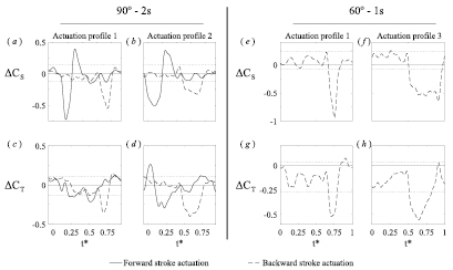
Figure 6. Typical instantaneous  ((a), (b), (e), (f)) and
  ((c), (d), (g), (h)) as functions of t* over one full cycle after reaching steady state for plate
  . Panels (a)–(d) correspond to the 0.381 mm thick polycarbonate plate with a 90° stroke angle and a 2 s stroke time, while panels (e)–(h) correspond to the 0.508 mm thick polycarbonate plate with a 60° stroke angle and a 1 s stroke time. Panels ((a), (c)), ((b), (d)), ((e), (g)), and ((f), (h)) use the actuation profiles indicated on the top of panels ((a), (b), (e), (f)). The characteristics of the actuation profiles and the t* intervals when the plates are contracted are summarized in tables 2 and 3.
Download figure:
Standard image High-resolution imageComparison of  or
or  in figure 6 across all actuation profiles shows that the forces are decreased whenever the plate is actuated, which corroborates the previous conclusion regarding the impact of curvature, with the added benefit that the reduction in forces can be triggered and maintained arbitrarily. This can be seen by comparing the duration of the decrease in forces between actuation profiles 1 and 3 in figures 6(e)–(h). Using actuation profile 1, the largest impact is achieved; the maximum reduction in CS is by 12.8% and 9.0% while that in CT is by 8.8% and 12.3% at a 90° stroke angle with a 2 s stroke time and a 60° stroke angle with a 1 s stroke time, respectively, when compared to the case without actuation. It should be noted that characterization of the Nitinol wire by actuating the wire on a motionless plate in quiescent fluid generates forces below the noise threshold. This implies that the decrease in forces is primarily due to a static change in curvature rather than a dynamic bending motion. These results show that dynamic chord-wise curvature control through Nitinol wire actuation can be triggered and maintained effectively to reduce the generated forces by approximately
  . Furthermore, this decrease in the forces is comparable to the decrease in the peak amplitude of CS and CT from plate
  , which had a similar chord-wise tip radius of curvature and β as plate
  , meaning that if greater curvatures could be realized, the forces could potentially be decreased by approximately
  , as seen with plate
  . Characterization of the influence of flexibility will require future studies.
3.3. Isolating the effect of curvature with rigid baselines
Plate  is used to isolate the effect of curvature as the only difference between plates
  and
and  is that plate
  has a tip radius of curvature of 23 mm and a β of 0.5. Plate
  is used to study the impact of spanwise flow, which has been shown to significantly affect the generation of tip vortices and thrust [10]. By attaching a fence to the tip of plate
  to create plate
  , flow in the spanwise direction near the tip of the plate is impaired because here, during the forward stroke, the flow is redirected normal to the plate. The instantaneous CS, CT, and
  as functions of t* are shown in figure 7 for a typical cycle and the
  ,
,  ,
,  , and
, and  per cycle are shown in figure 8 for plates
  ,
,  , and
, and  .
.
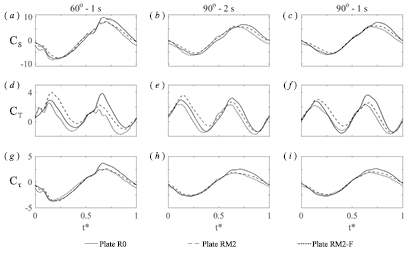
Figure 7. Typical instantaneous CS (a)–(c), CT (d)–(f), and  (g)–(i) as functions of t* over one full cycle after reaching steady state for plates
  ,
,  , and
, and  . Panels ((a), (d), (g)), ((b), (e), (h)), and ((c), (f), (i)) have the same kinematics given in the form
  . The first half of all of the plots, 0 < t* < 0.5, corresponds to the forward stroke, when the rigid curved plates are concave to the incoming flow, while the second half of all of the plots, 0.5 < t* < 1, corresponds to the backward stroke, when the rigid curved plates are convex to the incoming flow.
Download figure:
Standard image High-resolution image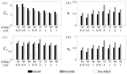
Figure 8. Average side force coefficient  (a), average thrust coefficient
  (c), and two definitions of efficiency,
  (b) and
  (d), over a cycle as functions of the plate kinematics for plates
  ,
,  , and
, and  . The x-axis indicates the stroke angle ϕ on the top row and the stroke time ts on the bottom row.
Download figure:
Standard image High-resolution imageComparison of the instantaneous CS in figures 7(a)–(c) between plates  and
and  shows that curvature decreases the peak side force generated, similar to the conclusion from section 3.1. However, adding a fence with plate
  causes the side force generated during the accelerating portion of the forward stroke to approach that generated by the baseline flat plate. The results from the instantaneous
  in figures 7(g)–(i) corroborate the results from CS. Comparison of the instantaneous CT in figures 7(d)–(f) between the plates
  and
and  shows that curvature significantly decreases the thrust generated during the backward stroke, similar to the previous conclusion from section 3.1, but, interestingly, increases the thrust generated during the forward stroke; using the data in figure 7, plate
  increases the peak thrust generated by 22.4% on average during the forward stroke but decreases the peak thrust by 26.4% on average during the backward stroke compared to plate
  . However, the addition of a fence with plate
  negates the benefit of presenting a concave geometry into the flow, causing the thrust during the forward stroke to decrease even below that of the rigid flat plate.
Comparison of the overall forces generated and the efficiency per cycle in figure 8 corroborate the previous result that plate  decreases the side force generated and increases the thrust generated, which may not be evident as plate
  increases the thrust during the forward stroke but decreases the thrust during the backward stroke. Furthermore, the addition of a fence decreases the performance of plate
  . As expected, because plate
  decreases the side force and increases the thrust, the efficiencies
  and
and  are increased by 34.3% and 36.4%, respectively. Additionally, the net side force generated is only 3.3% of the average side force of the baseline flat plate, meaning that replacing a flat plate propulsor with a curved plate of an identical planform area may be viable.
3.4. Brief discussion of planform area
The impact of the planform area can be isolated by comparing the results from plates  and
and  because they have an identical β but different planform areas. Comparison of the instantaneous CS between the two plates in figures 4(a)–(c) and 7(a)–(c), respectively, shows that curvature alone (comparing plate
  to
to  ) has a minimal effect during the forward stroke and a small effect during the backward stroke. Therefore, the result that plate
  decreases the peak CS and the overall
  per cycle more than plate
  decreases those when both are compared against plate
  must be accounted for by plate
  's reduced planform area (due to its smaller chord near the tip of the plate). This provides further evidence that decreasing the planform area creates a more streamlined geometry which reduces the side force, previously suggested in section 3.1.
Comparison of the instantaneous CT between plates  and
and  in figures 4(d)–(f) and 7(d)–(f), respectively, shows that the benefit of presenting a concave geometry towards the incoming flow is negated if the planform area is reduced. These results show that modifying the planform area by changing the chord near the tip of the plate can either significantly increase or decrease the generated thrust during the forward stroke. Furthermore, this highlights the required interaction between the planform area and the curvature to increase the thrust generated during the forward stroke which is illustrated in section 3.6.
3.5. Passive chord-wise tip curvature actuation
Motivated by the results from plate  , plate
  is designed to passively snap-buckle and present a concave geometry into the flow during both the forward and the backward strokes. The instantaneous CS, CT, and
  as functions of t* are shown in figure 9 for a typical cycle and the
  ,
,  ,
,  , and
, and  per cycle are shown in figure 10 for plates
  ,
,  , and
, and  . Plate
  is tested on a smaller subset of the kinematics as only large angular velocities induce snap-buckling.
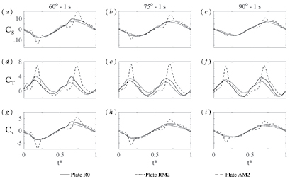
Figure 9. Typical instantaneous CS (a)–(c), CT (d)–(f), and  (g)–(i) as functions of t* over one full cycle after reaching steady state for plates
  ,
,  , and
, and  . Panels ((a), (d), (g)), ((b), (e), (h)), and ((c), (f), (i)) have the same kinematics given in the form
  . The first half of all of the plots, 0 < t* < 0.5, corresponds to the forward stroke, when the rigid curved plates are concave to the incoming flow, while the second half of all of the plots, 0.5 < t* < 1, corresponds to the backward stroke, when the rigid curved plates are convex to the incoming flow.
Download figure:
Standard image High-resolution image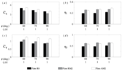
Figure 10. Average side force coefficient  (a), average thrust coefficient
  (c), and two definitions of efficiency,
  (b) and
  (d), over a cycle as functions of the plate kinematics for plates
  ,
,  , and
, and  . The x-axis indicates the stroke angle ϕ on the top row and the stroke time ts on the bottom row.
Download figure:
Standard image High-resolution imageFrom figures 9(d)–(f), the significant increase in thrust during both strokes is apparent as plate  increases the peak thrust by
  on average compared with plate
  . It should be noted that the flat region immediately preceding the peak in CT corresponds to the period of time when snap-buckling occurs; during this transition from one curved geometry to another, the thin polycarbonate sheet is completely passive to the flow, so no additional force is generated. However, snap-buckling is an abrupt process causing the peaks in CS shown in figures 9(a)–(c). Plate
  increases the peak side force by 47.6% on average compared with plate
  . The results from the instantaneous
  in figures 9(g)–(i) corroborate the results from CS. Overall, plate
  increases
  per cycle by 34.8% but causes
  to approach that generated by the baseline flat plate, which increases
  and
and  by 30.1% and 23.6%, respectively, compared with plate
  . These results show that using a snap-buckling design can successfully take advantage of an increased thrust during both the forward and the backward strokes with the added benefit, compared with a rigid curved design, that no net side force should be generated as the geometry presented into the flow is identical during both strokes.
3.6. Dye visualization and DPIV
Dye visualization is used to provide qualitative insight into the flow structures generated by plates  and
and  to investigate possible sources for plate
  's significantly increased thrust and efficiency compared to that of plate
  . Plate
  is effectively rigid during each stroke and therefore no dye visualization is provided for the first forward stroke as the generated flow field would be nearly identical to that of plate
  . The first forward stroke is investigated to highlight the effect of the plate's geometry without the influence of a previously generated flow field. The locations of the dye injection points are concentrated near the tip of the plates because the flow is similar on the pressure side of the two plates at locations closer to the pitching axis. Although not visualized, flow at locations closer to the pitching axis simply move in the chord-wise direction away from the centreline towards the edge of the plate. This flow rolls up into an edge vortex that tends to follow the trajectory of the pitching plate as expected from DDPIV studies of a flat plate by Kim and Gharib [10]. This behavior is also exhibited by plate
  because the curvature at locations closer to the pitching axis is small compared to that near the tip of the plate.
Representative snapshots of the generated 3D flow field near the tip of plates  and
and  pitching with a 60° stroke angle and a 1 s stroke time are shown in figure 11. The flow behaves in a similar manner as that from other kinematic sets. From the dye visualization of plate
  in figures 11(a)–(c), the dye originating from the two injection points closest to the tip shows a developing tip vortex which tends to follow the trajectory of the pitching plate with minimal outwards motion. The dye originating from the other two injection points shows a chord-wise flow away from the centreline, taking the most direct path towards the edge of the plate, as expected from studies by Kim and Gharib [10]. From the dye visualization of plate
  in figures 11(d)–(f), the dye originating from the two injection points closest to the tip shows a smaller developing tip vortex which almost immediately sheds by
  0.25 and appears to transition into a shape similar to a vortex ring by
  0.33. The dye originating from the other two injection points shows a flow moving towards the tip of the plate instead of the edge of the plate as seen with plate
  . Additionally, the influence of the geometry moves this flow towards the centreline of the plate to eventually supplement the development of the tip vortex. Compared to plate
  , the geometry of plate
  appears to cause the tip vortex to shed earlier and travel further downstream. Furthermore, this geometry appears to 'channel' the flow near the tip of the plate, causing the dye to move towards the tip rather than the edge of the plate. The early separation of the tip vortex of plate
  may have been influenced by the increased spanwise flow near the tip, due to the geometry of the plate, or the induced velocity of the edge vortices which attach at an angle on the suction side of the plate.
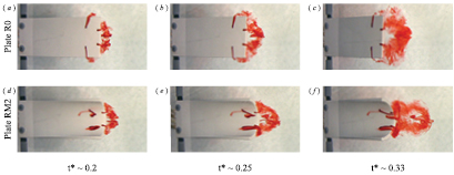
Figure 11. Dye visualization of the flow near the tip of plates  (a)–(c) and
  (d)–(f) from four injection points during the first forward stroke. Snapshots are taken at a t* of approximately 0.2 (a) and (d), 0.25 (b) and (e), and 0.33 (c) and (f). The plates move out of the page with
  at ts = 1 s and are filmed from a location normal to the initial position of the plates to provide a better view of the vortex structures generated behind the plates.
Download figure:
Standard image High-resolution imageDPIV is used to provide quantitative preliminary insight into the mechanism that increases the thrust and the efficiency of plates  and
and  compared with those from plate
  at
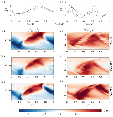
at  60° and ts = 1 s. The flow behaves in a similar manner as that from other kinematic sets. This 2D visualization technique involves high speed imaging of the illuminated particles following the flow. The laser sheet is illuminated along the mid-plane of the plate, indicated by the dashed line in figure 3, where 3D effects are minimal. Evolution of the wake in time is illustrated in figure 12 by first phase averaging the flow field based on the pitching frequency of the plate after reaching steady state, then selecting a single line along the x-direction at a fixed y-location, and finally plotting the velocity field along this line at every instance in time. The line in the x-direction at a fixed y-location is taken at a distance of 1.17 times the span from the pitching location of the plate. The orientation of the pitching motion in figure 12 is identical to that shown in figure 1(b) and, relative to this orientation, flow in the positive x-direction corresponds to a positive U*, while flow in the negative y-direction corresponds to a positive V*. The corresponding phase averaged force data for the generated flow field is shown in figures 12(a) and (b); the positive direction of the forces is denoted by the axes in figure 1(b). The non-dimensional component of velocity in the direction of CS and CT,
  and
and  , respectively, along a line as functions of t* and x* = x/L, where
  is the excursion amplitude of the plate's tip, are shown in figures 12(c)–(h). From figure 12, the U* velocity field generated by all of the plates appears similar, which is reasonable, as CS is similar between all three plates. Additionally, no obvious event in the flow history is linked with the peak in CS for plate
  , which implies that these peaks are primarily due to an abrupt snap-buckling motion rather than a flow phenomenon.
Figure 12. Phase averaged CS (a) and CT (b) with their corresponding phase averaged flow fields, U* ((c), (e), (g)) and V* ((d), (f), (h)), respectively, from a 60° stroke angle and a 1 s stroke time after reaching steady state as functions of x* and t*. Visualization of the flow field is created by plotting the velocity profiles in time along a selected line in the x-direction at a fixed y-location from the near wake of the pitching plates. The orientation of the pitching motion is identical to that shown in figure 1(b). Relative to the orientation in figure 1(b), flow in the positive x-direction corresponds to a positive U*, while flow in the negative y-direction corresponds to a positive V*. Panels (c) and (d), (e) and (f), and (g) and (h) correspond to the flow field generated by plates  ,
,  , and
, and  , respectively, as indicated on the right of panels ((d), (f), (h)), respectively.
Download figure:
Standard image High-resolution image
Comparison of the V* velocity field between the three plates illustrates a possible cause of the improved thrust performance of plate  . Compared with plate
  , plate
  generates a V* velocity field of a significantly greater magnitude. From a simple momentum argument, the greater the momentum imparted to the flow, the greater the thrust generated. The large thrust peaks of plate
  are a result of the dark red regions in figure 12(h). Within these regions, the flow is almost impulsively 'channeled' outwards from the plate in the spanwise direction immediately following snap-buckling, illustrated by the abrupt change in color around a t* of 0.2 and 0.7; the peak in CT appears in the force measurements before the corresponding event in the flow because the recently-imparted momentum into the flow has to convect to the line where the velocity field is sampled.
A similar 'channeling' effect is present during the forward stroke of plate  in figure 12(f). Immediately following a change in direction, when a concave geometry is presented into the flow around t* = 0.2, a red concentrated region appears, but with a smaller magnitude than that from plate
  because no abrupt snap-buckling occurs. However, when a convex geometry is presented into the flow during the backward stroke, the V* velocity approaches and even decreases below zero, which explains the poor thrust performance of the rigid curved geometries during the backward stroke, as described in sections 3.1 and 3.3. It should be noted that the velocity field interestingly resembles a pulsing flow, as most of the thrust is generated during the forward stroke followed by a 'recovery' phase during the backward stroke. Overall, these results suggest that the peak in CS for plate
  is caused by the abrupt snap-buckling motion and that the increase in thrust during the forward stroke of plate
  and both strokes of plate
  may have been caused by a 'channeling' effect where the incoming flow is redirected outwards from the plate in the spanwise direction. A definitive answer regarding the underlying mechanisms requires future studies with a quantitative 3D flow visualization technique.
3.7. Conclusions
The effect of chord-wise tip curvature on the hydrodynamic forces was tested with flapping plates of different geometries. The first case study involved the impact of physically bending the two corners of a plate towards each other. From the baseline study using rigid curved geometries, the results suggested that increasing the curvature decreases the hydrodynamic forces and torques with a minimal loss in efficiency. This concept was explored using a plate with a dynamically-actuated chord-wise tip curvature using a Nitinol wire, which corroborated the result from the baseline study with the added benefit that the amplitude and the duration of the decrease in forces could be arbitrarily modulated.
The second case study involved isolating the impact of chord-wise tip curvature by using plates with a similar planform area to that of the baseline flat plate. Similar to the previous case study, increasing the curvature decreased the generated forces and torques, with the exception that the thrust generated during the forward stroke increased. This benefit was leveraged using a snap-buckling plate to present a concave geometry into the flow during both the forward and the backward strokes, which significantly increased the overall thrust generated per cycle. Investigation through dye visualization and DPIV suggested that this increase in thrust may have been due to a 'channeling' effect, where the incoming fluid is redirected outwards from the tip of the plate rather than moving around it as a result of the geometry of the plate, imparting more momentum to the flow in the thrust direction. Future studies using a quantitative 3D flow visualization technique will be necessary to provide a more definitive answer regarding the underlying mechanisms.
These results suggest that two new mechanisms could potentially be used to increase the maneuverability or the efficiency of AUVs. If the goal is improved maneuverability, implementing actuated chord-wise tip curvature shows promise to assist in braking and turning without needing to modify the trajectory. If the goal is improved efficiency, replacing a rigid flat plate propulsor with a snap-buckling plate of a similar planform area shows promise to achieve this goal, provided the angular velocity of the plate is sufficient to snap-buckle the material.
Acknowledgments
This work was supported by the Charyk Bio-inspired Laboratory at the California Institute of Technology. NM was supported by the National Science Foundation Graduate Research Fellowship under Grant No. DGE-1144469. The plates used for dye visualization were fabricated at the Caltech Library TechLab 3D Printing Facility, which was created and is sustained by funding from both the Caltech Moore-Hufstedler Fund and the Caltech Library.