Article

New Evidence of Mediterranean Climate Change and Variability from Sea Surface Temperature Observations

by
Andrea Pisano
1,*,
Salvatore Marullo
1,2,
Vincenzo Artale
1,2,
Federico Falcini
1,
Chunxue Yang
1,
Francesca Elisa Leonelli
1,3,
Rosalia Santoleri
1 and
Bruno Buongiorno Nardelli
4
1
Consiglio Nazionale delle Ricerche, Istituto di Scienze Marine (CNR-ISMAR), 00133 Rome, Italy
2
Agenzia Nazionale per le Nuove Tecnologie, l’Energia e lo Sviluppo Economico Sostenibile (ENEA), Centro Ricerche Frascati, 00044 Frascati (Rome), Italy
3
Dipartimento di Matematica, Sapienza Università di Roma, 00185 Rome, Italy
4
Consiglio Nazionale delle Ricerche, Istituto di Scienze Marine (CNR-ISMAR), 80133 Naples, Italy
*
Author to whom correspondence should be addressed.
Remote Sens. 2020, 12(1), 132; https://doi.org/10.3390/rs12010132
Submission received: 25 November 2019 / Revised: 20 December 2019 / Accepted: 24 December 2019 / Published: 1 January 2020
(This article belongs to the Special Issue Sea Surface Temperature Retrievals from Remote Sensing)

Abstract

:
Estimating long-term modifications of the sea surface temperature (SST) is crucial for evaluating the current state of the oceans and to correctly assess the impact of climate change at regional scales. In this work, we analyze SST variations within the Mediterranean Sea and the adjacent Northeastern Atlantic box (west of the Strait of Gibraltar) over the last 37 years, by using a satellite-based dataset from the Copernicus Marine Environment Monitoring Service (CMEMS). We found a mean warming trend of 0.041 ± 0.006 C/year over the whole Mediterranean Sea from 1982 to 2018. The trend has an uneven spatial pattern, with values increasing from 0.036 ± 0.006 C/year in the western basin to 0.048 ± 0.006 C/year in the Levantine–Aegean basin. The Northeastern Atlantic box and the Mediterranean show a similar trend until the late 1990s. Afterwards, the Mediterranean SST continues to increase, whereas the Northeastern Atlantic box shows no significant trend, until ~2015. The observed change in the Mediterranean Sea affects not only the mean trend but also the amplitude of the Mediterranean seasonal signal, with consistent relative increase and decrease of summer and winter mean values, respectively, over the period considered. The analysis of SST changes occurred during the “satellite era” is further complemented by reconstructions also based on direct in situ SST measurements, i.e., the Extended Reconstructed SST (ERSST) and the Hadley Centre Sea Ice and Sea Surface Temperature dataset (HadISST), which go back to the 19th century. The analysis of these longer time series, covering the last 165 years, indicates that the increasing Mediterranean trend, observed during the CMEMS operational period, is consistent with the Atlantic Multidecadal Oscillation (AMO), as it closely follows the last increasing period of AMO. This coincidence occurs at least until 2007, when the apparent onset of the decreasing phase of AMO is not seen in the Mediterranean SST evolution.

Graphical Abstract

1. Introduction

Sea surface temperature (SST) is one of the essential climate variables (ECVs), as defined by the Global Climate Observing System (GCOS): it plays a key role in regulating climate and its variability. SST modulates the exchange of heat between the ocean and the atmosphere, and reflects, together with sea surface salinity, the modifications of the thermohaline motions in the ocean.
From seasonal to longer timescales (i.e., interannual, decadal, and multidecadal), SST responds to both natural climate variability [1] and human-driven climate change [2]. SST annual cycle is the dominant oscillation induced by the solar forcing. However, the annual cycle is not the sole regular response to the solar radiation as is modulated by other external environmental factors, such as changes in wind forcing [3], cloudiness [4], and ocean–atmosphere interactions [5]. Also, on seasonal timescales, a change in the seasonal amplitude/phase can substantially contribute to the interannual variability in mean temperatures [6]. On interannual and (multi-)decadal timescales, the nonseasonal or slow variation in SST is modulated by atmospheric and oceanic circulation variability that leads to quasi-periodic oscillations and/or dominant patterns. Examples include the interannual fluctuations in the eastern equatorial Pacific mean SST, identified with the El Niño Southern Oscillation (ENSO) [7], a tripole of SST anomalies in the North Atlantic [8] associated to the North Atlantic Oscillation (NAO) [9], and the multidecadal SST fluctuation in the North Atlantic domain associated to the Atlantic Multidecadal Oscillation (AMO) [10]. On the other hand, increased concentration of atmospheric greenhouse gases have altered the Earth’s energy balance, resulting in the accumulation of thermal energy in the climate system [11]. During the past fifty years more than 90% of this extra energy has been accumulated into the oceans with a primary consequence of raising SSTs [12]. Indeed, from the beginning of the 1970s, a global mean surface temperature (including land surface temperature) warming trend became evident “beyond the bounds of natural variability” [11]. SST is thus a key parameter to track climate change, monitor and characterize the state of the global climate system and contribute to the definition of the present state of the oceans, at both global and regional scales.
At regional scale, the Mediterranean Sea plays a role of the sentinel (hotspot) of global warming since it responds to climate change [13]. Indeed, the Mediterranean was one of the first seas where a warming trend of the deep water temperatures in the western basin was attributed to global warming [14]. The Mediterranean SST has been experiencing an intensive and continuous warming trend since the mid-1980s and this warming tendency is likely projected to increase throughout the 21st century under present climate scenarios [15]. Several studies have shown a consistent increase in the mean Mediterranean SST in the last three decades, taking also advantage of the availability of long-term satellite-based SST data. Based on the 4 km Advanced Very High Resolution Radiometer (AVHRR) Pathfinder SST dataset [16], the author of [17] estimated a mean warming trend of 0.03 ± 0.008 C/year in the western Mediterranean Sea and 0.05 ± 0.009 C/year in the eastern basin from 1985 to 2006. Analogous results were obtained in [18], where a mean warming trend of 0.031 ± 0.003 C/year in the western Mediterranean Sea from 1985 to 2007 was found. These authors [18] also evidenced a significant seasonal variability in the SST trend, observing the highest warming rate in spring, approximately 0.065 ± 0.012 C/year, and much lower warming rates, approximately 0.02 C/year or less, during the other three seasons. Based on Reynolds’ SST reanalysis [19], a satellite-based gap-free (optimally interpolated) SST dataset on a 0.25 grid, the authors of [20] found a mean warming trend of 0.035 ± 0.007 C/year during a 31-year period (1982–2012) over the Mediterranean Sea, ranging from 0.016 ± 0.001 C/year in winter to 0.038 ± 0.109 C/year in spring.
More recently, using the same dataset, the authors of both [21] and [22] estimated a mean warming trend of ~ 0.036 C/year for the whole Mediterranean Sea, although looking at different periods: from 1993 to 2017 and from 1982 to 2016, respectively. The authors of [23] investigated decadal variability in the Mediterranean SST on a 24-year period (1985–2008), making use of a regionally optimized satellite-based SST dataset over the Mediterranean Sea [24] and in situ-based SST data. These authors [23] estimated a mean warming trend of ~ 0.037 C/year for the whole Mediterranean Sea, ~ 0.026 C/year for the western basin and ~ 0.042 C/year for the eastern basin. Between 1985 and 2008, these authors [23] also evidenced a marked seasonal variability in the SST trend, estimating a higher warming rate in spring (~ 0.054 C/year) and summer (~ 0.044 C/year) than in autumn (~ 0.027 C/year) and winter (~ 0.023 C/year).
The analysis of the spatial patterns of the Mediterranean SST trend has showed a marked difference between the western and eastern Mediterranean. The authors of [23] evidenced two main periods, before and after 1990, during which the two sub-basins showed opposite trend patterns. They suggest that the 1985–1990 period might be regarded as a transition period, after which the observed trend pattern reversed, with an initial warming trend in the western Mediterranean and a cooling trend in the eastern basin until 1990. The authors of [25] found a similar pattern of eastward increasing trend in the Mediterranean SST since the early 1990s. In addition, the authors of [23] pointed out that the shift (from westward to eastward) coincided with a change from a high positive to a low NAO phase, thus suggesting a potential link between NAO and SST variations on decadal timescales. Furthermore, throughout the period 1973–2008, the same authors evidenced a high correlation between AMO and the first temporal mode of the Mediterranean SST anomalies, the latter associated with the long-term SST trend.
Among the natural modes of climate variability, NAO and AMO are particularly relevant for the Mediterranean climate. NAO is the dominant pattern of wintertime atmospheric circulation variability over the extra-tropical North Atlantic domain [9]. The decadal oscillation of the sea level pressure (SLP) anomalies is followed by wind, air temperature, and precipitation changes, especially in winter and early spring [26], over the North Atlantic and across Europe, including the Mediterranean Sea. In particular, a positive phase of NAO is associated with warmer conditions over the western Mediterranean and cooler conditions over the eastern basin, whereas the contrary occurs during negative phases.
AMO can be defined in several but similar forms. According to the definition in [27], the 60 S–60 N SSTs are subtracted from the North Atlantic SSTs while the North Atlantic SSTs (0–70 N) are simply detrended following the [28] definition. AMO is particularly relevant for the North Atlantic-Mediterranean system [29]. Indeed, according to the authors of [23,30,31], the Mediterranean SST shows multidecadal AMO-like variability, with over 30% of explained variance. In particular, the authors of [31] evidenced the presence of a significant oscillation in the Mediterranean SST with a period of approximately 70 years, very close to the AMO index. However, the nature/origin of this Mediterranean AMO variability is still a matter of debate, concerning the existence of a dynamical linkage transmitting the AMO signal from the Atlantic to the Mediterranean (e.g., anomalous heat advection processes or cloud-related processes).
Herein we analyze the variability in the Mediterranean SST and the adjacent Northeastern Atlantic box (west of Gibraltar) from seasonal to decadal timescales. We provide updated trend estimates for the whole Mediterranean Sea, its main sub-basins (i.e., western Mediterranean Sea, Adriatic Sea, Ionian Sea, and Levantine–Aegean Sea), and the Northeastern Atlantic box, making use of the most recent satellite SST dataset over the Mediterranean Sea (1982–2018). In addition, by using two long-term in situ-based SST reconstructions, covering the last 165 years, we analyze the Mediterranean multidecadal SST variability in relation to AMO. Specifically, in the framework of the Copernicus Marine Environment Monitoring Service (CMEMS), the Satellite Oceanography Group of the Italian National Research Council (CNR-GOS) has recently produced an updated version of the Mediterranean optimally interpolated SST dataset [32]. This is a satellite-based dataset which provides daily (nighttime) 4-km resolution optimally interpolated SST data from 1982 to 2018 over the Mediterranean Sea and the Northeastern Atlantic box. Indeed, even if there is a variety of historical SST datasets available (e.g., Reynolds v.2 reanalysis [19], Operational SST and Sea Ice Analysis (OSTIA) [33], and European Space Agency’s Climate Change Initiative (ESA-CCI) SST dataset [34]), this dataset provides the longest record of foundation temperature (namely, the temperature below the layer affected by the diurnal cycle [35]) interpolated fields at high resolution (4 km), with relatively high accuracy (root mean square error of ~ 0.58 C when compared with in situ data) obtained by a regionally optimized processing. Longer time series but at lower spatial and temporal resolution are provided by the Extended Reconstructed SST (ERSST, monthly 2 × 2 degrees spatial resolution, 1854–today) [36] and by the Hadley Centre Sea Ice and Sea Surface Temperature dataset (HadISST, monthly 1 × 1 degrees spatial resolution, 1870–today) [37].

2. Materials and Methods

2.1. SST Covering the Satellite Era: CMEMS Mediterranean Dataset

Satellite observations have the unique capability (compared to in situ measurements) to provide systematic global and/or regional SST synoptic coverage at high spatial and temporal resolution, i.e., from one to a few kilometers and from hourly to daily frequency. SST has been measured from space over cloud free areas with relatively high accuracy (~0.5 C) with the first 5-channel Advanced Very High Resolution Radiometer (AVHRR) since late 1981 [38].
The Pathfinder program [16], established in 1990 as a NOAA/NASA project, provides a consistent, accurate and long-term satellite-based SST dataset for global climate applications. Since 1990, the Pathfinder program has produced five versions of the so-called 4 km AVHRR Pathfinder dataset, which is a reprocessed SST dataset built using the whole second-generation AVHRR sensors onboard the NOAA polar-orbiting satellites. The latest AVHRR Pathfinder release, i.e., v.5.3 (PFV53), consists of global, daily (available as nighttime and daytime data) 4 km resolution non-interpolated (also known as Level-3 collated, L3C, following the Group for High Resolution SST, GHRSST, definitions) data from 1981 to 2014 and represents the longest global SST dataset from space.
Taking advantage of PFV53, in the framework of CMEMS, the CNR-GOS has produced a long-term (1982–2015), daily (nighttime) 4 km resolution optimally interpolated (Level-4, L4) SST dataset covering the Mediterranean Sea, hereafter referred to as CMEMS Mediterranean SST dataset. The daily SST fields correspond to gridded optimally interpolated AVHRR PFV53 L3C nighttime data, then representative of the foundation temperature and are freely distributed through CMEMS, identified as SST_MED_SST_L4_REP_OBSERVATIONS_010_021. In the CMEMS Mediterranean dataset, SST data have been interpolated on the original Pathfinder grid and are representative of night SST values (00:00 UTC). The interpolation of PFV53 L3C data (1982–2015) to L4 has been carried out by adapting the CNR-GOS near-real-time (NRT) SST processing chain [39] to the PFV53 dataset.
As PFV53 data end in 2014, a bias-corrected version of the CMEMS NRT Ultrahigh Resolution (UHR) L4 product for the period 2015–2018 (identified as SST_MED_SST_L4_NRT_OBSERVATIONS_010_004 in the CMEMS web portal), hereafter recalled as Interim data, has been used to extend the CMEMS reprocessed dataset up to 2018. To build the Interim product, we followed this strategy:
  • Downsize the Mediterranean NRT UHR L4 (1 km) product to the CMEMS Mediterranean dataset grid resolution (4 km).
  • Estimate the differences in terms of bias and root-mean-square error (RMSE) between the two products for the overlap period (2008–2014).
  • Perform a local bias correction of the NRT products from 2015 to 2018.
  • Extension to 2018.
A detailed description of the data processing can be found in [32], and in the Product User Manual (PUM) and Quality Information Document (QUID) available in the CMEMS online catalogue.

2.2. SST Reconstructions Back to the Nineteenth Century: HadISST and ERSST

In situ measurements provide the longest historical SST data records (compared to satellite observations). Herein we use the Met Office Hadley Centre Sea Ice and Sea Surface Temperature dataset (HadISST [37]), and the Extended Reconstructed Sea Surface Temperature (ERSST [36]). The HadISST dataset is a combination of global, spatially complete monthly SST and sea ice concentration fields from 1870 to present. SSTs in HadISST are built using a reduced space optimal interpolation from the Marine Data Bank (mainly ship tracks), the International Comprehensive Ocean–Atmosphere Data Set (ICOADS) through 1981 and a blend of in situ and adjusted satellite-based SSTs from 1982 onwards. HadISST v.1.1 data are distributed at a monthly time step from 1871 to present at 1 × 1 degree resolution. The ERSST dataset provides global, spatially complete monthly SST averages at 2 × 2 degree resolution since 1854 to present. Version 5 (ERSSTv5 [36]), as well as previous version, is based upon statistical interpolation of the ICOADS data. This last version incorporates the last release of ICOADS 3.0, a decade of near-surface data from Argo floats, and a new estimate of centennial sea ice from HadISST.2. ERSST only uses in situ observations.

2.3. Statistical Methods

Monthly mean SST maps were constructed from the daily CMEMS Mediterranean SST data for the period 1982–2018 over the entire domain (Figure 1-A1). Then, the domain was divided in 4 Mediterranean sub-basins, i.e., western Mediterranean Sea (Figure 1-A3), Adriatic Sea (Figure 1-A4), Ionian Sea (Figure 1-A5) and Levantine–Aegean Sea (Figure 1-A6), and the adjacent Northeastern Atlantic box (Figure 1-A2). For each of these areas the spatial average was computed to produce four univariate time series of monthly mean SSTs plus one for the whole Mediterranean Sea and one for the Northeastern Atlantic box.

2.3.1. X-11 Seasonal Adjustment Procedure

Trend analysis has been performed by using the X-11 seasonal adjustment procedure [6], which is briefly summarized herein. Given T t , t = 1 , 2 , , n , an input time series (namely, the time series of monthly mean SSTs), the X-11 procedure generates the following additive decomposition,
X t = T t + S t + I t
where T t is the trend component, S t the seasonal component, and I t the irregular component, which the latter accounts for the residual irregular variations such as subannual fluctuations. The decomposition is obtained through iterative application of different running means, which have the effect of a low-pass filter for Tt estimation and a seasonal filter for St estimation.
The X-11 method is a three-step filtering algorithm, which consists of an alternate trend estimation on the seasonally adjusted time series ( X t S t ) and a seasonal estimation on the trend adjusted series ( X t T t ), using moving averages to estimate both components. Specifically, the first step provides a preliminary estimate of the trend component obtained applying a centered 25-term (two years) moving average ( MA ) to X t , i.e., T t 1 = MA 2 × 24 ( X t ) . Then, a preliminary estimate of the seasonal component is obtained by applying a centered 5-term (i.e., 5 months) seasonal moving average filter ( SMA 3 × 3 ) to the detrended (or trend-adjusted) time series Z t = X t T t 1 , which represents seasonality and shorter-term only, i.e., S t 0 = MA 3 × 3 ( Z t ) . The resulting seasonal component S t 1 is adjusted by subtracting its annual-centered running mean, S t 1 = S t 0 < S t 0 > , producing an approximately zero mean seasonality. The second step provides improved trend and seasonal estimates repeating the first step but applied to the seasonally adjusted series Y t = X t S t 1 as follows; T t 2 = MA 2 × 24 ( Y t ) and S t 2 = MA 3 × 5 ( Z t 1 ) , where MA 3 × 5 is a centered 7-term (i.e., 7 months) seasonal moving average filter and Z t 1 = X t T t 2 the detrended time series. Then, the seasonal component S t 2 is adjusted to have zero mean. The third step produces the final trend estimate, T t 3 = MA 2 × 24 ( Y t = X t S t 2 ) , and finally computes the residual component as I t = X t S t 2 T t 3 , while the seasonal series S t 2 is left unchanged.
Compared to the more (and widely used) traditional approach that treats the annual cycle as a fixed mean effect, which is then subtracted to the time series of SSTs, the X-11 procedure has the advantage of estimating the annual cycle on a year-to-year basis, thus taking into account potential variations in the cycle amplitude.

2.3.2. Trend Estimation

The X-11 method provides a continuous interannual trend signal ( T t ), as shown in Figure 5 by red lines, whose slope gives the trend estimate. Specifically, the trend is computed through a two step procedure: (1) Mann–Kendall (MK) test [40,41] is applied to T t to test whether there is a monotonic upward or downward trend over time (versus the null hypothesis of no trend); (2) Sen’s method [42] is applied to estimate the slope (or trend, C/year) of T t as the median of the slopes of all pairwise differences in T t . MK test has the advantage of being nonparametric (i.e., no assumptions on data distribution) and much less sensitive to outliers and skewed distributions. This method does not require time series to be serially correlated, a condition satisfied since T t does not contain the annual cycle.
Given a time series of n observations, x 1 , , x n , MK test is based on the test statistic S :
S = i = 1 n 1 j = i + 1 n sgn ( x j x i )
with
sgn ( x j x i ) = 1 if ( x j x i ) > 0 0 if ( x j x i ) = 0 1 if ( x j x i ) < 0
where j > i . The mean of S is E [ S ] = 0 and variance Var ( S ) defined as:
Var ( S ) = 1 18 [ n ( n 1 ) ( 2 n + 5 ) p = 1 q t p ( t p 1 ) ( 2 t p + 5 ) ]
where q is the number of tie groups (namely, the set of sample data having the same value) and t p the number of observations contained in the p-th tie group. The statistic S is approximately normal provided that the following Z -transformation is applied:
Z = S 1 Var ( S ) if S > 0 0 if S = 0 S + 1 Var ( S ) if S < 0
Then, chosen the level of significance α , the null hypothesis (no trend) is rejected if | Z | > Z 1 α / 2 , and the alternative hypothesis of increasing ( S > 0 ) or decreasing ( S < 0 ) trend is accepted. Also, according to Z , the p-value is computed.
The magnitude of slope, β , is determined using Sen’s method:
β = Median [ Q k = x j x i j i ] , j > i ; k = 1 , , n ( n 1 ) 2
where Q k is the ensemble of all possible pairs of differences x j x i in the sample.
In this work, the level of significance has been set to α = 0.05 (then, p 0.05 ), so that all the trends provided here are statistically significant at the 95% level. Finally, a bootstrap procedure [43] is used to estimate the 95% confidence interval of the trend (namely, two times the standard deviation as estimated with the bootstrap procedure).

3. Results

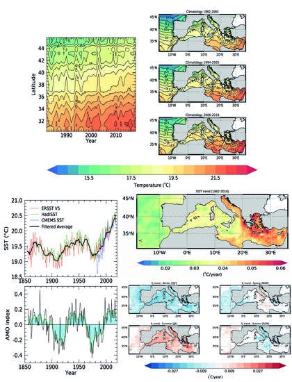
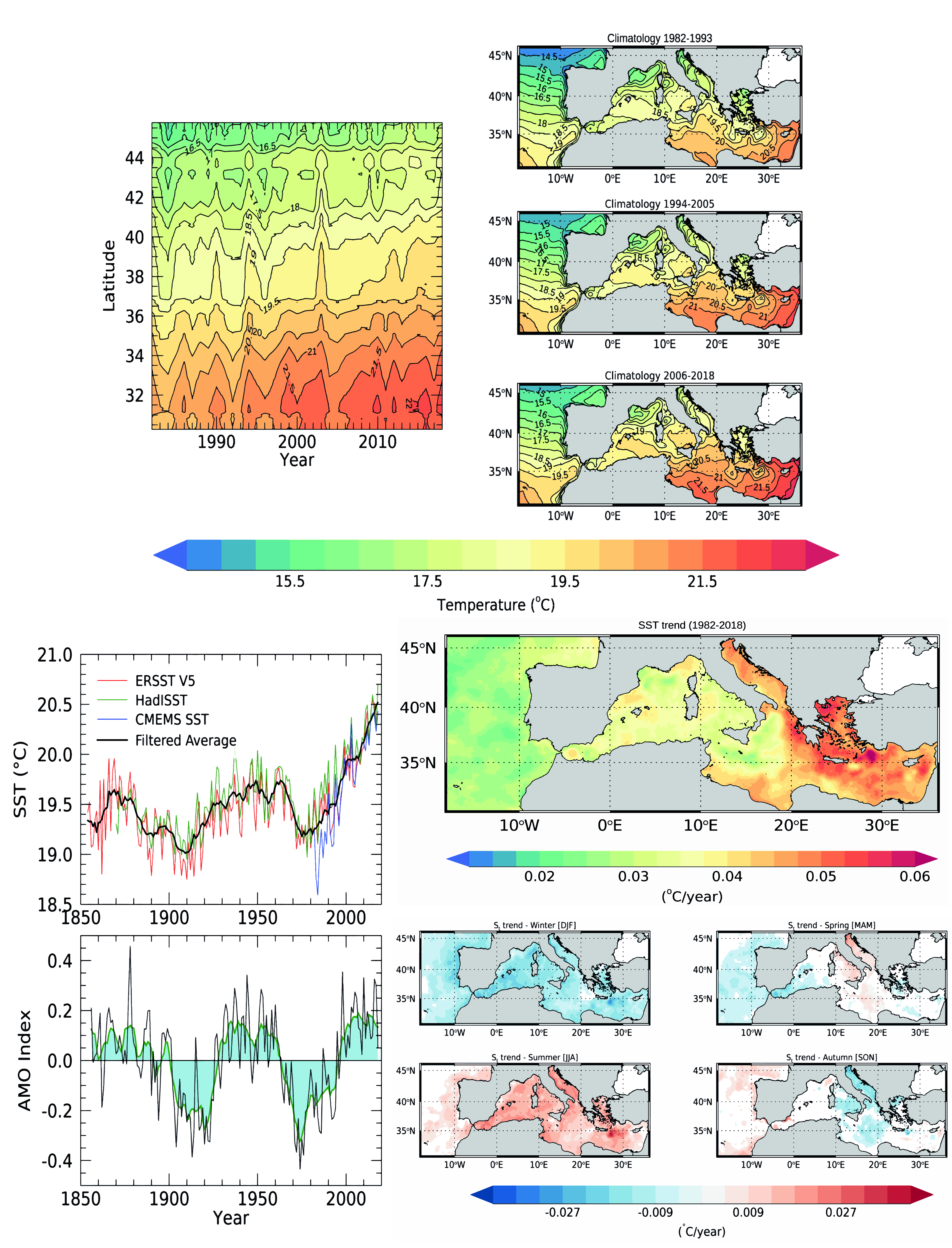
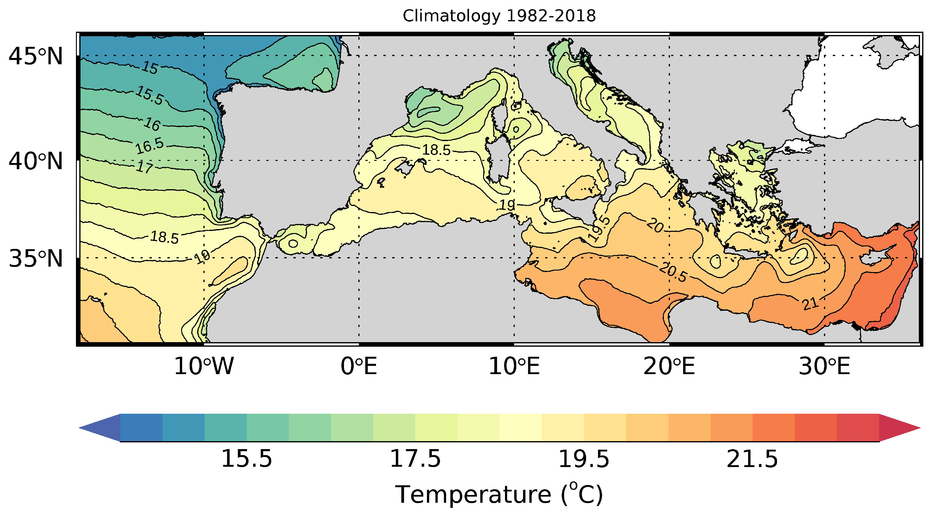
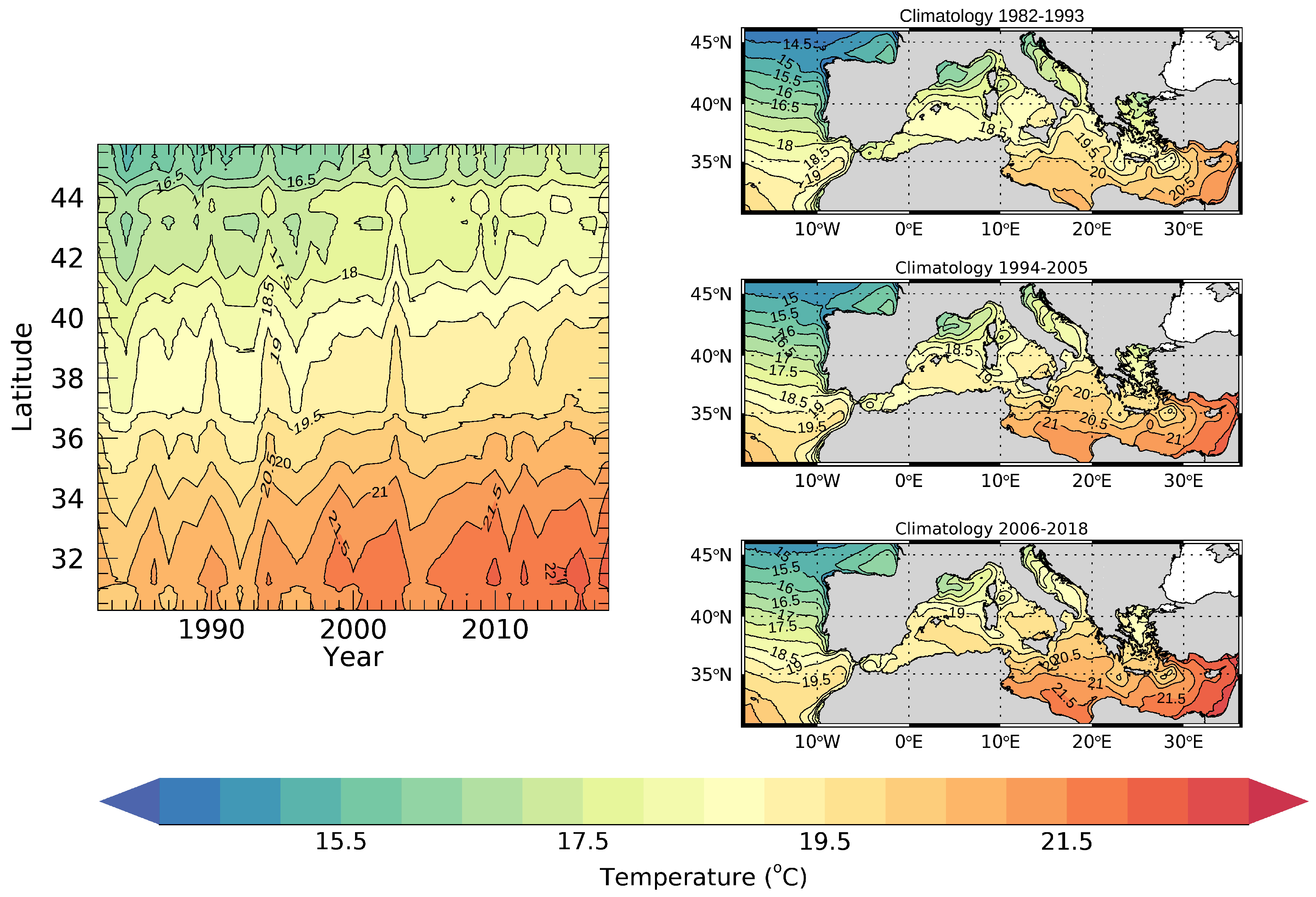
3.1. Mediterranean SST Climatology Patterns

The mean Mediterranean SST field over the period 1982–2018, obtained by averaging all the daily CMEMS SST maps, is shown in Figure 2. As expected, the 1982–2018 SST spatial pattern is characterized by a clear zonal variation, with lower temperatures in the north and higher temperatures in the south. This zonal gradient is, however, modulated by the presence of some of the known mean oceanographic structures [44] that affect the Mediterranean surface temperature [45] (Figure 1). In the eastern Mediterranean Sea, the Western Cretan and the Rhodes gyres are well visible, whereas in the west the relatively colder water in the Gulf of Lion marks the area of cyclonic circulation characterized by winter deep water formation events [46] (see Figure 1 and Figure 2). Cold temperatures in the north Tyrrhenian Sea between Corsica and Italy are the signature of a cyclonic gyre (Figure 1 and Figure 2) due to the interaction of the Mistral with the complex orography in the area between Corsica and Sardinia (Strait of Bonifacio) [47]. In the Alboran Sea, just east of Gibraltar, the thermal signature of the west Alboran Gyre is evident (Figure 1 and Figure 2), whereas the eastern Alboran Gyre is just hinted [48]. In the Atlantic Ocean the cold temperature patterns along the coasts of Portugal [49] and Northwest Africa [50] highlight the presence of the coastal upwelling driven by the seasonally varying Trade Winds.

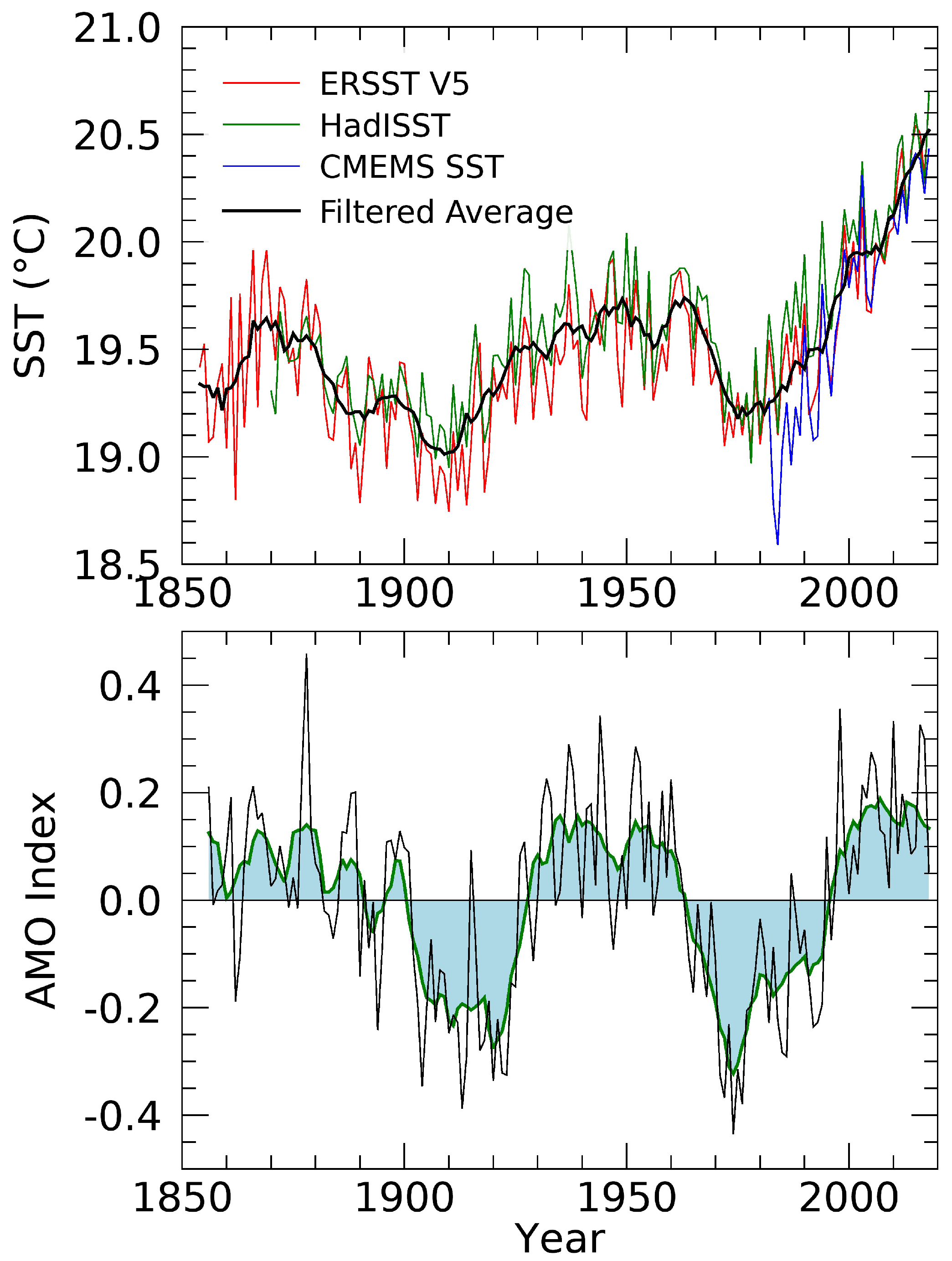
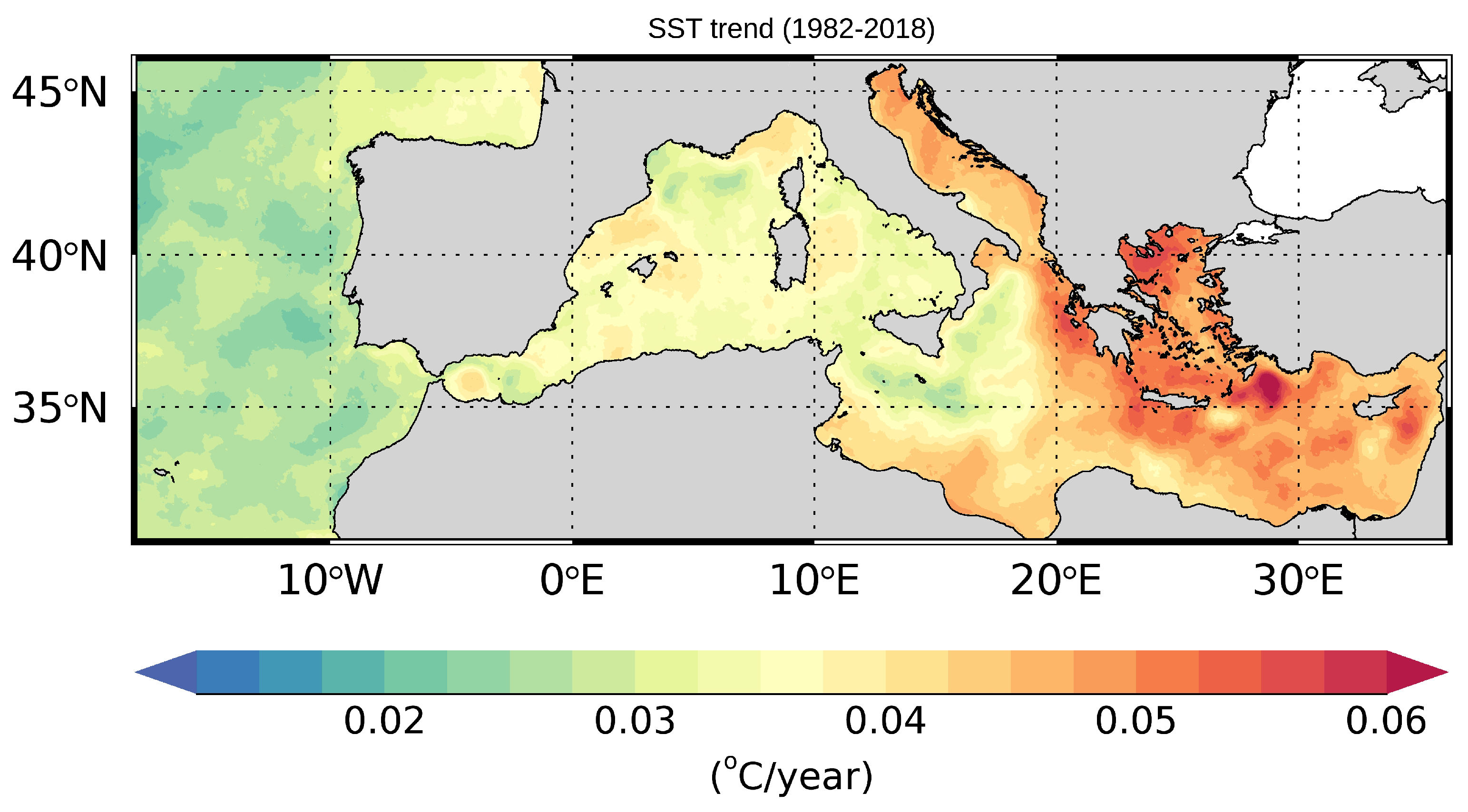
3.2. General Spatial and Temporal Patterns of SST Changes

The time evolution of the Mediterranean mean SST field shows a general warming increase over the entire period (Figure 3). In particular, the annual mean SSTs show a steep increment after 1993, mainly due to the increase of temperature in the southern waters of the eastern Mediterranean Sea (Figure 3): (i) the 21 C isotherm appeared in 1993 and persisted at latitudes initially between 32 and 33 N and, by the end of the period, at latitudes between 34 and 35 N; (ii) the 21.5 C appeared in 1998 and persists until the end of this investigation period, with a single interruption in 2004; and (iii) the 22 C isotherm episodically appears since 2010. Beyond the details, we thus observe a general, northward migration of isotherms since 1993, with isolated peaks that can be associated with extreme marine heatwaves such as those of 2003, 2006, and 2015 [51,52].
This analysis suggests a nonuniform spatial and temporal variability of the Mediterranean SST, with the eastern basin getting warmer more rapidly, compared to the western basin. This is well depicted by dividing the 37-years period into three intervals of approximately 12 years each (Figure 3, right panel). This sequence essentially shows a constant increase of the SST in the three periods; however, this warming is clearly more evident in the eastern Mediterranean Sea with respect to the western side and the Northeastern Atlantic box.
The continuous, nearly monotonic, increase of the Mediterranean annual mean surface temperature corresponds to the increasing phase of the Atlantic Multidecadal Oscillation (AMO unsmoothed from the Kaplan SST V2 calculated at NOAA/ESRL/PSD1; Figure 4). Using the HadISST and ERSST long-term datasets, covering the period from 1854 to present (see Section 2.2), a positive correlation between AMO and Mediterranean SST variability is found, namely, r = 0.65 ( p 0.05 ) between the green (AMO) and black (filtered SST average) curves, Figure 4. This result confirms what was first observed in [31], and then in [23]. However, the comparison between the Mediterranean annual mean SST and the AMO signal during the last decade shows that the linear behavior of Mediterranean SST does not follow the plateau that characterizes the AMO index during this period (Figure 4). Specifically, after 2007, the Mediterranean SST continues to rise linearly while AMO remains substantially constant (in the average) with some tendency to decrease in the last years of the time series.

3.3. Separating Interannual/Decadal SST Variations from Seasonal and Higher Frequency Signals

3.3.1. X11-Trends

The Mediterranean Sea trend component shows a nearly continuous warming trend (Figure 5-A1) at a rate of 0.041 ± 0.006 C/year, interrupted by the 1984, 1992, 1996, and 2005 local minima, accounting for a total SST increase of about 1.5 C from 1982 to 2018; a definitely higher value than the 0.027 ± 0.008 C/year observed in the Northeastern Atlantic box (Figure 5-A2). At sub-basin level, the western Mediterranean and the Ionian Seas show lower trend values respect to the rest of the basin, i.e., 0.036 ± 0.006 C/year and 0.037 ± 0.007 C/year, respectively, though still larger than those of the Northeastern Atlantic box. The most intense warming trends are observed in the Adriatic Sea and in the Levantine–Aegean basin where the warming reached values of 0.045 ± 0.007 C/year and 0.048 ± 0.006 C/year, respectively.
The Mediterranean trends found here are consistent with the results ( 0.04 C/year) obtained in [53] using a shorter (1986–2015) time series. Other recent trends’ estimates provide values of 0.036 ± 0.003 C/year from 1993 to 2017 [21], 0.036 ± 0.003 C/year from 1982 to 2016 [22] and 0.035 ± 0.007 C/year from 1982 to 2012 [20], over the Mediterranean Sea. Trends’ estimates we found in the Mediterranean sub-basins and the adjacent Northeastern Atlantic box agree with previous findings, e.g., the value of 0.031 ± 0.007 C/year from 1985 to 2007 in the western Mediterranean Sea [18], about 0.045 C/year in the Aegean Sea [23] and about 0.025 C/year in the Atlantic area near Gibraltar from 1985 to 2008 [54], about 0.033 C/year in the Ionian Sea and about 0.042 C/year in the Levantine basin from 1982 to 2012 [20]. These trends are quite similar to our estimates within the indicated confidence interval. Differences between these estimates are minimal, considering the different datasets used. Indeed, the authors of [20,21,22] used the gridded daily AVHRR data (version 2) with a 0.25 latitude/longitude resolution, while [53] the previous version of the CMEMS Mediterranean dataset, at 4 × 4 km resolution.
The sub-basins’ description of the time evolution of the Mediterranean SST reflects the occurrence of a nonuniform spatial distribution of the trends, with lower values in the sub-basins closer to the Atlantic Ocean, namely the western Mediterranean and Ionian Seas, and higher values in the Levantine–Aegean Sea and the Adriatic Sea. A more detailed description of the spatial distribution of the SST trend can be obtained by applying the same procedure used for the mean sub-basin SSTs (Figure 5) to each pixel of the SST maps time series (Figure 6). The magnitude of the trend increases moving eastwards, with minima in the Northeastern Atlantic box, in the western basin and Ionian Sea (Strait of Sicily, in particular) and maxima in the eastern Mediterranean Sea, including the Aegean Sea.
Finally, to investigate SST changes on decadal timescales, the spatial pattern of the Mediterranean SST trend has been computed over three periods we depicted in Figure 3, i.e., 1982–1993, 1994–2005, and 2006–2018. In the Mediterranean Sea, each period is characterized by a significant trend: 0.05 ± 0.02 C/year (1982–1993), 0.06 ± 0.02 C (1994–1995) and 0.04 ± 0.01 C/year (2006–2018). In the Northeastern Atlantic box, the first period (1982–1993) shows a strong warming trend of 0.06 ± 0.02 C/year, the second (1994–2005) shows no significant (i.e., p > 0.05 ) trend, and the third period (2006–2018) is characterized by a mild warming trend of 0.03 ± 0.02 C/year.

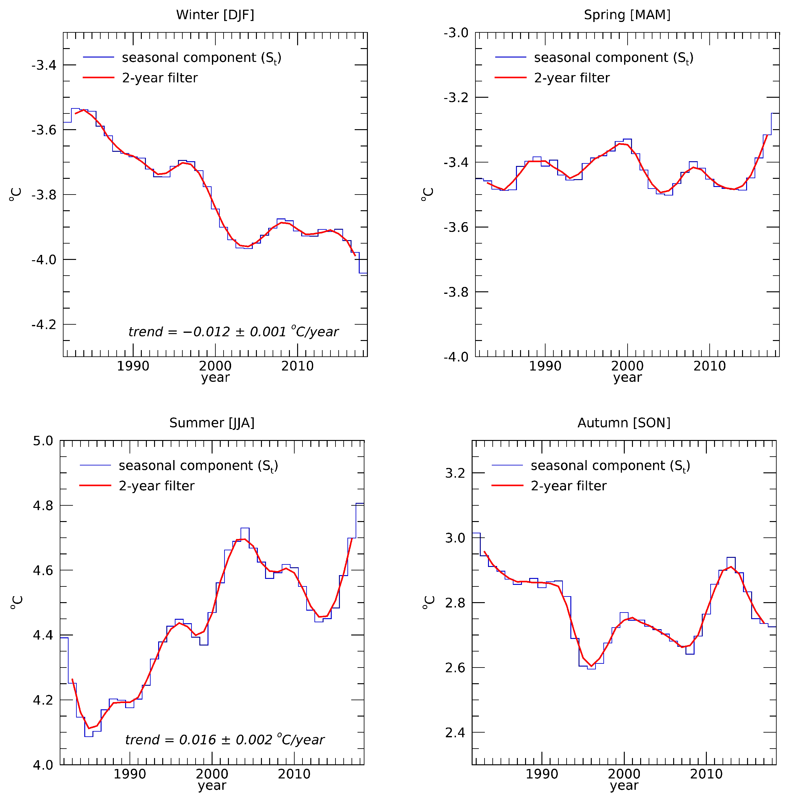
3.3.2. X11-Seasonal Component

Hereafter, we analyze the temporal variability of the seasonal component S t , as deduced from the X-11 analysis. Specifically, we computed separately S t annual mean values over the winter (DJF), summer (JJA), spring (MAM), and autumn (SON) months over the whole Mediterranean, and applied the Mann–Kendall test and Sen’s method to estimate the trend on the resulting time series (Figure 7). As the decomposition provided by X-11 is additive, it is not surprising that the overall warming (provided by T t and discussed in the previous Section 3.3.1) cannot be deduced by comparing the trends estimated from S t component alone. However, noticeably, the summer and winter averaged seasonal component exhibits a significant and opposite trend, estimated in 0.016 ± 0.002 C/year and 0.012 ± 0.001 C/year, respectively. Intermediate seasons do not show a significant trend.
The spatial pattern of the seasonal component trend, estimated per season, is shown in Figure 8; this is because the trend in the seasonal component of the two significant seasons (i.e., winter and summer) is fairly homogeneous over the whole basin, with no positive and negative values in winter and summer, respectively.
In the literature, the change of seasonality is generally deduced from seasonal SST trends, i.e., the trend computed separately for the winter (DJF), summer (JJA), spring (MAM), and autumn (SON) months considering the unfiltered SST data. Then, to provide comparable results, we also estimated the trends following the same procedure applied to the seasonal component (Figure 8) to the sum of the trend and seasonal components (i.e., T t + S t ). The spatial pattern of the SST trend estimated during each season is shown in Figure 9.
The mean SST trends during each season over the whole Mediterranean Sea have been quantified in: 0.029 ± 0.003 C/year (winter), 0.056 ± 0.003 C/year (summer), 0.040 ± 0.003 C/year (spring), and 0.039 ± 0.003 (autumn).

4. Discussion

Mapping changes of regional SST distributions in response to ongoing background warming is an important step towards understanding climate variability and its impacts on weather extremes, marine ecosystem, and related services. SST changes may appear as a shift of the entire distribution (thus showing a trend in the mean values), but also as changes in the shape of the distribution [55]. The CMEMS Mediterranean SST time series, covering the satellite era, is actually displaying both a significant long-term trend and a strengthening of the seasonal cycle. Indeed, comparing the CMEMS satellite-based data to the longer HadISST and ERSST timeseries, we found that the Mediterranean warming trend from 1982 to 2018 is approximately 3.7 times higher than the global ocean warming trend from 1980 to 2005 (=0.011 C/year, [12]).
Noticeably, although the Mediterranean SST trend shows a continuous warming trend, the decadal and spatial analysis (Section 3.3.1) of SST variations evidenced that the warming rate is not uniform, neither in time nor in space. Specifically, three main periods have been identified: 1982–1993 (first period), 1994–2005 (second period), and 2006–2018 (third period). During each period, the Mediterranean SST trend has been estimated in 0.05 ± 0.02 C/year (1982–1993), 0.06 ± 0.02 C/year (1994–1995) and 0.04 ± 0.01 C/year (2006–2018). After an initial, short cooling trend (1982 to ca. 1984), the first period is characterized by a warming phase, from 1985 to 1990, followed by a cooling until the beginning of 1993. From 1993, the second period begins with a strong increase in SST until 1995 and, after a short cooling between 1995–1996, it continues with a warming trend till 2003, where a cooling trend begins, lasting until 2005. The third period shows a continuous warming trend, with no cooling or pausing phases. The first two periods are thus characterized by an alternate warming and cooling tendency, while the third one seems to show an overwhelming warming tendency, at least until 2018.
Regarding the Northeastern Atlantic box, the decadal variability is more pronounced than that of the Mediterranean. Indeed, whereas the first period (1982–1993) evidences a strong warming trend ( 0.06 ± 0.02 C/year), the second one (1994–2005) does not present a statistically significant trend (i.e., no trend at p 0.05 ). Finally, the third period (2006–2018) experiences a mild warming trend of 0.03 ± 0.02 C/year, which is more than twice smaller than the first period trend. Overall, the Mediterranean Sea and the adjacent Northeastern Atlantic box warmed at about the same rate from 1982 to the late 1990s. From 1999 onward, although the trend continues to be positive in the Mediterranean Sea, it slows down in the Northeastern Atlantic box.
Our satellite-based analysis has been compared to the reconstructed HadISST and ERSST data and to the AMO index in order to frame the Mediterranean SST variability, as observed during the satellite era, in a larger time window, i.e., the last two centuries. Past studies [23,30,31] have already highlighted the high correlation between AMO and the Mediterranean SST. The authors of [31] showed a multidecadal AMO-like Mediterranean SST variability throughout the longest currently available period (i.e., 1854 to present). Other works [56,57] indicated that AMO is currently in a modest warming phase. Our analysis shows that the pause of the increasing tendency of AMO since 2000 is captured by the slowdown in the Northeastern Atlantic box SST trend while it is not followed by the Mediterranean SST (Figure 4). The nature/origin of this Mediterranean AMO-like variability is still a matter of debate and investigation. As potential sources of this AMO-like variability, the authors of [23] suggest the influence of the Atlantic inflow on the Mediterranean SST variability through the advection of heating from Gibraltar, whereas the authors of [31] hypothesize either an atmospheric origin or an internal variability related to the Mediterranean Thermohaline Circulation (THC), in analogy to what proposed by [58] for the North Atlantic. Our analysis of the Mediterranean SST variability opens a further question concerning the bifurcation between AMO and Mediterranean SST at the beginning of this last millennium (2000–today).
The spatial pattern of the Mediterranean SST trend also displays a marked difference between its western and eastern basins (Figure 6). These patterns have been suggested to depend on different teleconnections: the west being under the NAO [23] and the east under the South Asian Monsoon influence (e.g., [59]). Regarding mesoscale patterns, the SST trend map (Figure 6) shows some evidence on the fact that SST trend patterns overlay some mean oceanographic Mediterranean structures [20] (e.g., West Alboran Gyre, West Cretan Gyre, Ierapetra Gyre, Rhodes Gyre, and the Tyrrhenian Gyre; see Figure 1 and Figure 6). Moreover, we find minimum trend values in some areas that are characterized by a thick upper mixed layer or recurrent deep convection (e.g., in the Gulf of Lion; see Figure 1 and Figure 6). However, the general SST trend spatial pattern does not overlay with both climatological mixed layer depth and seasonal thermocline depth [60]. This suggests that spatial differences in the warming cannot be solely explained by the distribution of the excess of heat over a larger vertical layer, but rather it opens to hypothesize an effective role of mean circulation and local mean air–sea heat fluxes on SST variability (see Figure 1 and Figure 6).
A relevant seasonal variability and strong positive and negative anomalies, superimposed to the Mediterranean SST trend, are clearly detected in the CMEMS SST dataset (see Section 3.3.2). Indeed, a change of the seasonal cycle amplitude is identified by a significant positive ( 0.016 ± 0.002 C/year) and negative ( 0.012 ± 0.001 C/year) trend of the seasonal component during summer (JJA) and winter (DJF), respectively, whereas no trend during spring (MAM) and autumn (SON) is observed. This gives rise to an increase of the SST trend in summer (about 0.056 C/year), and to a slowdown in winter (~0.029 C/year). No impact is observed in spring and autumn, where the trend (~0.040 C/year) matches the mean annual trend (0.041 C/year). In previous works [18,22,23], a change in the seasonal cycle was generally deduced from a change in the mean trend when computed over the season months. The authors of [18], in their analysis of satellite-based SST observations from 1985 to 2007 in the western Mediterranean, evidenced a significant change in the mean annual trend (about 0.03 C/year) from April to June, estimated in about 0.06 C/year. Over the two decades, these authors found an increase of the mean SST of April, May and June by nearly 1 C, suggesting a lengthening of summer and an advance of summer onset in late spring. The authors of [23] also evidenced a marked seasonal variability in the mean annual trend in the whole Mediterranean (about 0.037 C/year from 1985 to 2008), ranging from 0.054 C/year in spring (MAM) and 0.044 C/year in summer (JJA), to 0.027 C/year in autumn (SON) and 0.023 C/year in winter (DJF).
Changes in seasonal variability affect not only the SST trend during summer and winter seasons (Figure 9), that is, higher warming in summer than in winter, but could also induce an amplification of marine heatwave events, in terms of frequency, magnitude and duration, which in turn can have a vast range of adverse impacts on marine ecosystems [51,52]. Indeed, a marine heatwave has been defined as “a prolonged discrete anomalously warm water event that can be ascribed by its duration, intensity, rate of evolution, and spatial extent” [52]. Based on our analysis (Figure 5), from 2000 the Mediterranean Sea featured the highest SSTs, some of which classified as strong marine heatwaves [51,52]. The signature of the well-known marine heatwave occurred in 2003 is indeed clearly visible in the western Mediterranean basin, the Ionian Sea, and the Adriatic Sea (Figure 5). This extreme warming event lasted for the whole month of June and the summer mean SST anomaly was almost 2 C higher than the climatology [52]. We notice, moreover, that there is no signal of the 2003 warm surface water anomaly in the Northeastern Atlantic Box (Figure 5).
In general, from the beginning of the 2000s, the Mediterranean Sea experienced the highest temperatures and an overwhelming SST trend (Figure 5) along with strong marine heatwaves, well described also in terms of their biological impacts in [51,52]. In addition, warmer SSTs could facilitate (atmospheric) heat waves events. The authors of [61] suggest that the strong increase in SSTs along coasts could impact the sea breeze circulation, which is driven by the land-sea thermal contrast, with the consequence of the loss of the sea breeze mitigation effect on coastal land temperatures. Overall, the authors of [51] evidenced a steep increase in frequency and duration of the total marine heatwave events in the Mediterranean Sea, highlighting how this regime shift follows the increase in extreme warm daily SSTs under current warming trends (also at global scale [62]).

5. Summary and Conclusions

This work analyzes the long-term SST variations, at interannual and decadal timescales, within the Mediterranean Sea and the adjacent Northeastern Atlantic box (west of the Strait of Gibraltar).
Our analysis is based on the CMEMS Mediterranean SST dataset, a daily (nighttime) optimally interpolated 4-km resolution SST time series from 1982 to 2018, and the X-11 seasonal adjustment procedure, used to decompose the input SST signal into the seasonal, trend and irregular components. The analysis of the CMEMS Mediterranean SST changes over the last (nearly) four decades highlights four main outcomes.
First, the trend analysis gives updated values for the whole Mediterranean Sea (about 0.041 C/year), its main sub-basins, and the adjacent Northeastern Atlantic box (about 0.027 C/year). Second, the seasonal analysis evidences a significant change in the seasonal amplitude of the Mediterranean SST signal. Specifically, summer and winter seasonal components clearly show positive and negative trends, which in turn lead to a strenghtening of the difference between the two seasons, likely reflecting also an increase in the number of extremes events. Third, the spatial distribution of the mean trend evidences an uneven pattern over the whole Mediterranean Sea, with the eastern basin getting warmer more rapidly than the western. Fourth, the CMEMS Mediterranean SST dataset, complemented with the reconstructed in situ data, clearly shows that the Mediterranean SST trend component closely follows the Atlantic Multidecadal Oscillation (AMO) from 1854 to 2007. Afterwards, a “pausing” phase of AMO is observed until the end of the study period and it is captured by the trend in the Northeastern Atlantic box that, though not representative of the whole North Atlantic, shows a warming slowdown from 1999 to 2015. Noticeably, after 2007, while AMO remains constant in the average, the Mediterranean SST continues to increase. This reveals a more complex interaction between the Mediterranean SST variability and climate indexes.
Understanding the reason why the Mediterranean SST and AMO diverge during the last decade opens a challenging question that needs to be further investigated through, e.g., the synergy of observational data and modeling, in a cross-disciplinary and process-based fashion.

Author Contributions

Conceptualization, A.P., S.M., V.A., F.F. and B.B.N.; methodology, A.P. and F.E.L.; software, A.P. and S.M.; validation, A.P.; formal analysis, A.P. and S.M.; investigation, A.P., S.M., V.A., F.F., C.Y. and B.B.N.; resources, A.P. and B.B.N.; writing–original draft preparation, A.P.; writing–review and editing, A.P., S.M., V.A., F.F., C.Y., F.E.L. and B.B.N.; visualization, A.P., S.M. and F.F.; supervision, R.S. and B.B.N.; funding acquisition, B.B.N. All authors have read and agreed to the published version of the manuscript.

Funding

This research was funded by the European Copernicus Marine Environment Monitoring Service (CMEMS).

Acknowledgments

The Mediterranean Sea Surface Temperature dataset used in this paper is freely distributed through CMEMS (http://marine.copernicus.eu), and identified as SST_MED_SST_L4_REP_OBSERVATIONS_010_021 in the CMEMS catalogue.

Conflicts of Interest

The authors declare no conflicts of interest. The funders had no role in the design of the study; in the collection, analyses, or interpretation of data; in the writing of the manuscript; or in the decision to publish the results’.

References

  1. Deser, C.; Alexander, M.A.; Xie, S.P.; Phillips, A.S. Sea surface temperature variability: Patterns and mechanisms. Annu. Rev. Mar. Sci. 2010, 2, 115–143. [Google Scholar] [CrossRef] [Green Version]
  2. Trenberth, K.E. An imperative for climate change planning: Tracking Earth’s global energy. Curr. Opin. Environ. Sustain. 2009, 1, 19–27. [Google Scholar] [CrossRef] [Green Version]
  3. Chang, P. A study of the seasonal cycle of sea surface temperature in the tropical Pacific Ocean using reduced gravity models. J. Geophys. Res. Oceans 1994, 99, 7725–7741. [Google Scholar] [CrossRef]
  4. Rencurrel, M.C.; Rose, B.E. The Efficiency of the Hadley Cell Response to Wide Variations in Ocean Heat Transport. J. Clim. 2019. [Google Scholar] [CrossRef]
  5. Yu, X.; McPhaden, M.J. Seasonal variability in the equatorial Pacific. J. Phys. Oceanogr. 1999, 29, 925–947. [Google Scholar] [CrossRef]
  6. Pezzulli, S.; Stephenson, D.; Hannachi, A. The variability of seasonality. J. Clim. 2005, 18, 71–88. [Google Scholar] [CrossRef] [Green Version]
  7. Trenberth, K.E.; Caron, J.M.; Stepaniak, D.P.; Worley, S. Evolution of El Niño–Southern Oscillation and global atmospheric surface temperatures. J. Geophys. Res. Atmos. 2002, 107, AAC 5-1–AAC 5-17. [Google Scholar] [CrossRef]
  8. Gastineau, G.; Frankignoul, C. Influence of the North Atlantic SST variability on the atmospheric circulation during the twentieth century. J. Clim. 2015, 28, 1396–1416. [Google Scholar] [CrossRef] [Green Version]
  9. Hurrell, J.W.; Deser, C. North Atlantic climate variability: The role of the North Atlantic Oscillation. J. Mar. Syst. 2010, 79, 231–244. [Google Scholar] [CrossRef]
  10. Kerr, R.A. A North Atlantic climate pacemaker for the centuries. Science 2000, 288, 1984–1985. [Google Scholar] [CrossRef] [Green Version]
  11. Trenberth, K.E.; Fasullo, J.T.; Balmaseda, M.A. Earth’s energy imbalance. J. Clim. 2014, 27, 3129–3144. [Google Scholar] [CrossRef] [Green Version]
  12. Pachauri, R.K.; Allen, M.R.; Barros, V.R.; Broome, J.; Cramer, W.; Christ, R.; Church, J.A.; Clarke, L.; Dahe, Q.; Dasgupta, P.; et al. Climate Change 2014: Synthesis Report. Contribution of Working Groups I, II and III to the Fifth Assessment Report of the Intergovernmental Panel on Climate Change; IPCC: Geneva, Switzerland, 2014. [Google Scholar]
  13. Giorgi, F. Climate change hot-spots. Geophys. Res. Lett. 2006, 33. [Google Scholar] [CrossRef]
  14. Bethoux, J.; Gentili, B.; Raunet, J.; Tailliez, D. Warming trend in the western Mediterranean deep water. Nature 1990, 347, 660. [Google Scholar] [CrossRef]
  15. Kirtman, B.; Power, S.; Adedoyin, A.; Boer, G.; Bojariu, R.; Camilloni, I.; Doblas-Reyes, F.; Fiore, A.; Kimoto, M.; Meehl, G.; et al. Near-term climate change: Projections and predictability. In Climate Change 2013: The Physical Science Basis; Cambridge University Press: Cambridge, UK, 2013. [Google Scholar]
  16. Casey, K.S.; Brandon, T.B.; Cornillon, P.; Evans, R. The past, present, and future of the AVHRR Pathfinder SST program. In Oceanography from Space; Springer: Berlin/Heidelberg, Germany, 2010; pp. 273–287. [Google Scholar]
  17. Nykjaer, L. Mediterranean Sea surface warming 1985–2006. Clim. Res. 2009, 39, 11–17. [Google Scholar] [CrossRef]
  18. García, M.L.; Belmonte, A.C. Recent trends of SST in the Western Mediterranean basins from AVHRR Pathfinder data (1985–2007). Glob. Planet. Chang. 2011, 78, 127–136. [Google Scholar] [CrossRef] [Green Version]
  19. Reynolds, R.W.; Smith, T.M.; Liu, C.; Chelton, D.B.; Casey, K.S.; Schlax, M.G. Daily high-resolution-blended analyses for sea surface temperature. J. Clim. 2007, 20, 5473–5496. [Google Scholar] [CrossRef]
  20. Shaltout, M.; Omstedt, A. Recent sea surface temperature trends and future scenarios for the Mediterranean Sea. Oceanologia 2014, 56, 411–443. [Google Scholar] [CrossRef] [Green Version]
  21. Mohamed, B.; Mohamed, A.; El-Din, K.A.; Nagy, H.; Shaltout, M. Inter-Annual Variability and Trends of Sea Level and Sea Surface Temperature in the Mediterranean Sea over the Last 25 Years. Pure Appl. Geophys. 2019, 176, 3787–3810. [Google Scholar] [CrossRef]
  22. Pastor, F.; Valiente, J.A.; Palau, J.L. Sea surface temperature in the Mediterranean: Trends and spatial patterns (1982–2016). In Meteorology and Climatology of the Mediterranean and Black Seas; Springer: Berlin/Heidelberg, Germany, 2019; pp. 297–309. [Google Scholar]
  23. Skliris, N.; Sofianos, S.; Gkanasos, A.; Mantziafou, A.; Vervatis, V.; Axaopoulos, P.; Lascaratos, A. Decadal scale variability of sea surface temperature in the Mediterranean Sea in relation to atmospheric variability. Ocean Dyn. 2012, 62, 13–30. [Google Scholar] [CrossRef]
  24. Marullo, S.; Buongiorno Nardelli, B.; Guarracino, M.; Santoleri, R. Observing the Mediterranean Sea from space: 21 years of Pathfinder-AVHRR sea surface temperatures (1985 to 2005): Re-analysis and validation. Ocean Sci. 2007, 3, 299–310. [Google Scholar] [CrossRef] [Green Version]
  25. Lascaratos, A.; Sofianos, S.; Korres, G. Interannual variability of atmospheric parameters over the Mediterranean basin from 1945 to 1994. In CIESM Workshop Series; CIESM: Madrid, Spain, 2003; Volume 16, pp. 21–24. [Google Scholar]
  26. Trigo, R.M.; Osborn, T.J.; Corte-Real, J.M. The North Atlantic Oscillation influence on Europe: Climate impacts and associated physical mechanisms. Clim. Res. 2002, 20, 9–17. [Google Scholar] [CrossRef]
  27. Trenberth, K.E.; Shea, D.J. Atlantic hurricanes and natural variability in 2005. Geophys. Res. Lett. 2006, 33. [Google Scholar] [CrossRef] [Green Version]
  28. Enfield, D.B.; Mestas-Nuñez, A.M.; Trimble, P.J. The Atlantic multidecadal oscillation and its relation to rainfall and river flows in the continental US. Geophys. Res. Lett. 2001, 28, 2077–2080. [Google Scholar] [CrossRef] [Green Version]
  29. Artale, V.; Calmanti, S.; Malanotte-Rizzoli, P.; Pisacane, G.; Rupolo, V.; Tsimplis, M. The Atlantic and Mediterranean Sea as connected systems. In Developments in Earth and Environmental Sciences; Elsevier: Amsterdam, The Netherlands, 2006; Volume 4, pp. 283–323. [Google Scholar]
  30. Mariotti, A.; Dell’Aquila, A. Decadal climate variability in the Mediterranean region: roles of large-scale forcings and regional processes. Clim. Dyn. 2012, 38, 1129–1145. [Google Scholar] [CrossRef]
  31. Marullo, S.; Artale, V.; Santoleri, R. The SST multidecadal variability in the Atlantic–Mediterranean region and its relation to AMO. J. Clim. 2011, 24, 4385–4401. [Google Scholar] [CrossRef]
  32. Pisano, A.; Buongiorno Nardelli, B.; Tronconi, C.; Santoleri, R. The new Mediterranean optimally interpolated pathfinder AVHRR SST Dataset (1982–2012). Remote Sens. Environ. 2016, 176, 107–116. [Google Scholar] [CrossRef]
  33. Roberts-Jones, J.; Fiedler, E.K.; Martin, M.J. Daily, global, high-resolution SST and sea ice reanalysis for 1985–2007 using the OSTIA system. J. Clim. 2012, 25, 6215–6232. [Google Scholar] [CrossRef]
  34. Merchant, C.J.; Embury, O.; Roberts-Jones, J.; Fiedler, E.; Bulgin, C.E.; Corlett, G.K.; Good, S.; McLaren, A.; Rayner, N.; Morak-Bozzo, S.; et al. Sea surface temperature datasets for climate applications from Phase 1 of the European Space Agency Climate Change Initiative (SST CCI). Geosci. Data J. 2014, 1, 179–191. [Google Scholar] [CrossRef] [Green Version]
  35. Donlon, C. The Recommended GHRSST-PP Data Processing Specification GDS (Version 1 revision 1.5). In GHRSST-PP Report Number 17; The International GHRSST-PP Project Office UK Met Office: Exeter, UK, 2004. [Google Scholar]
  36. Huang, B.; Thorne, P.W.; Banzon, V.F.; Boyer, T.; Chepurin, G.; Lawrimore, J.H.; Menne, M.J.; Smith, T.M.; Vose, R.S.; Zhang, H.M. Extended reconstructed sea surface temperature, version 5 (ERSSTv5): Upgrades, validations, and intercomparisons. J. Clim. 2017, 30, 8179–8205. [Google Scholar] [CrossRef]
  37. Rayner, N.; Parker, D.E.; Horton, E.; Folland, C.K.; Alexander, L.V.; Rowell, D.; Kent, E.; Kaplan, A. Global analyses of sea surface temperature, sea ice, and night marine air temperature since the late nineteenth century. J. Geophys. Res. Atmos. 2003, 108. [Google Scholar] [CrossRef]
  38. Minnett, P.J.; Alvera-Azcárate, A.; Chin, T.; Corlett, G.; Gentemann, C.; Karagali, I.; Li, X.; Marsouin, A.; Marullo, S.; Maturi, E.; et al. Half a century of satellite remote sensing of sea-surface temperature. Remote Sens. Environ. 2019, 233, 111366. [Google Scholar] [CrossRef]
  39. Buongiorno Nardelli, B.; Tronconi, C.; Pisano, A.; Santoleri, R. High and Ultra-High resolution processing of satellite Sea Surface Temperature data over Southern European Seas in the framework of MyOcean project. Remote Sens. Environ. 2013, 129, 1–16. [Google Scholar] [CrossRef]
  40. Mann, H.B. Nonparametric tests against trend. Econom. J. Econom. Soc. 1945, 13, 245–259. [Google Scholar] [CrossRef]
  41. Kendall, M. Multivariate Analysis; Charles Griffin & Company Ltd.: London, UK, 1975. [Google Scholar]
  42. Sen, P.K. Estimates of the regression coefficient based on Kendall’s tau. J. Am. Stat. Assoc. 1968, 63, 1379–1389. [Google Scholar] [CrossRef]
  43. Efron, B.; Tibshirani, R.J. An Introduction to the Bootstrap; CRC Press: Boca Raton, FL, USA, 1994. [Google Scholar]
  44. Poulain, P.M.; Menna, M.; Mauri, E. Surface geostrophic circulation of the Mediterranean Sea derived from drifter and satellite altimeter data. J. Phys. Oceanogr. 2012, 42, 973–990. [Google Scholar] [CrossRef]
  45. Marullo, S.; Santoleri, R.; Malanotte-Rizzoli, P.; Bergamasco, A. The sea surface temperature field in the Eastern Mediterranean from advanced very high resolution radiometer (AVHRR) data: Part I. Seasonal variability. J. Mar. Syst. 1999, 20, 63–81. [Google Scholar] [CrossRef]
  46. Somot, S.; Houpert, L.; Sevault, F.; Testor, P.; Bosse, A.; Taupier-Letage, I.; Bouin, M.N.; Waldman, R.; Cassou, C.; Sanchez-Gomez, E.; et al. Characterizing, modelling and understanding the climate variability of the deep water formation in the North-Western Mediterranean Sea. Clim. Dyn. 2018, 51, 1179–1210. [Google Scholar] [CrossRef]
  47. Marullo, S.; Santoleri, R.; Bignami, F. Tyrrhenian Sea: Historical Satellite Data Analysis. Seas. Interannu. Var. West. Mediterr. Sea 1994, 46, 135–154. [Google Scholar]
  48. Viúdez, A.; Pinot, J.M.; Haney, R. On the upper layer circulation in the Alboran Sea. J. Geophys. Res. Oceans 1998, 103, 21653–21666. [Google Scholar] [CrossRef]
  49. Nykjær, L.; Van Camp, L. Seasonal and interannual variability of coastal upwelling along northwest Africa and Portugal from 1981 to 1991. J. Geophys. Res. Oceans 1994, 99, 14197–14207. [Google Scholar] [CrossRef]
  50. Cropper, T.E.; Hanna, E.; Bigg, G.R. Spatial and temporal seasonal trends in coastal upwelling off Northwest Africa, 1981–2012. Deep. Sea Res. Part I Oceanogr. Res. Pap. 2014, 86, 94–111. [Google Scholar] [CrossRef] [Green Version]
  51. von Schuckmann, K.; Le Traon, P.Y.; Smith, N.; Pascual, A.; Djavidnia, S.; Gattuso, J.P.; Grégoire, M.; Nolan, G.; Aaboe, S.; Aguiar, E.; et al. Copernicus Marine Service Ocean State Report, Issue 3. J. Oper. Oceanogr. 2019, 12, S1–S123. [Google Scholar] [CrossRef]
  52. Hobday, A.J.; Oliver, E.C.; Gupta, A.S.; Benthuysen, J.A.; Burrows, M.T.; Donat, M.G.; Holbrook, N.J.; Moore, P.J.; Thomsen, M.S.; Wernberg, T.; et al. Categorizing and naming marine heatwaves. Oceanography 2018, 31, 162–173. [Google Scholar] [CrossRef] [Green Version]
  53. Sakalli, A. Sea surface temperature change in the Mediterranean Sea under climate change: A linear model for simulation of the sea surface temperature up to 2100. Appl. Ecol. Environ. Res 2017, 15, 707–716. [Google Scholar] [CrossRef]
  54. Skliris, N.; Sofianos, S.S.; Gkanasos, A.; Axaopoulos, P.; Mantziafou, A.; Vervatis, V. Long-term sea surface temperature variability in the Aegean Sea. Adv. Oceanogr. Limnol. 2011, 2, 125–139. [Google Scholar] [CrossRef]
  55. Lewis, S.C.; King, A.D. Evolution of mean, variance and extremes in 21st century temperatures. Weather Clim. Extrem. 2017, 15, 1–10. [Google Scholar] [CrossRef]
  56. Ting, M.; Kushnir, Y.; Seager, R.; Li, C. Forced and internal twentieth-century SST trends in the North Atlantic. J. Clim. 2009, 22, 1469–1481. [Google Scholar] [CrossRef]
  57. Trenberth, K.E.; Fasullo, J.T. An apparent hiatus in global warming? Earth’s Future 2013, 1, 19–32. [Google Scholar] [CrossRef]
  58. Dima, M.; Lohmann, G. A hemispheric mechanism for the Atlantic Multidecadal Oscillation. J. Clim. 2007, 20, 2706–2719. [Google Scholar] [CrossRef]
  59. Ossó, A.; Shaffrey, L.; Dong, B.; Sutton, R. Impact of air–sea coupling on Northern Hemisphere summer climate and the monsoon-desert teleconnection. Clim. Dyn. 2019, 53, 5063–5078. [Google Scholar] [CrossRef] [Green Version]
  60. Houpert, L.; Testor, P.; de Madron, X.D.; Somot, S.; D’ortenzio, F.; Estournel, C.; Lavigne, H. Seasonal cycle of the mixed layer, the seasonal thermocline and the upper-ocean heat storage rate in the Mediterranean Sea derived from observations. Prog. Oceanogr. 2015, 132, 333–352. [Google Scholar] [CrossRef]
  61. Cloutier-Bisbee, S.R.; Raghavendra, A.; Milrad, S.M. Heat Waves in Florida: Climatology, Trends, and Related Precipitation Events. J. Appl. Meteorol. Climatol. 2019, 58, 447–466. [Google Scholar] [CrossRef]
  62. Oliver, E.C.; Donat, M.G.; Burrows, M.T.; Moore, P.J.; Smale, D.A.; Alexander, L.V.; Benthuysen, J.A.; Feng, M.; Gupta, A.S.; Hobday, A.J.; et al. Longer and more frequent marine heatwaves over the past century. Nat. Commun. 2018, 9, 1324. [Google Scholar] [CrossRef] [PubMed]
Figure 1. Map of the investigation area: Mediterranean Sea (A1), Northeastern Atlantic box (A2), western Mediterranean Sea (A3), Adriatic Sea (A4), Ionian Sea (A5), and Levantine–Aegean Sea (A6). Location of the main oceanographic structures and sites mentioned in the text are also reported.
Remotesensing 12 00132 g001
Figure 2. Mean sea surface temperature (SST) field ( C) from 1982 to 2018 in the Copernicus Marine Environment Monitoring Service (CMEMS) Mediterranean area, including the Northeastern Atlantic box.
Remotesensing 12 00132 g002
Figure 3. Left panel: Hovmöller diagram of SST from 1982 to 2018 in the Mediterranean Sea, excluding the Northeastern Atlantic box: Right panel: (top) annual mean SST field from 1982 to 1993; (middle) from 1994 to 2005; and (bottom) from 2006 to 2018.
Remotesensing 12 00132 g003
Figure 4. Time series of the mean annual SST of the Mediterranean Sea as obtained from different sources of data (upper panel). The moving filter average uses a window of seven years. The blue curve represents the time series of satellite data used in this work. The lower panel shows the corresponding evolution of AMO.
Remotesensing 12 00132 g004
Figure 5. Annual mean SST time series (blue line) and X-11 trend component T t (red line) from 1982 to 2018. SST trend ( C/year) at the 95% significance level (i.e., p 0.05 ) and its 95% confidence interval is indicated inside each box.
Remotesensing 12 00132 g005
Figure 6. SST trend map ( C/year) at the 95% significance level (i.e., p 0.05 ) covering the 1982–2018 period. Trend ranges from the minimum of 0.019 C/year to the maximum of 0.066 C/year.
Remotesensing 12 00132 g006
Figure 7. Annual mean (blue line) and 2-year filter (red line) of the seasonal component S t computed over the winter (DJF), summer (JJA), spring (MAM), and autumn (SON) months over the Mediterranean Sea from 1982 to 2018. Winter and summer seasonal component trends ( C/year; p 0.05 ) are indicated inside the relative box. Spring and autumn seasonal component trends are not significant (i.e., p > 0.05 ).
Remotesensing 12 00132 g007
Figure 8. Seasonal component S t trend maps ( C/year) computed separately over the winter (DJF), summer (JJA), spring (MAM), and autumn (SON) months for the 1982–2018 period. Blank areas indicate no significant (i.e., p > 0.05 ) trend.
Remotesensing 12 00132 g008
Figure 9. SST ( = T t + S t ) trend maps ( C/year) computed separately over the winter (DJF), summer (JJA), spring (MAM), and autumn (SON) months for the 1982–2018 period. Blank areas indicate no significant (i.e., p > 0.05 ) trend.
Remotesensing 12 00132 g009

