Simulating Long-Term Development of Greenhouse Gas Emissions, Plant Biomass, and Soil Moisture of a Temperate Grassland Ecosystem under Elevated Atmospheric CO₂

Abstract

The rising atmospheric CO₂ concentrations have effects on the worldwide ecosystems such as an increase in biomass production as well as changing soil processes and conditions. Since this affects the ecosystem’s net balance of greenhouse gas emissions, reliable projections about the CO₂ impact are required. Deterministic models can capture the interrelated biological, hydrological, and biogeochemical processes under changing CO₂ concentrations if long-term observations for model testing are provided. We used 13 years of data on above-ground biomass production, soil moisture, and emissions of CO₂ and N₂O from the Free Air Carbon dioxide Enrichment (FACE) grassland experiment in Giessen, Germany. Then, the LandscapeDNDC ecosystem model was calibrated with data measured under current CO₂ concentrations and validated under elevated CO₂. Depending on the hydrological conditions, different CO₂ effects were observed and captured well for all ecosystem variables but N₂O emissions. Confidence intervals of ensemble simulations covered up to 96% of measured biomass and CO₂ emission values, while soil water content was well simulated in terms of annual cycle and location-specific CO₂ effects. N₂O emissions under elevated CO₂ could not be reproduced, presumably due to a rarely considered mineralization process of organic nitrogen, which is not yet included in LandscapeDNDC.

1. Introduction

To date, biogeochemical cycles all over the world are undergoing fundamental adjustments as a response to rising atmospheric greenhouse gas (GHG) concentrations and related climatic and plant physiological consequences [1]. Especially carbon dioxide (CO₂) has received widespread attention due to its role in the global radiation budget, making its increasing concentrations the main driver for climatic changes such as rising temperatures, shifting precipitation patterns, and unpredictable extreme events [2]. To assess the interaction of elevated CO₂ with the carbon (C) cycle outside of controlled laboratory environments, Free Air Carbon dioxide Enrichment (FACE) experiments were established to observe the reaction of whole ecosystems to enhanced CO₂ levels. During these FACE experiments, elevated CO₂ was found to fertilize plant primary production, leading, for example, to yield increases for cereals [3] and grapevine [4] as well as increased litter production in forests [5]. Due to the usually short duration of FACE experiments, it remains unclear whether these effects are permanent. Nutrients such as nitrogen (N), for example, have been hypothesized to become progressively limited in relation to increased C input via CO₂ fertilization [6]. Reliable predictions are made difficult both by a lack of process understanding of the C–N interactions [7] and by the low general validity of hypotheses on the effect of increased CO₂ [8]. Process-based ecosystem models used for hypothesis testing are therefore required to include a range of effects, e.g., on decomposition by soil bacteria [9], soil respiration and root biomass [10], root exudation [11], and root-associated mycorrhizal fungi [12].

However, translating these processes into a reliable projection of the ecosystem response to enhanced CO₂ by means of a set of mathematical equations is challenging. The various approaches include models that concentrate, for example, on the factors directly relevant to greenhouse gas emissions [13,14,15] or track the dependencies for the entire ecosystem (see, for example, the LPJ model family [16,17]). Such ecosystem models are predestined for mapping the manifold effects of elevated CO₂ concentrations but require correspondingly long observation series from FACE experiments for validation [18,19]. In a comprehensive study, several complex ecosystem models were calibrated and tested against measurements from two Forest-FACE experiments [20,21] showing that all models lacked the capability to simulate long-term effects of enhanced CO₂ adequately. The authors argue that shortcomings of the model simulations are connected to deficits either in the representation of the N cycle or its link to the C cycle [20,22,23]. Especially the model examination at ambient CO₂ [22] showed how fallibilities of the CO₂ reaction can be deduced a priori from inconsistencies in the combined cycles of carbon, nitrogen, and water.

For this study, we utilized 13 years of observation data from the grassland FACE experiment in Giessen (Germany), which has already been used for several simulation studies [24,25,26]. By employing the process-based ecosystem model LandscapeDNDC [27], simulations were calibrated against observations collected at ambient CO₂ concentrations and validated with measurements collected at elevated atmospheric CO₂ concentrations. Multivariate ensemble simulations of biomass production, soil moisture, and greenhouse gas emissions were evaluated with special attention to the interactions between the cycles of C, N, and water. The aim of this study is to find out whether process-based models such as LandscapeDNDC can be used to adequately simulate the long-term behavior of an ecosystem under increased atmospheric CO₂ concentrations.

2. Materials and Methods

2.1. Study Site

The investigated temperate, permanent grassland is part of the “Environmental Monitoring and Climate Impact Research Station Linden” near Giessen, Germany (50°32′ N, 8°41.3′ E, 172 m a.s.l.). Local climatic conditions are characterized by annual precipitation of 563 mm and an average air temperature of 9.5 °C in the period from April 1995 to December 2011. The grassland was cultivated while the soil remained undisturbed for over 100 years and was not irrigated during the investigated period. The vegetation has been described as an Arrhenatheretum elatioris Br.-Bl. Filipendula ulmaria sub-community with up to 35 different plant species dominated by tall oat grass, yellow oat grass, meadow soft grass, meadow geranium, and white beadstraw on a stagnofluvic gleysol on loamy-sandy sediments over clay [28]. The top soil layers (A-horizon 0–12 cm) show a partially low bulk density (0.63–1.01 g cm⁻³), which, however, increases rapidly with soil depth (up to 1.52 g cm⁻³ at 15 cm, see [29]). The grassland has been managed extensively with mineral fertilizer application (ammonium nitrate, NH₄NO₃) of 40 kg ha⁻¹ yr⁻¹ in mid-April and two cuts per year.

The grassland research area was established in 1993/94, and in May 1998, the Giessen Free Air Carbon dioxide Enrichment (GiFACE) experiment started to investigate the effects of rising atmospheric CO₂ concentrations [29]. We used data collected from a total of six plots, each surrounded by a fumigation ring. The three plots E1, E2, and E3 were fumigated with additional CO₂ (=elevated CO₂, eCO₂), while the remaining three plots A1, A2, and A3 were not fumigated for control purposes (=ambient CO₂, aCO₂). The experiment is designed in such a way that the fumigation is dynamically adjusted to about 20% above the ambient concentration. In reality, the average CO₂ concentrations were 22.3% higher for E1–E3 (annual means: 458 ppm in 1999 up to 484 ppm in 2011) compared to A1–A3 (386 ppm/401 ppm) in the evaluation period. The evaluation period started in August 1998 with the onset of CO₂ emission measurements and ended in December 2011. In addition, data about weather conditions (global radiation, air temperature, relative humidity, precipitation), N deposition, groundwater level and nitrate (NO₃) concentrations, vertically resolved soil properties (texture, bulk density, pH, organic C and N content), soil water content (SWC, measured at soil depth 0–15 cm with TDR (time domain reflectometry) probes [30]), plant harvest (aboveground biomass, C/N ratio, cutting schedule), and CO₂ and nitrous oxide (N₂O) emissions (both measured at dusk) are used for this study. Emissions were measured with opaque static chambers placed on permanently installed frames (10 cm deep) and analyzed on a gas chromatograph (for details, see [31]). Since the opacity impedes photosynthesis related carbon fluxes during emission measurements, we considered the measured CO₂ emissions to be total ecosystem respiration minus growth respiration.

The plots were paired in three blocks A1/E1, A2/E2, and A3/E3 with different hydrological characteristics. We described the plots according to their respective average groundwater levels (agl) as driest (A1/E1, agl = −1.02 m), medium (A3/E3, agl = −0.76 m), and wettest (A2/E2, agl = −0.66 m) pairs. Groundwater is generally shallow and highly variable in this area, rising close to the surface in most winter periods. A slight north facing slope (ca. 2%) indicates potential lateral inflow of groundwater from the upslope croplands. Regular measurement of groundwater NO₃⁻ concentrations was started in 2016 with several measurements per month at seven different points on the test site, with the exception of January. No such data are available for the observation period of this study. Hence, the annual cycle from 2016 was used, interpolated and averaged over all seven measuring points of the test site as a proxy.

More about relevant measurement data can be found at http://www.face2face.center (last access on 11 November 2019) and

Table A1. Measured data implemented in LandscapeDNDC: FSM = field site measurements (see Section 2.1); WD = weather data [54]; variable = soil moisture, CO₂ and N₂O emissions measurements ranged from several per week to several per month.

Name	Value/Unit	Start/End	Temporal Resolution	Usage	Source
Air temperature (mean, min, max)	°C	1995/2011	daily	Driver data	WD
Global radiation	W m−2	1995/2011	daily	Driver data	WD
Precipitation	mm day−1	1995/2011	daily	Driver data	WD
Relative humidity	%	1995/2011	daily	Driver data	WD
Groundwater level	m	1995/2011	daily *1	Driver data	FSM
Fertilizer application (ammonium nitrate)	40 kg N ha−1 yr−1	1995/2011	yearly	Driver data	[31]
N deposition	14 kg N ha−1 yr−1	1993/1995	mean	Driver data	[55]
Field capacity	mm m−1	-	-	Calibrated parameter	[32]
Wilting point	mm m−1	-	-	Calibrated parameter	[32]
Van Genuchten α	cm−1	-	-	Calibrated parameter	[32]
Van Genuchten n	-	-	-	Calibrated parameter	[32]
Hydraulic Conductivity	cm min−1	2017	-	Calibrated parameter	FSM
Fraction of soil org. N	0.08–0.37%	2001/2002	-	Initialization	[29]
Fraction of soil org. C	0.69–3.96%	2001/2002	-	Initialization	[29]
Soil pH	5.4–6.0	-	-	Fixed parameter	[29]
Cutting height	4 cm	-	constant	Fixed parameter	FSM
Bulk density profile	0.63–1.66 g cm−3	-	-	Fixed parameter	[29,32]
Texture (clay, silt, sand)	-	-	constant	Fixed parameter	[32]
CO2 concentration	ppm	1998/2011	daily	Fixed parameter	FSM
Groundwater NO3− concentration	0.05–23.32 mg L−1	2016	daily	Fixed parameter	FSM
Plant C-N ratio	-	1998/2011	2 cuts/year	Calibration data	FSM
Biomass	kg ha−1 yr−1	1998/2011	2 cuts/year	Calibration data	FSM
Soil water content	vol.-%	1998/2011	variable *2	Calibration data	FSM
CO2 emissions	mg CO2 m−2 h−1	1998/2011	variable	Calibration data	FSM
N2O emissions	µg N m−2 h−1	1998/2011	variable	Calibration data	FSM

*¹ = groundwater levels have been recorded several times a week; missing values were linearly interpolated to provide daily data for model initialization; *² = soil moisture data have been recorded several times per week, and removed of values that either (a) have been measured on days with air temperature below 0 °C, including the two subsequent days, or (b) exceeded the pore volume of the soil.

.

2.2. Data Implementation

All measured data used for model simulations (see Table A1) are classified according to four different categories: model initialization, model forcing data, model calibration data, and model parameters. Initialization uses data to set up initial values of organic C and N content of the soil at the beginning of the simulation. Forcing data determine the boundary conditions of the simulation. They include management events (cutting, fertilizer application), weather data, N deposition, atmospheric CO₂ concentrations, groundwater NO₃⁻ concentrations, and groundwater levels (interpolated to daily time resolution). Calibration data are measured data belonging to five target variables that are used for sensitivity analysis, calibration, and/or validation. They include harvested plant biomass, plant C–N ratio (only sensitivity analysis and calibration), SWC, and emissions of CO₂ and N₂O. Parameters are ecosystem properties whose values are either fixed or calibrated within predefined ranges. Fixed parameters were derived from literature (soil texture, pH, and bulk density). Calibrated parameters include only soil hydraulic properties (field capacity, wilting point, hydraulic conductivity, vanGenuchten α and n) whose ranges were derived from literature (field capacity, wilting point), expert knowledge (α, n), and ad hoc infiltration experiments (sks).

It should be noted that the behavioral simulations were performed for both aCO₂ and eCO₂ with a steeper gradient in saturated hydraulic conductivity sks in the uppermost soil layers. The gradient corresponds to sks values obtained during recent ad hoc infiltration measurements, which were ignored only during the sensitivity analysis to prevent unintended false positive selection of sks as a sensitive parameter. Ranges to calibrate field capacity and wilting point for each of the three blocks A1/E1, A2/E2, and A3/E3 were derived from water retention curves (see [32]).

2.3. Model Setup

LandscapeDNDC [27,33] is an ecosystem model framework that provides an exchangeable pool of submodels for the description of various compartments. We selected canopyECM [34], PlaMo^x, MeTr^x, and EcHy according to their suitability with regard to the CO₂ effect. PlaMo^x [35] is based on the Farquhar model [36] and is used for plant physiology and photosynthesis, which allows the simulation of the CO₂ effect on biomass production. MeTr^x [37] was selected to model the biogeochemistry, making it possible to simulate the (indirect) effect of eCO₂ on soil microbiology and associated greenhouse gas emissions. EcHy ([38], under review) was implemented to simulate both hydrology and its relationship to plant development, making ecohydrological effects of eCO₂ on soil water content visible. MeTr^x and EcHy were supplemented by additional algorithms that simulate the influence of groundwater, including NO₃⁻ dissolved in groundwater, on soil hydrology and chemistry [26].

The runtime of the simulations began in April 1995, whereby the three years before the start of the evaluation period in August 1998 were used as spin-up. All submodels ran consecutively with a two-hourly resolution. Since we considered a grassland ecosystem on a plot scale, we used a laterally homogeneous LandscapeDNDC setup. Vertical resolution was set to 50 mm for the upper soil layers (0–20 cm), increasing to 150–200 mm for the lower layers (50–100 cm). While the layers were different in respect of their respective soil properties, each layer was divided into several sublayers sharing the same characteristics.

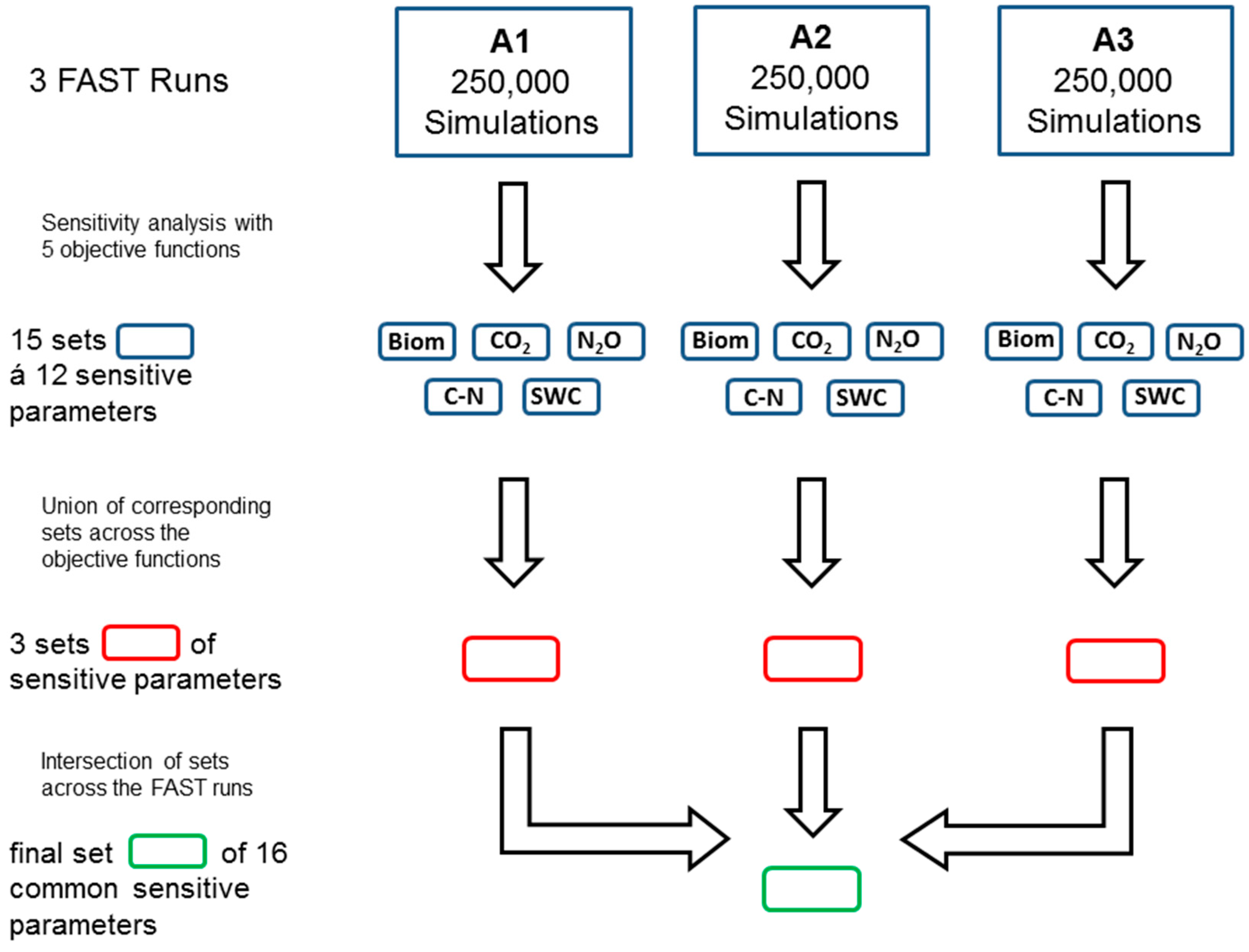
2.4. Sensitivity Analysis and Calibration

The LandscapeDNDC setup we used contains a subset of more than 100 indefinite parameters, i.e., parameters whose values are uncertain within limits chosen by expert knowledge and literature. For these parameters, a set of values had to be estimated to give the best possible agreement between simulation and measurement data under aCO₂. In this context, aCO₂ measurement data were used exclusively for calibration, while validation was based only on eCO₂ data. The agreement was quantified by using Root Mean Squared Error (RMSE) as a target function.

As the number of necessary model runs grows exponentially with the number of parameters, a sensitivity analysis was performed at the beginning to reduce the number of parameters to the most sensitive. We used the Fourier Amplitude Sensitivity Test (FAST, see [39,40]) to determine the most sensitive parameters under aCO₂ conditions on the basis of 250,000 simulations each (for details, see Figure A1 and

Table A2. Most sensitive LandscapeDNDC parameters. From left: parameters associated module, internal LandscapeDNDC parameter name, initial value, lower and upper limits of the parameter range, process-related description.

Module	Name	Int	Min	Max	Description
PLAMOX	AEJM	46,270	37,000	86,900	Activation energy for electron transport (J mol−1)
PLAMOX	AEVO	37,530	37,530	60,110	Activation energy for RubP oxygenation (J mol−1)
PLAMOX	GSMIN	21.9	5.0	60.0	Minimum stomata conductivity (mmol H2O m−2 s−1)
PLAMOX	H2OREF_A	0.5	0.2	1.0	Relative available soil water content at which stomata conductance is affected
PLAMOX	H2OREF_GS	1.0	0.2	1.0	Relative available soil water content at which stomata are fully closed
PLAMOX	NFIX_RATE	2.0	0.01	5.0	Potential nitrogen fixation rate per plant dry matter tissue and day (kg N kg−1 DM d−1)
PLAMOX	N_DEF_FACTOR	1.0	0.5	3.0	Factor defines nitrogen deficiency
PLAMOX	ROOT	0.45	0.3	0.65	Plant root fraction
PLAMOX	SLAMAX	15.0	13.0	25.0	Specific leaf area in the shade (m2 kg−1)
PLAMOX	SLAMIN	15.0	10.0	25.0	Specific leaf area in under full light (m2 kg−1)
PLAMOX	SLOPE_GSA	10.4	4.0	12.0	Slope of foliage conductivity in response to assimilation in BERRY-BALL model
site	sks_upper	1.0	0.357	3.57	Saturated hydraulic conductivity for the uppermost layer
site	vangenuchten_n_upper	1.1	1.1	1.2	VanGenuchten parameter n (uppermost layer)
METRX	METRX_F_DECOMP_T_EXP_1	2	0.5	5	Factor for temperature dependency of decomposition
METRX	METRX_KF_NIT_N2O	0.003	0.001	0.2	Maximum fraction of nitrified NH4 that goes to N2O
METRX	METRX_MIC_EFF	0.848	0.1	2	Microbial carbon use efficiency

).

For the remaining sensitive parameters (n = 16), 250,000 parameter sets for A1, A2, and A3 were calculated and simulated again using Latin Hypercube Sampling (LHS, see [41]), while all other parameters were left at their initial values. From the simulations generated by LHS, a selection of the “best” (which we call behavioral from here on) simulations based on General Likelihood Uncertainty Estimation (GLUE, see [42]) was made. GLUE allows the calibration of LandscapeDNDC to an ensemble of suitable (that is, behavioral) simulations that meet previously defined threshold objective function criteria (see Houska et al. [24]). These thresholds were chosen as upper limits for the RMSE of the behavioral simulations, meaning that each behavioral simulation must have an RMSE for each target variable less than or equal to the set value. Starting with the values by Houska et al., a further lowering was carried out, during which the subsequent threshold values (

Table 1. Maximum acceptable Root Mean Squared Error (RMSE) for the target variables during model calibration.

Target Variables	Threshold	Unit	Evaluated for Plots
Plant Biomass	1300	kg DW ha−1	A1, A2, A3
C–N ratio	4.10	-
CO2 emissions	200	mg CO2 m−2 h−1
N2O emissions	26.0	µg N2O-N m−2 h−1
Soil Water Content (SWC)	9.0	vol.-%

) were determined by simultaneous manual adjustment at all target variables and aCO₂ plots.

These simulations selected as behavioral under aCO₂ were then repeated for validation under eCO₂ while retaining the associated parameter sets. Only the input values for atmospheric CO₂ concentrations and soil properties were replaced by the measured values of the eCO₂ plots. The free open source software SPOTPY (Statistical Parameter Optimization Tool for Python, [43]) was used for all sensitivity analyses and calibration runs.

2.5. Evaluation

For the assessment of the CO₂ effect in the ensemble simulations, it had to be determined to what extent such an effect could also be proven in observation data. Statistical tests were performed to determine whether significant differences between aCO₂ and eCO₂ were present in the respective measurement data. Since the measurements were not normally distributed, we chose the nonparametric Mann–Whitney U-test to assess the probability of whether the data from aCO₂ and eCO₂ plots could belong to the same distribution.

The model ensembles of the behavioral simulations both for aCO₂ and eCO₂ were summarized as cumulative diagrams (except SWC) and compared with the measured data. The ensemble simulations were aggregated into confidence intervals with a confidence coefficient of 95%. For a better quantitative evaluation, the RMSE values of the behavioral (non-cumulative) simulations for aCO₂ and eCO₂ (see

Table A3. Average RMSE of the behavioral simulation runs.

Target Value	A1	E1	A2	E2	A3	E3
Biomass (kg DW ha−1)	1056	1242	1017	1076	1114	1010
CO2 (mg CO2 m−2 h−1)	199.3	238.9	206.0	208.8	212.22	231.6
N2O (µg N2O-N m−2 h−1)	23.85	69.12	25.71	32.83	21.71	34.00
SWC (%)	6.90	6.65	7.61	6.76	6.83	6.26

) were averaged and compared. Non-cumulative measured data were used for statistical significance tests (see

Table A4. p-Values (Mann-Whitney U Test) of aCO₂/eCO₂ measurements.

Target Value	A1/E1	A2/E2	A3/E3
Biomass	0.0433	0.431	0.110
CO2 emissions	3.992 × 10−9	0.0692	0.000293
N2O emissions	8.946 × 10−48	0.00240	1.536 × 10−22
SWC	1.255 × 10−32	2.671 × 10−8	0.00138

) and assessed on a significance level of α = 0.05.

3. Results

We evaluated the target variables of plant biomass, SWC, CO₂, and N₂O emissions. The plant C/N ratio was only used for calibration and is therefore not evaluated in detail here. Average values of the simulated C/N ratios were between 24.7 and 27.6, which is about the same range as the average measured values (25.0–28.3).

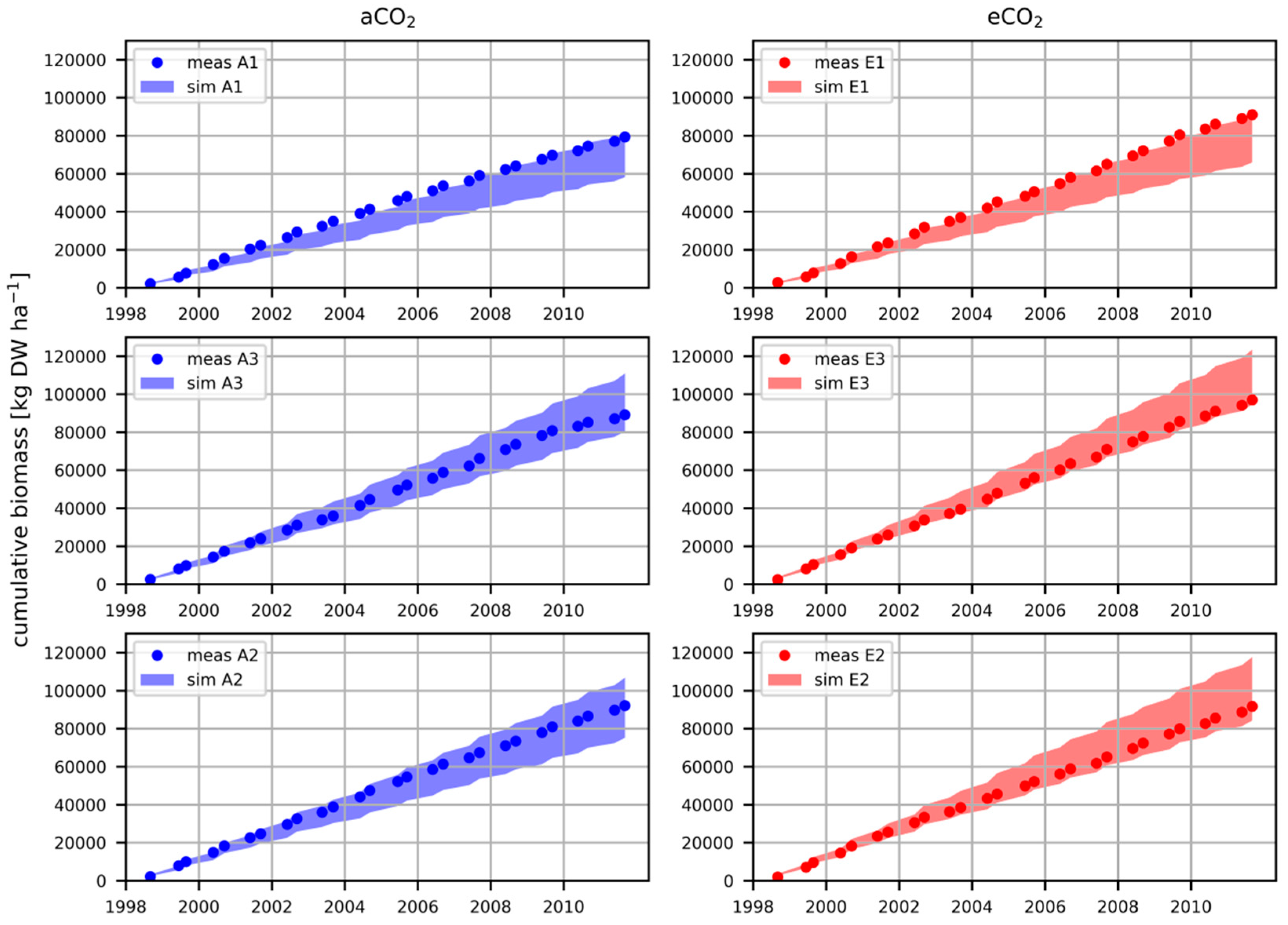
3.1. Cumulative Plant Biomass

Limits of the confidence intervals increased from aCO₂ to eCO₂ for all blocks, including almost all (96%) cumulative measured biomass values for A2, E2, A3, and E3 (Figure 1). However, significantly increased biomass due to eCO₂ was only measured for the driest block (A1/E1, see Table A4 and

Table A5. Measurement averages and number of measured data points per plot.

Target Value	A1	E1	A2	E2	A3	E3	Data Points
Biomass (kg DW ha−1)	2940	3373	3411	3400	3302	3593	27
CO2 (mg CO2 m−2 h−1)	384.8	462.1	393.5	407.3	358.8	415.1	966
N2O (µg N2O-N m−2 h−1)	8.80	32.25	10.42	13.02	9.48	16.25	1077
SWC (%)	34.8	38.4	44.4	42.1	38.4	39.5	2034

) but not for the wetter blocks (A2/E2 and A3/E3). For block A1/E1, percentage of cumulative measured values within the confidence intervals remained stable (37%/41%), even though average RMSE increased moderately (+18%, Table A3) under eCO₂. Since all measured values of A1 and E1 were close to the upper edge of their respective confidence intervals, a slight underestimation by the simulations remained at this block both for aCO₂ and eCO₂.

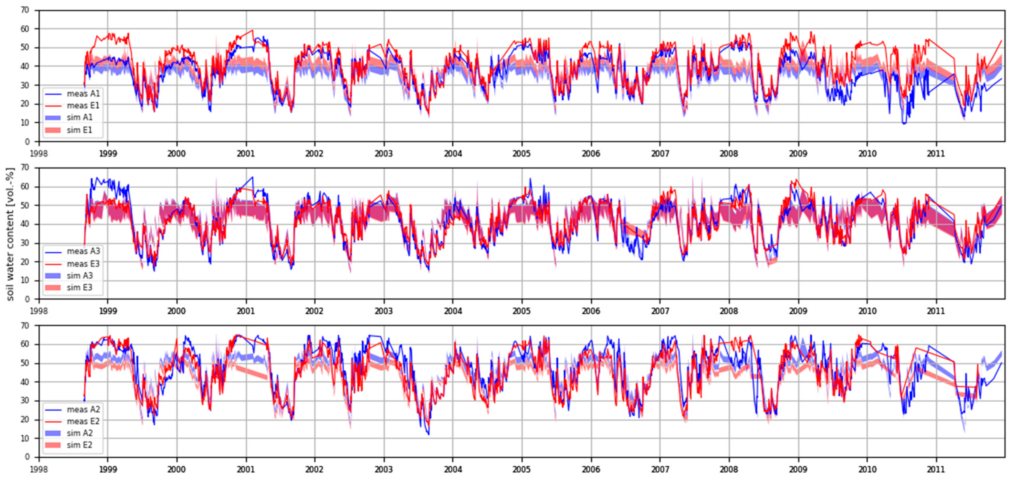
3.2. Soil Water Content

The simulations generally followed the dynamics of the observations, though the confidence intervals did not include the majority of the measured SWC values (see Figure 2). Short-term fluctuations of the SWC as well as drying phases were well captured by the simulations. Longer periods in which the soil was saturated were primarily seen in the winter months. This occurred in the simulations as well as in the measurements but at a higher level for the latter, which is why peak values of the SWC in these periods were often underestimated. This applied to both aCO₂ and eCO₂, even though the measurement curves diverged strongly in some cases, with SWC being up to twice as high under eCO₂ as under aCO₂.

The reaction of the measured SWC to elevated CO₂ varied between the plots; based on average values, the SWC increased significantly (Table A4 and Table A5) under eCO₂ at A1/E1 (+3.6 vol.-%, on average) and at A3/E3 (+1.1 vol.-%). However, at block A2/E2, SWC also decreased significantly under eCO₂ (−2.3 vol.-%). Confidence intervals showed a qualitatively similar eCO₂ reaction as the simulated SWC increased from A1 to E1 but decreased from A2 to E2. Furthermore, average RMSE (Table A3) was consistently lower during validation (E1–E3) than during calibration (A1–A3).

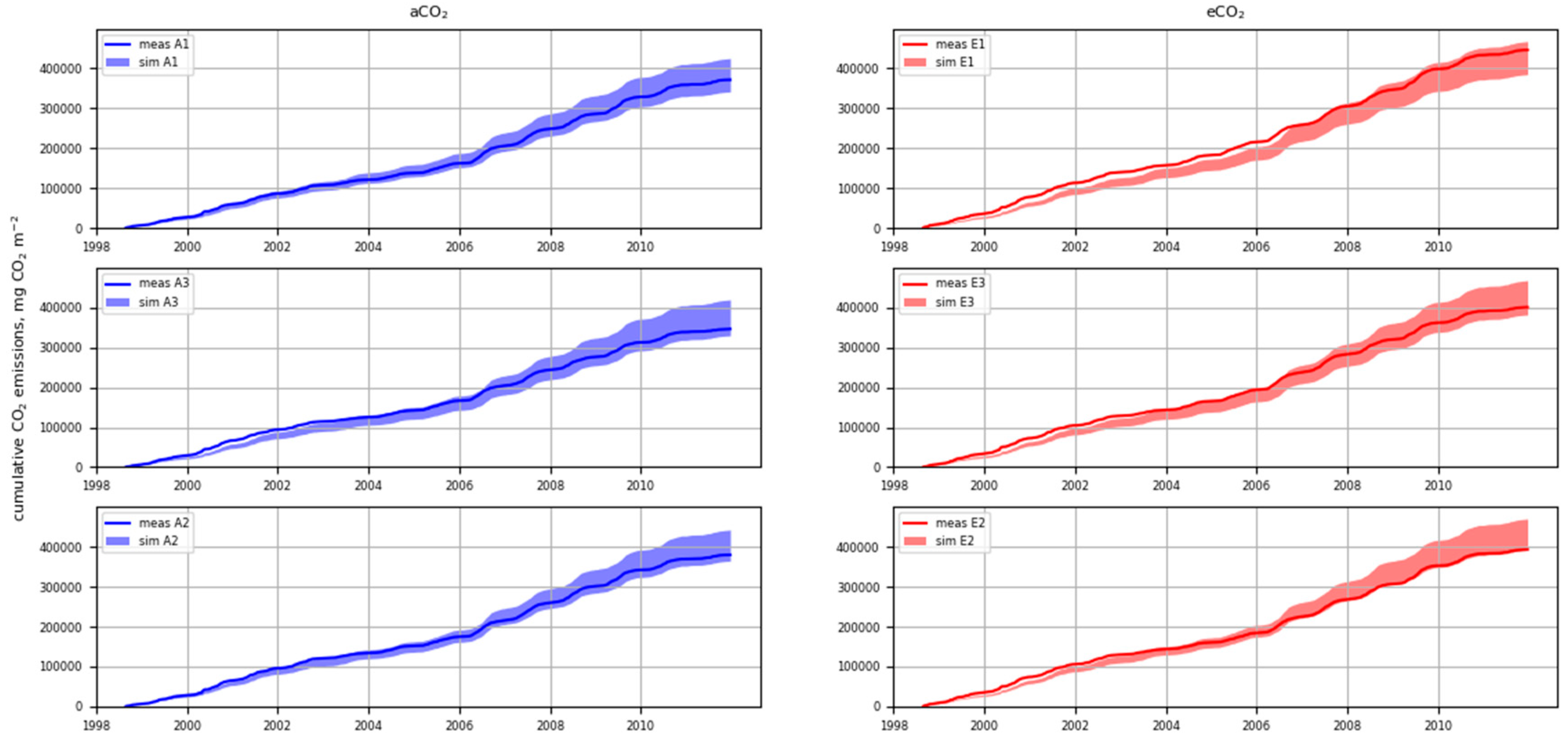
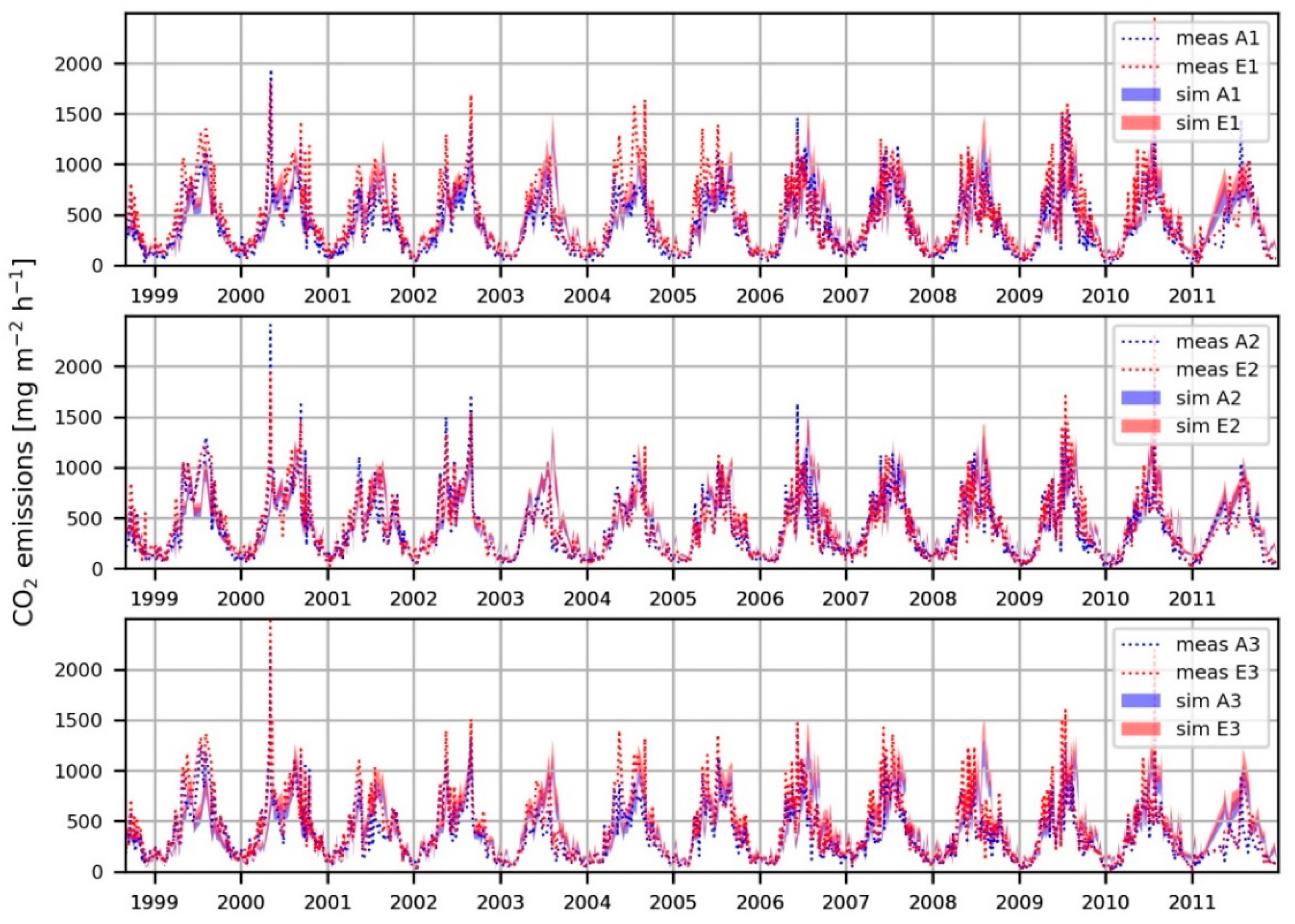
3.3. Cumulative CO₂ Emissions

As can be seen in Figure 3, measured and simulated CO₂ emissions were higher in all blocks under eCO₂ than under aCO₂. The increase was significant for A1/E1 and A3/E3 but not for A2/E2 (Table A4 and Table A5). Confidence intervals included fewer cumulative measured values under eCO₂ than under aCO₂ treatment. The proportions ranged from 94% to 44% at block A1/E1, from 79% to 65% at A2/E2, and from 70% to 69% at A3/E3. Outliers almost exclusively occurred before 2004, with the exception of E1, where the confidence interval was below the measurements until 2007. For both aCO₂ and eCO₂, all outliers were close to the upper edge of the confidence range, indicating an underestimation of LandscapeDNDC during the first half of the simulation period. No deviations occurred after 2007. Average RMSE values increased under eCO₂, with a moderate increase from A1 to E1 (about 20%) and a slight increase from A3 to E3 (about 9%). However, RMSE (Table A3) at E2 remained virtually unchanged compared to A2 (increase of about 1%).

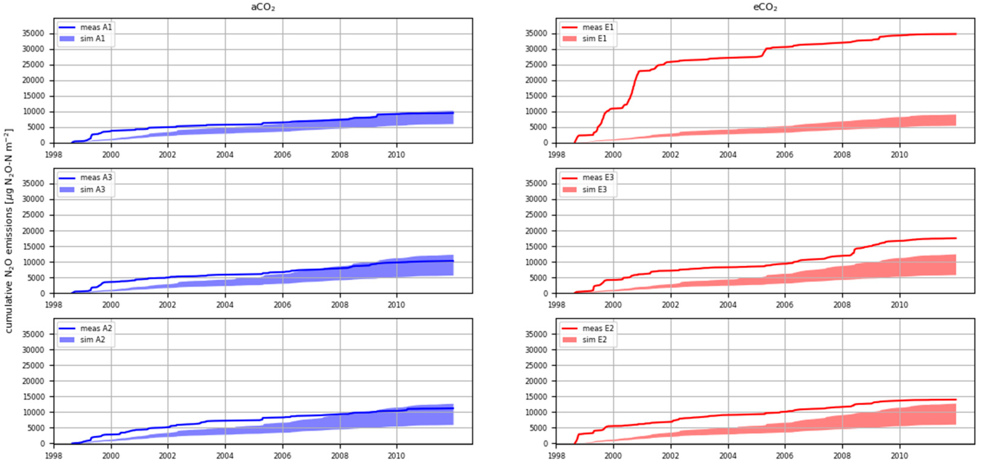
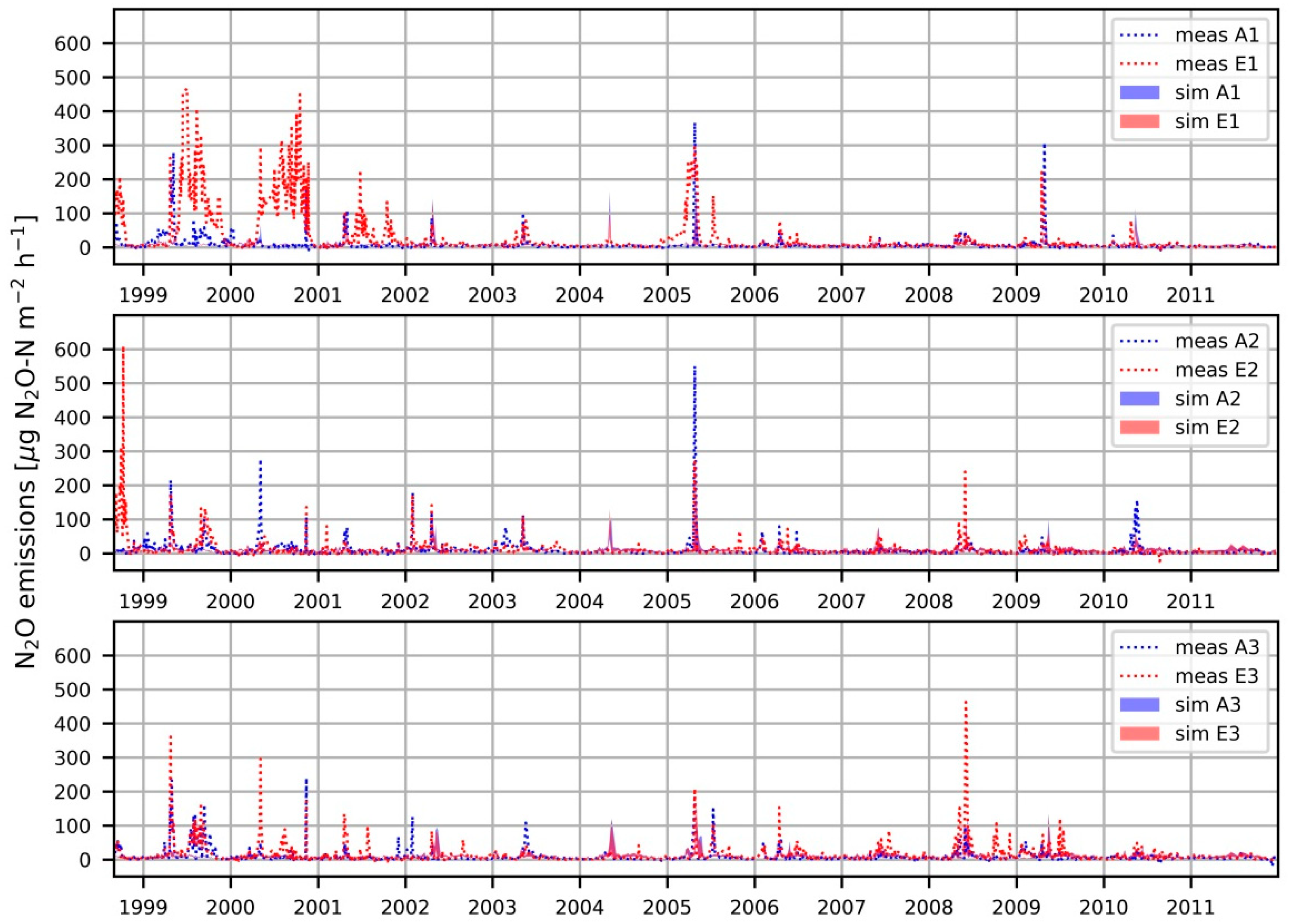
3.4. Cumulative N₂O Emissions

The measured N₂O emissions for eCO₂ increased significantly compared to aCO₂ at all blocks (Table A4), while the associated confidence intervals of the LandscapeDNDC simulations remained largely unchanged (Figure 4). For aCO₂ plots, confidence intervals included 39.2% (A1), 27.8% (A2), and 38.3% (A3) of the cumulative measured N₂O emissions, thereby underestimating the measurements, especially in the early years up to 2007/08. A very contrasting picture appeared for eCO₂, where confidence intervals were completely underestimating measurements, including none of the cumulative measured values for E1, E2, and E3. The extent of the underestimation depended strongly on the plot under consideration. If we compared the last cumulative values of measurements and the upper limit of the confidence intervals, we found a relative deviation of only 9% for E2 but of 282% for E1. For E1 in particular, a sequence of several sudden increases in cumulative N₂O emissions in the years 1998–2001 could be observed. Consequently, the RMSE (Table A3) of N₂O emissions increased for all eCO₂ plots but much more for E1 (+190% compared to A1) than for E2 (+28%) and E3 (+57%).

4. Discussion

The study presented here aimed at simulating long-term effects of atmospheric CO₂ enrichment on various environmental target variables of a grassland ecosystem. The CO₂ fumigation was performed as part of a long-term FACE experiment, from which the measured data of plant biomass, SWC, CO₂, and N₂O emissions collected continuously for more than 13 years were taken and used for calibration and validation. With the exception of N₂O emissions, it was possible to satisfactorily simulate the long-term effects of the CO₂ enrichment for all target variables.

4.1. Biomass

Agreement between simulation and measurement of biomass, especially with regard to the eCO₂ effect, varied depending on the location. For block A1/E1, agreement with measured values remained essentially the same, suggesting that the eCO₂-induced increase in biomass production was correctly simulated by the model, although biomass production itself was slightly underestimated. The opposite was observed for A2/E2, where the agreement between confidence intervals and measured values was almost perfect for both A2 and E2, although the simulations showed an increase due to elevated CO not given by the data. In context, this indicated (at least) two growth factors that were not correctly captured in the LandscapeDNDC setup used. One of these factors strengthened the CO₂-independent growth for A1/E1, while the other factor negated the CO₂ growth effect for A2/E2.

The eCO₂ reaction of the biomass differentiated according to the blocks could thus be assumed to be closely related to the respective soil hydrological conditions, which were very different for A1/E1 and A2/E2 with regard to both the mean groundwater levels and the SWC values. Previous research by Andresen et al. [44] found significant correlations of biomass with respect to CO₂ treatment and SWC on this study site, explicitly leaving open whether, in this case, a higher biomass was caused by higher SWC or vice versa. Kellner et al. [25] used a coupled hydrological plant model with physics-based soil hydraulics and performed multivariate simulations over the same period as this study. They obtained a RMSE of 1400–1500 kg DM ha⁻¹ (dry matter per hectare), which is higher than the corresponding RMSE values in this study (1000–1250 kg DM ha⁻¹). We argue that this was due to a major difference in the model setups, since Kellner et al. did not incorporate a possible N limitation for plant growth. This assumption is backed up by a previous study using an N-limited model approach, which found a massive drop in simulated biomass production if N uptake from the groundwater was ignored [26]. The same process of N uptake was also used in this study, showing that biomass production at the field site depends on groundwater-borne N supply, reflecting more N limited conditions at the driest block A1/E1 compared to the wettest block A2/E2.

4.2. SWC

Agreement between SWC simulations and measurements was satisfactory in terms of RMSE (6.2–7.6%), which is comparable to results by Kellner et al. [25] who achieved an RMSE of 6–10% using a physically-based hydrological modeling framework for the same period and field site. The confidence intervals of the simulations did not capture most of the observations but were much narrower than the fluctuation range of the measurement data. Furthermore, simulated SWC values followed the dynamic development of the observed SWC for both the annual cycle and most of the short term fluctuations. The recurrent underestimation of observed SWC peaks in winter was presumably due to the lower saturation level in the simulations, although it is not possible to clearly state to what extent this was due to the model setup or measurement errors (e.g., measured SWC values were partly higher than the pore volume and had to be cut off). Despite this, simulations captured the mean effect of CO₂ fumigation and were qualitatively correct at all blocks, even though measured SWC at A1/E1 and A2/E2 showed opposite eCO₂ reactions, while at A3/E3, almost no change occurred on average.

The reason that the eCO₂ effect turned from an increase at the driest plot E1 to a decrease at the wettest plot E2 could have been the more frequent exceedances of field capacity at E2. Niklaus et al. [45] found a similar increase of the SWC under elevated CO₂ in a grassland experiment until the effect was reversed when the field capacity was exceeded. Qi et al. [46] reported reduced transpiration and increased SWC in both simulations and observations when investigating the effect of eCO₂ on a semi-arid rangeland.

4.3. Cumulative CO₂ Emissions

The confidence intervals of the simulated cumulative CO₂ emissions generally covered the measured values well (RMSE of 199–239 mg CO₂ m⁻² h⁻¹). Only in the first years, the measured CO₂ emissions were partially underestimated, especially under eCO₂. Since the difference between measured data and simulations built up, especially in the years 1998–2001, we suspected an initial adaptation effect to CO₂ fumigation as a possible cause. This agrees with results reported by Kammann [47], who showed that there was an increase in ecosystem respiration in the first two years under eCO₂ but that it declined again in the third year. Kammann deduced that a likely cause of increased respiration was either increased rhizodeposition or increased fine root turnover.

However, even long after the initialization of the experiment (e.g., in summer 2010), emission peaks occurred that were underestimated by simulations (see Figure A2), indicating that acclimatization to eCO₂ is an ongoing process and single weather events, e.g., drying and rewetting, can mask the CO₂ effect [48].

4.4. Cumulative N₂O Emissions

The underestimation of the observed N₂O emissions by the simulation suggested that essential processes of N₂O formation were not correctly mapped in the model setup used. The regular underestimation of the SWC in winter, for example, could have led to an underestimation of anaerobic denitrification. However, since almost all N₂O peaks occurred at times outside winter when SWC was not underestimated, shortcomings in peak SWC simulation could not be mainly responsible for the underestimation of N₂O emissions (see Figure 2 and Figure A3). This would be consistent with the previous assumption that saturated soil conditions are present in periods of high SWC, leading to complete anaerobic denitrification to N₂ instead of N₂O. N₂O emission peaks during periods of lower SWC that may still arise from denitrification but do not necessarily require anaerobic conditions in the GiFACE meadow soil [49]. In principle, there is also the possibility that N₂O emissions resulted from the time-delayed aerobic denitrification of NO₃, which reached the root zone as a result of high groundwater levels or capillary rise.

Since N₂O emissions were highest under eCO₂ at the driest A1 plot, the question arises as to why aerobic denitrification was strongest at the plot with the lowest presumed NO₃ supply. An explanation could be that increased N₂O emissions arose from nitrite (NO₂⁻), as suggested by a recently published study by Moser et al. [50] on the field site. Moser et al. conducted a ¹⁵N tracing experiment, suggesting that about 90% of the additional N₂O emitted under eCO₂ originates from soil organic N, which is first oxidized to NO₂⁻ and subsequently reduced to N₂O. The trigger for this could be a priming effect that, in the early years of CO₂ fumigation, resulted in increased turnover of soil organic matter (SOM). Root exudation [50] and fine root degradation [51] were already assumed as organic N sources for increased N₂O emissions under eCO₂ and are possibly related to increased turnover processes due to fungal activity [31,51,52,53].

It should be noted that neither priming effects nor fungal decomposition processes or even oxidation of organic N are currently implemented in LandscapeDNDC. If one or more of these processes is substantially involved in N₂O production in GiFACE, this could explain the underestimation of N₂O emissions under eCO₂.

5. Conclusions

The simulations under aCO₂ showed a satisfactory agreement with measurements for all target variables, while under eCO₂, this could be achieved for biomass, SWC, and CO₂ emissions but not for N₂O emissions. The underlying problem is that N₂O emissions result from a large number of processes and factors that cannot be monitored at the ecosystem level or only for very short time frames. The consequence of this is that N₂O emission peaks are often the result of several possible causes, not all of which are necessarily known. In our case, conclusions can be drawn from the interplay of earlier investigations, long-term measurements, and simulations.

The increase in harvest biomass and CO₂ emissions under eCO₂ speaks for increased production of SOM and soil respiration. Although the increase in respiration could be attributed in part to the increased SWC under eCO₂, this did not apply to A2/E2. Here, emissions increased for both CO₂ and N₂O despite generally lower SWC at E2. This suggests that the measured increase in greenhouse gas emissions was largely due to the oxidation of SOM. If this was the case, it can be assumed that NO₃ from groundwater is also a rather indirect contributor to the increase in N₂O emissions. N₂O production could thus be explained less by anaerobic denitrification of (groundwater) NO₃ than by oxidation of labile SOM, the formation of which is forced by the combination of increased CO₂ and groundwater NO₃. Since LandscapeDNDC is currently unable to capture this, and the simulation quality of the N₂O emissions under eCO₂ differs radically from that of the other target variables, we consider the above explanation approach to be promising.

The example of N₂O emissions shows that the assessment of the complex impacts of increased CO₂ benefits from the inclusion of several interrelated environmental variables. However, this also implies that weak points in the simulation, e.g., peak SWC values, can impair the simulation quality of the other target variables and must be catered to. For the further use of LandscapeDNDC in groundwater-impacted meadows, we therefore recommend the oxidation of labile organic N to be included in the next model setup. The same applies to a better implementation of the special hydrological conditions in GiFACE. In this regard, we also recommend further studies on the influence of long-term changes in groundwater levels and nitrate concentrations in groundwater. Finally, research on the mineralization of organic material by mycorrhiza could help to improve projections about greenhouse gas emissions for grasslands under future atmospheric CO₂ conditions.

References

1. World Meteorological Organization. The State of Greenhouse Gases in the Atmosphere Based on Global Observations through 2017; WMO: Geneva, Switzerland, 2018. [Google Scholar]
2. Reichstein, M.; Bahn, M.; Ciais, P.; Frank, D.; Mahecha, M.D.; Seneviratne, S.I.; Zscheischler, J.; Beer, C.; Buchmann, N.; Frank, D.C.; et al. Climate extremes and the carbon cycle. Nature 2013, 500, 287–295. [Google Scholar] [CrossRef] [PubMed]
3. Weigel, H.-J.; Manderscheid, R. Crop growth responses to free air CO2 enrichment and nitrogen fertilization: Rotating barley, ryegrass, sugar beet and wheat. Eur. J. Agron. 2012, 43, 97–107. [Google Scholar] [CrossRef]
4. Bindi, M.; Fibbi, L.; Miglietta, F. Free Air CO2 Enrichment (FACE) of grapevine (Vitis vinifera L.): II. Growth and quality of grape and wine in response to elevated CO2 concentrations. Eur. J. Agron. 2001, 14, 145–155. [Google Scholar] [CrossRef]
5. Zak, D.R.; Holmes, W.E.; Finzi, A.C.; Norby, R.J.; Schlesinger, W.H. Soil Nitrogen Cycling Under Elevated Co2: A Synthesis of Forest Face Experiments. Ecol. Appl. 2003, 13, 1508–1514. [Google Scholar] [CrossRef] [Green Version]
6. Luo, Y.; Su, B.; Currie, W.S.; Dukes, J.S.; Finzi, A.C.; Hartwig, U.; Hungate, B.; McMurtrie, R.E.; Oren, R.; Parton, W.J.; et al. Progressive nitrogen limitation of ecosystem responses to rising atmospheric carbon dioxide. Bioscience 2004, 54, 731–739. [Google Scholar] [CrossRef] [Green Version]
7. Gärdenäs, A.I.; Ågren, G.I.; Bird, J.A.; Clarholm, M.; Hallin, S.; Ineson, P.; Kätterer, T.; Knicker, H.; Nilsson, S.I.; Näsholm, T.; et al. Knowledge gaps in soil carbon and nitrogen interactions—From molecular to global scale. Soil Biol. Biochem. 2011, 43, 702–717. [Google Scholar] [CrossRef]
8. Feng, Z.; Rütting, T.; Pleijel, H.; Wallin, G.; Reich, P.B.; Kammann, C.I.; Newton, P.C.D.; Kobayashi, K.; Luo, Y.; Uddling, J. Constraints to nitrogen acquisition of terrestrial plants under elevated CO2. Glob. Chang. Biol. 2015, 21, 3152–3168. [Google Scholar] [CrossRef]
9. Van Groenigen, K.J.; Qi, X.; Osenberg, C.W.; Luo, Y.; Hungate, B.A. Faster Decomposition Under Increased Atmospheric CO2 Limits Soil Carbon Storage. Science 2014, 344, 508–509. [Google Scholar] [CrossRef]
10. Cheng, W.; Johnson, D.W. Elevated CO2, rhizosphere processes, and soil organic matter decomposition. Plant Soil 1998, 202, 167–174. [Google Scholar] [CrossRef]
11. Phillips, D.A.; Fox, T.C.; Six, J. Root exudation (net efflux of amino acids) may increase rhizodeposition under elevated CO2. Glob. Chang. Biol. 2006, 12, 561–567. [Google Scholar] [CrossRef]
12. Terrer, C.; Vicca, S.; Hungate, B.A.; Phillips, R.P.; Prentice, I.C. Mycorrhizal association as a primary control of the CO2 fertilization effect. Science 2016, 353, 72–74. [Google Scholar] [CrossRef] [Green Version]
13. Müller, C.; Sherlock, R.R.; Williams, P.H. Mechanistic model for nitrous oxide emission via nitrification and denitrification. Biol. Fertil. Soils 1997, 24, 231–238. [Google Scholar] [CrossRef]
14. Ryan, M.; Müller, C.; Di, H.J.; Cameron, K.C. The use of artificial neural networks (ANNs) to simulate N2O emissions from a temperate grassland ecosystem. Ecol. Model. 2004, 175, 189–194. [Google Scholar] [CrossRef]
15. Zhang, X.; Niu, G.-Y.; Elshall, A.S.; Ye, M.; Barron-Gafford, G.A.; Pavao-Zuckerman, M. Assessing five evolving microbial enzyme models against field measurements from a semiarid savannah—What are the mechanisms of soil respiration pulses? Geophys. Res. Lett. 2014, 41, 6428–6434. [Google Scholar] [CrossRef]
16. Sitch, S.; Smith, B.; Prentice, I.C.; Arneth, A.; Bondeau, A.; Cramer, W.; Kaplan, J.O.; Levis, S.; Lucht, W.; Sykes, M.T.; et al. Evaluation of ecosystem dynamics, plant geography and terrestrial carbon cycling in the LPJ dynamic global vegetation model. Glob. Chang. Biol. 2003, 9, 161–185. [Google Scholar] [CrossRef]
17. Xu-Ri; Prentice, I.C.; Spahni, R.; Niu, H.S. Modelling terrestrial nitrous oxide emissions and implications for climate feedback. New Phytol. 2012, 196, 472–488. [Google Scholar] [CrossRef] [PubMed]
18. Cheng, L.; Zhang, L.; Wang, Y.-P.; Yu, Q.; Eamus, D. Quantifying the effects of elevated CO2 on water budgets by combining FACE data with an ecohydrological model. Ecohydrology 2014, 7, 1574–1588. [Google Scholar] [CrossRef]
19. Li, F.Y.; Newton, P.C.D.; Lieffering, M. Testing simulations of intra- and inter-annual variation in the plant production response to elevated CO2 against measurements from an 11-year FACE experiment on grazed pasture. Glob. Chang. Biol. 2014, 20, 228–239. [Google Scholar] [CrossRef]
20. De Kauwe, M.G.; Medlyn, B.E.; Zaehle, S.; Walker, A.P.; Dietze, M.C.; Wang, Y.-P.; Luo, Y.; Jain, A.K.; El-Masri, B.; Hickler, T.; et al. Where does the carbon go? A model—Data intercomparison of vegetation carbon allocation and turnover processes at two temperate forest free-air CO2 enrichment sites. New Phytol. 2014, 203, 883–899. [Google Scholar] [CrossRef] [Green Version]
21. Zaehle, S.; Medlyn, B.E.; De Kauwe, M.G.; Walker, A.P.; Dietze, M.C.; Hickler, T.; Luo, Y.; Wang, Y.-P.; El-Masri, B.; Thornton, P.; et al. Evaluation of 11 terrestrial carbon–nitrogen cycle models against observations from two temperate Free-Air CO2 Enrichment studies. New Phytol. 2014, 202, 803–822. [Google Scholar] [CrossRef] [Green Version]
22. Walker, A.P.; Hanson, P.J.; De Kauwe, M.G.; Medlyn, B.E.; Zaehle, S.; Asao, S.; Dietze, M.; Hickler, T.; Huntingford, C.; Iversen, C.M.; et al. Comprehensive ecosystem model-data synthesis using multiple data sets at two temperate forest free-air CO2 enrichment experiments: Model performance at ambient CO2 concentration. J. Geophys. Res. Biogeosci. 2014, 119, 2013JG002553. [Google Scholar] [CrossRef] [Green Version]
23. Walker, A.P.; Zaehle, S.; Medlyn, B.E.; De Kauwe, M.G.; Asao, S.; Hickler, T.; Parton, W.; Ricciuto, D.M.; Wang, Y.-P.; Wårlind, D.; et al. Predicting long-term carbon sequestration in response to CO2 enrichment: How and why do current ecosystem models differ? Glob. Biogeochem. Cycles 2015, 29, 2014GB004995. [Google Scholar] [CrossRef]
24. Houska, T.; Kraft, P.; Liebermann, R.; Klatt, S.; Kraus, D.; Haas, E.; Santabarbara, I.; Kiese, R.; Butterbach-Bahl, K.; Müller, C.; et al. Rejecting hydro-biogeochemical model structures by multi-criteria evaluation. Environ. Model. Softw. 2017, 93, 1–12. [Google Scholar] [CrossRef]
25. Kellner, J.; Multsch, S.; Houska, T.; Kraft, P.; Müller, C.; Breuer, L. A coupled hydrological-plant growth model for simulating the effect of elevated CO2 on a temperate grassland. Agric. For. Meteorol. 2017, 246, 42–50. [Google Scholar] [CrossRef]
26. Liebermann, R.; Breuer, L.; Houska, T.; Klatt, S.; Kraus, D.; Haas, E.; Müller, C.; Kraft, P. Closing the N-Budget: How Simulated Groundwater-Borne Nitrate Supply Affects Plant Growth and Greenhouse Gas Emissions on Temperate Grassland. Atmosphere 2018, 9, 407. [Google Scholar] [CrossRef] [Green Version]
27. Haas, E.; Klatt, S.; Fröhlich, A.; Kraft, P.; Werner, C.; Kiese, R.; Grote, R.; Breuer, L.; Butterbach-Bahl, K. LandscapeDNDC: A process model for simulation of biosphere–atmosphere–hydrosphere exchange processes at site and regional scale. Landsc. Ecol. 2013, 28, 615–636. [Google Scholar] [CrossRef]
28. Grünhage, L.; Schmitt, J.; Hertstein, U.; Janze, S.; Peter, M.; Jäger, H.-J., III. Beschreibung der Versuchsfläche. In Auswirkungen Dynamischer Veränderungen der Luftzusammensetzung und des Klimas auf Terrestrische Ökosysteme in Hessen-II-Umweltbeobachtungs- und Klimafolgenforschungsstation Linden, Jahresbericht 1995; Schriftenreihe der Hessischen Landesanstalt für Umwelt 220; Umweltplanung, Arbeits- und Umweltschutz: Wiesbaden, Germany, 1996; ISBN 3-89026-236-8. [Google Scholar]
29. Jäger, H.-J.; Schmidt, S.W.; Kammann, C.; Grünhage, L.; Müller, C.; Hanewald, K. The University of Giessen Free-Air Carbon dioxide Enrichment study: Description of the experimental site and of a new enrichment system. J. Appl. Bot. 2003, 77, 117–127. [Google Scholar]
30. Patterson, D.E.; Smith, M.W. The use of time domain reflectometry for the measurement of unfrozen water content in frozen soils. Cold Reg. Sci. Technol. 1980, 3, 205–210. [Google Scholar] [CrossRef]
31. Kammann, C.; Müller, C.; Grünhage, L.; Jäger, H.-J. Elevated CO2 stimulates N2O emissions in permanent grassland. Soil Biol. Biochem. 2008, 40, 2194–2205. [Google Scholar] [CrossRef]
32. Kammann, C.; Grünhage, L.; Jäger, H.-J., II. N2O- und CH4-Flüsse in der bodennahen Atmosphäre eines extensiv genutzten Grünlandökosystems. In Auswirkungen Dynamischer Veränderungen der Luftzusammensetzung und des Klimas auf Terrestrische Ökosysteme in Hessen-III-Umweltbeobachtungs- und Klimafolgenforschungsstation Linden, Berichtszeitraum 1996–1999; Schriftenreihe der Hessischen Landesanstalt für Umwelt; Umweltplanung, Arbeits- und Umweltschutz: Wiesbaden, Germany, 2000; Volume 274, ISBN 3-89026-311-9. [Google Scholar]
33. Grote, R.; Lehmann, E.; Brümmer, C.; Brüggemann, N.; Szarzynski, J.; Kunstmann, H. Modelling and observation of biosphere–atmosphere interactions in natural savannah in Burkina Faso, West Africa. Phys. Chem. Earth Parts ABC 2009, 34, 251–260. [Google Scholar] [CrossRef]
34. Grote, R.; Lavoir, A.-V.; Rambal, S.; Staudt, M.; Zimmer, I.; Schnitzler, J.-P. Modelling the drought impact on monoterpene fluxes from an evergreen Mediterranean forest canopy. Oecologia 2009, 160, 213–223. [Google Scholar] [CrossRef] [PubMed]
35. Kraus, D.; Weller, S.; Klatt, S.; Santabárbara, I.; Haas, E.; Wassmann, R.; Werner, C.; Kiese, R.; Butterbach-Bahl, K. How well can we assess impacts of agricultural land management changes on the total greenhouse gas balance (CO2, CH4 and N2O) of tropical rice-cropping systems with a biogeochemical model? Agric. Ecosyst. Environ. 2016, 224, 104–115. [Google Scholar] [CrossRef]
36. Farquhar, G.D.; von Caemmerer, S.; Berry, J.A. A biochemical model of photosynthetic CO2 assimilation in leaves of C3 species. Planta 1980, 149, 78–90. [Google Scholar] [CrossRef] [PubMed] [Green Version]
37. Kraus, D.; Weller, S.; Klatt, S.; Haas, E.; Wassmann, R.; Kiese, R.; Butterbach-Bahl, K. A new LandscapeDNDC biogeochemical module to predict CH4 and N2O emissions from lowland rice and upland cropping systems. Plant Soil 2014, 386, 125–149. [Google Scholar] [CrossRef]
38. Dirnböck, T.; Kraus, D.; Grote, R.; Klatt, S.; Kobler, J.; Schindlbacher, A.; Seidl, R.; Thom, D.; Kiese, R. Substantial understory contribution to the C sink of a European temperate mountain forest landscape. Landsc. Ecol. under review.
39. Cukier, R.I.; Fortuin, C.M.; Shuler, K.E.; Petschek, A.G.; Schaibly, J.H. Study of the sensitivity of coupled reaction systems to uncertainties in rate coefficients. I Theory. J. Chem. Phys. 1973, 59, 3873–3878. [Google Scholar] [CrossRef]
40. Saltelli, A.; Tarantola, S.; Chan, K.P.-S. A Quantitative Model-Independent Method for Global Sensitivity Analysis of Model Output. Technometrics 1999, 41, 39–56. [Google Scholar] [CrossRef]
41. McKay, M.D.; Beckman, R.J.; Conover, W.J. A Comparison of Three Methods for Selecting Values of Input Variables in the Analysis of Output from a Computer Code. Technometrics 1979, 21, 239–245. [Google Scholar]
42. Beven, K.; Freer, J. Equifinality, data assimilation, and uncertainty estimation in mechanistic modelling of complex environmental systems using the GLUE methodology. J. Hydrol. 2001, 249, 11–29. [Google Scholar] [CrossRef]
43. Houska, T.; Kraft, P.; Chamorro-Chavez, A.; Breuer, L. SPOTting Model Parameters Using a Ready-Made Python Package. PLoS ONE 2015, 10, e0145180. [Google Scholar] [CrossRef]
44. Andresen, L.C.; Yuan, N.; Seibert, R.; Moser, G.; Kammann, C.I.; Luterbacher, J.; Erbs, M.; Müller, C. Biomass responses in a temperate European grassland through 17 years of elevated CO2. Glob. Chang. Biol. 2017, 24, 3875–3885. [Google Scholar] [CrossRef] [PubMed]
45. Niklaus, P.A.; Spinnler, D.; Körner, C. Soil moisture dynamics of calcareous grassland under elevated CO2. Oecologia 1998, 117, 201–208. [Google Scholar] [CrossRef] [PubMed]
46. Qi, Z.; Morgan, J.A.; McMaster, G.S.; Ahuja, L.R.; Derner, J.D. Simulating Carbon Dioxide Effects on Range Plant Growth and Water Use with GPFARM-Range Model. Rangel. Ecol. Manag. 2015, 68, 423–431. [Google Scholar] [CrossRef]
47. Kammann, C. Die Auswirkung Steigender Atmosphärischer CO2-Konzentrationen auf die Flüsse der Klimaspurengase N2O und CH4 in Einem Grünland-Ökosystem. Available online: http://geb.uni-giessen.de/geb/volltexte/2001/491/ (accessed on 7 March 2019).
48. Xiang, S.-R.; Doyle, A.; Holden, P.A.; Schimel, J.P. Drying and rewetting effects on C and N mineralization and microbial activity in surface and subsurface California grassland soils. Soil Biol. Biochem. 2008, 40, 2281–2289. [Google Scholar] [CrossRef]
49. Müller, C.; Stevens, R.J.; Laughlin, R.J.; Jäger, H.-J. Microbial processes and the site of N2O production in a temperate grassland soil. Soil Biol. Biochem. 2004, 36, 453–461. [Google Scholar] [CrossRef]
50. Moser, G.; Gorenflo, A.; Brenzinger, K.; Keidel, L.; Braker, G.; Marhan, S.; Clough, T.J.; Müller, C. Explaining the doubling of N2O emissions under elevated CO2 in the Giessen FACE via in-field 15N tracing. Glob. Chang. Biol. 2018, 24, 3897–3910. [Google Scholar] [CrossRef]
51. Kammann, C.; Grünhage, L.; Grüters, U.; Janze, S.; Jäger, H.-J. Response of aboveground grassland biomass and soil moisture to moderate long-term CO2 enrichment. Basic Appl. Ecol. 2005, 6, 351–365. [Google Scholar] [CrossRef]
52. Denef, K.; Bubenheim, H.; Lenhart, K.; Vermeulen, J.; Van Cleemput, O.; Boeckx, P.; Müller, C. Community shifts and carbon translocation within metabolically-active rhizosphere microorganisms in grasslands under elevated CO2. Biogeosciences 2007, 4, 769–779. [Google Scholar] [CrossRef] [Green Version]
53. Guenet, B.; Lenhart, K.; Leloup, J.; Giusti-Miller, S.; Pouteau, V.; Mora, P.; Nunan, N.; Abbadie, L. The impact of long-term CO2 enrichment and moisture levels on soil microbial community structure and enzyme activities. Geoderma 2012, 170, 331–336. [Google Scholar] [CrossRef]
54. Dämmgen, U.; Grünhage, L.; Schaaf, S. The precision and spatial variability of some meteorological parameters needed to determine ver­tical fluxes of air constituents. Landbauforschung Volkenrode 2005, 55, 29–37. [Google Scholar]
55. Scholz-Seidel, C.D. UV 2 Messungen der Bulk-Depositionen sedimentierender anorganischer Spezies (September 1993 bis Dezember 1995). In Auswirkungen Dynamischer Veränderungen der Luftzusammensetzung und des Klimas auf Terrestrische Ökosysteme in Hessen-II-Umweltbeobachtungs- und Klimafolgenforschungsstation Linden, Jahresbericht 1995; Schriftenreihe der Hessischen Landesanstalt für Umwelt 220; Umweltplanung, Arbeits- und Umweltschutz: Wiesbaden, Germany, 1996. [Google Scholar]
Figure 1. Cumulative measured and simulated values of harvested plant biomass for ambient (aCO2) and elevated CO2 (eCO2) Free Air Carbon dioxide Enrichment (FACE) rings. Plots are arranged according to increasing soil moisture from driest (top, A1/E1) to medium (middle, A3/E3) and wettest (bottom, A2/E2) rings. Measurements are depicted in dots; confidence intervals of simulations are depicted as colored areas.
Agronomy 10 00050 g001
Figure 2. Time series of soil water content in 0–15 cm soil depths from ambient (aCO2) and elevated CO2 (eCO2) FACE rings. Plots are arranged according to increasing soil moisture from driest (top, A1/E1) to medium (middle, A3/E3) and wettest (bottom, A2/E2) rings. Measurements are depicted in lines, and confidence intervals of simulations are depicted as colored areas.
Agronomy 10 00050 g002
Figure 3. Cumulative measured and simulated CO2 emissions from ambient (aCO2) and elevated CO2 (eCO2) FACE rings. Plots are arranged according to increasing soil moisture from driest (top, A1/E1) to medium (middle, A3/E3) and wettest (bottom, A2/E2) rings. Measurements are depicted in lines, and confidence intervals of simulations are depicted as colored areas.
Agronomy 10 00050 g003
Figure 4. Cumulative measured and simulated N2O emissions from ambient (aCO2) and elevated CO2 (eCO2) FACE rings. Plots are arranged according to increasing soil moisture from driest (top, A1/E1) to medium (middle, A3/E3) and wettest (bottom, A2/E2) rings. Measurements are depicted in lines, and confidence intervals of simulations are depicted as colored areas.
Agronomy 10 00050 g004