


Abstract
The classical phenomenon of motion of a projectile fired (thrown) into the horizon through resistive air charging a quadratic drag onto the object is revisited in this paper. No exact solution is known that describes the full physical event under such an exerted resistance force. Finding elegant analytical approximations for the most interesting engineering features of dynamical behavior of the projectile is the principal target. Within this purpose, some analytical explicit expressions are derived that accurately predict the maximum height, its arrival time as well as the flight range of the projectile at the highest ascent. The most significant property of the proposed formulas is that they are not restricted to the initial speed and firing angle of the object, nor to the drag coefficient of the medium. In combination with the available approximations in the literature, it is possible to gain information about the flight and complete the picture of a trajectory with high precision, without having to numerically simulate the full governing equations of motion.
Export citation and abstract BibTeX RIS
1. Introduction
The two-dimensional motion of a point mass or projectile has a long history in the literature, having enumerable real life applications in science and engineering, such as bullets in ballistics [1], balls in sports [2–4] and [5], rockets in war machines [6], sand in various environments [7], particles in fluids [8], and so on. Therefore, it has been the focus of researches for a couple of centuries. Via empirical approximations of the angular function that appears in the integrand, which permit the integration to be performed analytically, we in the present paper are also interested in the dynamic behaviour of the thrown projectile into air at an initial angle with an initial speed taking into account the commonly known physical laws involving a resistance force proportional to the velocity square.
It is now well established that when an object is fired to the horizon with an initial angle and speed, it encounters a drag force due the medium [9]. When this drag is omitted or is linearly dependent on the speed of the object, exact formulas for the motion are available (see [10] and [11]). However, such a drag force is only realistic during the travel of the object in the range of low speeds pointing to small Reynolds numbers within the framework of Stokes' flow. At the times of flight when the object moves with relatively high speeds, the drag force must be replaced with a quadratic law [12]. In this situation, even though an exact solution for the tangential velocity in the direction of motion can be obtained, the time of flight and the locations of the projectile along the vertical and horizontal axes can not be exactly determined [13], requiring one to resort to the numerical simulation or analytical approximation.
Due to the difficulty in the derivation of exact trajectories, besides numerical approaches, other perturbation techniques are also possible to implement under particular restrictive cases. [12] solved the governing equations for short and large times and derived neat approximate solutions. Such an analysis was also conducted in [14] for low, high and split angle trajectory regimes, and in [15] for a low-angle trajectory. Analytic approximate solutions were also found through the homotopy analysis method in [16], but the homotopy series solutions are cumbersome and not easy to interpret.
In addition to the perturbation solutions, simple closed-form approximate empirical formulas were also proposed in several successive papers by Chudinov [13, 17–20]. These works are highly appreciated, even if the formulas are only valid for special cases, they correctly simulate the phenomenon up to a desired precision and enable one to discern the most important features of the action of the point mass. They are not only useful for specialists in the field but also for undergraduate and graduate students.
Unfortunately, both perturbation solutions and the proposed empirical equations presently existing in the open literature have low accuracy and are confined to a very limited range of physical parameters influencing the motion of a projectile. Therefore, the present motivation is to derive exact approximate solutions from a strong mathematical background. A user-friendly structure and accuracy of the presentations are also highly desirable. Approximating the corresponding integrals with proper functions permitting the integration to be performed analytically, the maximum height, the arrival time of descent and the horizontal distance of the projectile at the maximum vertical distance are presented through elegant explicit formulas. These are valid for the initial speed, initial angle and quadratic drag force coefficient. When combined with the equations of Chudinov [13, 17–20], it is now possible to accurately predict the significant flow conditions and to simulate the motion of a trajectory without having to employ any numerical scheme. These formulas are also beneficial to specialists actively working in the field as well as undergraduate and graduate students of engineering.
2. Physical background and the model
Although the governing equations can be found in many sources, some of which are already cited here, for a complete description of the physical phenomenon, we briefly outline the derivation of them in what follows. Let us consider the motion of a point mass m or projectile launched at an angle  with an initial speed V0 encountering a quadratic resistance force
  . A simple sketch of the physical event is displayed in figure 1. It is assumed that the projectile is at the initial instant standing at the origin. Here g is the acceleration of gravity, k0 is the drag constant and V is the speed of the object in the tangential direction. At any angle θ (or time t), the equations of motion along the tangential direction due to Newton's second law and the principal normal direction due to the centrifugal law are written as


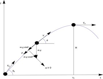
Figure 1. Basic model representing the physics of a moving projectile.
Download figure:
Standard image High-resolution imageThe horizontal and vertical distances (x, y) are related to the motion of the projectile via the kinematic relations

A more convenient non-dimensional form of equations (1)–(3) can be achieved after the transformations

that yields


with  standing for the dimensionless drag coefficient. It appears that the motion is only implicitly affected by the initial velocity after defining the parameter p. Hence, we have two fundamental parameters; namely
  and p, for a description of the complete picture of motion.
The practical physical quantities of concern in the present analysis are

representing the the maximum height of the projectile, the highest ascent time and the abscissa of the trajectory apex, respectively.
3. Explicit approximations
As mentioned before, for small  or small p or small U, explicit approximations are already available in the literature. Our objective is to extract explicit analytic estimates without any limitation on the parameters
  and p.
Solving (5) results in the exact solution for the speed of the object

However, no exact solutions for the dimensionless time τ or for the position (X,Y) can be found by a direct integration of (6) and (7), since the integrals

seem impossible to evaluate in terms of the standard or advanced functions of mathematics.
A close inspection proves that equations in (10) are not exactly integrable owing to the complicated nature of  running from
  to
to  within the scaled speed U. A good approximation, on the other hand, of the physical phenomenon highly relies upon how well the function
  is estimated. Even though, over the whole region of physical interest, it seems hard, the best possible approximating function of
  (that makes (10) exactly integrable) over the shorter interval
 ![$[0,{\theta }_{0}]$](https://content.cld.iop.org/journals/0143-0807/37/3/035001/revision1/ejpaa1c56ieqn12.gif) can be accomplished via the interpolating function
can be accomplished via the interpolating function

where α and β can be determined in such a way so as to connect fa to f smoothly

The equations in (12) are necessary since  varies faster near
  , rather than
  where the upward motion ends. Consequently, it is found from (12)
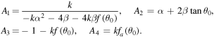
By virtue of (13), the equations in (10) are now exactly integrable, leading to good approximations for the maximum height of ascent, the abscissa of maximum ascent and the time of maximum ascent, respectively, in the forms
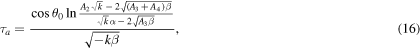
where  and
and
Combining (14)–(16) with the formulas in Chudinov's papers enables us to estimate the most important factors in projectile motion as well as the trajectory of the projectile with an adequate accuracy, without any limitation on the throwing angle, throwing speed and drag coefficient of the quadratic resistance law. Specifically, as described in Chudinov's papers [13, 17–20], the realized motion time T, the velocity at the trajectory apex  , the flight range L, the impact angle with respect to the horizontal
  and the final velocity V1, which are of utmost physical and practical interest, can be identified, as will be discussed in the coming section.
4. Results and discussions
Let us first justify the accuracy of the approximations derived in (14)–(16). To this end, the following limiting values can be calculated from (14) to (16)


These are the well-known data from the classical analysis; (17) and (18) correspond to the vacuum and infinite air resistance cases, (19) is associated with the free downward falling and (20) represents the traditional one-dimensional upward throwing mechanical problem.
In addition to this, the motion of a baseball with the conditions  , p = 1 and g=9.81 are compared in table 1 with the proposed formulae in Chudinov [13] as well as with the exact numerical integration. It is evident how good the mechanical properties of the point mass are predicted via the formulas (14)–(16). Table 1 is also a clear indicator that the simple formulas in Chudinov [13] are better be replaced with the present ones, particularly for a good estimate for the maximum ascent time.
Table 1. Comparison of a baseball problem with Chudinov [13] and exact numerical integration.
| Numerical | Chudinov | Present | |
|---|---|---|---|
| H | 0.182764 | 0.184699 | 0.182090 |
| Xa | 0.325102 | 0.329128 | 0.323581 |

|
0.566820 | 0.607753 | 0.565427 |
It is, moreover, compared the exact speed of the projectile (9) with the approximate correspondence under (11) in the particular domain ![$[0,{\theta }_{0}]$](https://content.cld.iop.org/journals/0143-0807/37/3/035001/revision1/ejpaa1c56ieqn21.gif) . Figures 2(a)-(d) demonstrate the absolute errors with p = 1 at different starting angles
. Figures 2(a)-(d) demonstrate the absolute errors with p = 1 at different starting angles  . The absolute errors falling below 0.3% are clear evidence for the accuracy of the proposed formulas in the present study.

Figure 2. Absolute errors in U between the exact and present approximation with p = 1. (a)  , (b)
, (b)  , (c)
, (c)  and (d)
Download figure:
Standard image High-resolution imageHaving anticipated the advantages of the presented formulas in (14)–(16), it is now time to fully exploit the gains from them. The physical expectations for the maximum height, the time of ascent and the abscissa of ascent with respect to the initial angle as well as to the drag coefficient are exhibited to be satisfactorily met from figures 3(a)-(c).

Figure 3. Variation of extremum values versus  . (a) H, (b) Xa and (c)
  .
.
Download figure:
Standard image High-resolution imageAs also stated in Chudinov [13], the most important parameter to know as a priority is the maximum height H, since it is possible to relate the other mechanical features to this parameter through simple empirical relations. As a result, we may associate the present more realistic H in (14) with the formulae presented in Chudinov [13]; namely, at a prescribed  and p, the motion time
  , the velocity at the trajectory apex
  (exact), the flight range
  , the impact angle with respect to the horizontal
 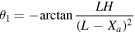 and the final velocity
  . Combining our value of H with these, table 2 lists such engineering quantities at various p for the chosen angle
  . It is apparent that Chudinov's results are deviating from the numerical results for increasing p, whereas our results are in full agreement with those from the numerics.
Table 2.
Comparison of a baseball problem; exact numerical integration (first column), Chudinov (second column) and present (third column) at  .
.
| p = 0.1 | p = 1 | p = 10 | |||||||
|---|---|---|---|---|---|---|---|---|---|
| H | 0.24009 | 0.24146 | 0.23994 | 0.18276 | 0.18470 | 0.18209 | 0.07003 | 0.05512 | 0.06957 |
| Xa | 0.47173 | 0.47408 | 0.47135 | 0.32510 | 0.32913 | 0.32358 | 0.10197 | 0.08560 | 0.10112 |

|
0.68674 | 0.69488 | 0.68646 | 0.56682 | 0.60775 | 0.56543 | 0.30102 | 0.33202 | 0.29950 |
| T | 1.38575 | 1.38986 | 1.38546 | 1.20474 | 1.21556 | 1.20695 | 0.73487 | 0.66405 | 0.74604 |
| L | 0.92838 | 0.93081 | 0.92787 | 0.58902 | 0.58650 | 0.58234 | 0.15957 | 0.13293 | 0.14934 |

|
−0.8193 | -0.8227 | −0.8184 | -0.9996 | −1.0220 | -1.0076 | −1.2947 | -1.2741 | -1.3007 |
| U1 | 0.93023 | 0.93318 | 0.92941 | 0.63823 | 0.64996 | 0.64235 | 0.27795 | 0.27399 | 0.28869 |
It is also possible to get more accurate trajectories from the given formula in Chudinov [13];
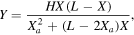
thanks to the present approximation for H in (14). Indeed, figures 4(a)–(c) validate the present model, particularly over ![$X\in [0,{X}_{a}]$](https://content.cld.iop.org/journals/0143-0807/37/3/035001/revision1/ejpaa1c56ieqn39.gif) for the entire drag coefficient p.
for the entire drag coefficient p.

Figure 4. Trajectories; continuous lines from Chudinov, dotted lines from the present and dashed lines from the numerical integration. (a) p = 0.1, (b) p = 1 and (c) p = 10.
Download figure:
Standard image High-resolution imageThe shortcomings for the trajectories in figures 4(a)–(c) specifically occurring after the peak location can be overcome by estimating the speed V over the whole physical interval ![$\left[-\displaystyle \frac{\pi }{2},{\theta }_{0}\right]$](https://content.cld.iop.org/journals/0143-0807/37/3/035001/revision1/ejpaa1c56ieqn40.gif) with a better approximating function
with a better approximating function

leading to

Notice that the coefficient of  in (21) is fixed to unity so as to match with the exact speed at
  . The final shape of
  is converted to an odd function.
Figures 5(a)–(c) reveal how well the speed is approximated via the estimates (21) and (22) over the whole physical interval of interest. This integrable approximate velocity function can later be made use of in (10) to get lengthy expressions analytically representing X and Y in terms of the angle θ from which a family of trajectories can be automatically drawn. Hence, by means of (21)–(22) and (10), it is further possible to simulate the full phenomenon of projectile motion. An illustration is eventually implemented in figure 6 for a large drag factor, see also figure 4(c). The graph clearly reveals that a good picture of the projectile motion is indeed captured over the whole domain. It should, however, be emphasized that in this case the maximum height of the projectile is not as accurate as the approximation given by (11). Therefore, if one is only interested in accurate approximations to the physical quantities given in (8), then approximation (11) must be preferred. Otherwise, approximation (21) together with (10) can be employed for satisfactorily simulating the trajectories over the entire domain of interest.

Figure 5. Numerical and approximate velocities. (a) p = 0.1, (b) p = 1 and (c) p = 10.
Download figure:
Standard image High-resolution image
Figure 6. Simulation of trajectories at the selected parameters. Continuous line from Chudinov, dotted line from the present considering Chudinov's trajectory formula, dashed line from the numerical integration and dot-dashed line from approximation via (10) and (21).
Download figure:
Standard image High-resolution image
It is also worth mentioning that, besides the characteristics of projectile motion as investigated here, the optimum throwing angle at which the projectile attains the maximum range, see [19], and the envelope of a family of trajectories of the projectile and further properties under the quadratic resistance force can be easily worked out without having to numerically solve the full governing equations of motion.
5. Conclusions
This paper is devoted to the mathematical study of the classical two-dimensional projectile motion experiencing a quadratic resistive force when it is thrown into the air with an initial speed and angle. It is known that for such a strong drag force no exact solutions can be found for the time of travel and for the positions of the point mass. Therefore, either a direct numerical integration needs to be implemented, or perturbation techniques or some simple empirical formulas were offered in the literature. In the latter cases, however, the proposed formulas are restricted to some special variable/parameter domains with low accuracy.
Elegant analytical approximations are derived in this work from a mathematical framework taking into account empirical approximations permitting the integration in the equations of motions to be performed analytically. Making use of the explicit formulas here, it is possible to accurately estimate the maximum height, the arrival time of descent and the horizontal distance of the projectile. Moreover, these formulas are universally valid for all the initial speed, initial angle and drag coefficient. In addition to this, the most significant mechanical outcomes including the trajectory regarding the motion of the projectile can be extracted by combining the present findings with the available ones in the literature. It is further possible to simulate the full phenomenon via a moderate approximation.
To conclude, with the presented derivations, there will be no need for the numerical simulation of the full governing equations. Specialists, undergraduate and graduate students of engineering can easily benefit from the given equations by the help of a standard calculator.