Fingerprint Identification Using Noise in the Horizontal-to-Vertical Spectral Ratio: Retrieving the Impedance Contrast Structure for the Almaty Basin (Kazakhstan)

Introduction

The use of seismic noise for investigating the subsurface structure has already been done for several decades. First, methods involving seismic noise spectra (Kanai, 1957), then the spectral ratio (Field and Jacob, 1993), and finally the horizontal-to-vertical spectral ratio (H/V) (Nakamura, 1989; Bard, 1999) have been proposed as tools for providing information about the S-wave velocity structure below a site. However, most studies have focused only on the identification of the depths of the main impedance contrasts within the soil column, generally the contact between soft soil material and the stiff bedrock, while only a few works (e.g., Mucciarelli and Gallipoli, 2001; Castellaro and Mulargia, 2014) have tried to identify other impedance contrasts' depths, although mainly based on qualitative assumptions. The derivation of the S-wave velocity structure is mainly of importance in areas where seismic hazard is of concern, since the frequency-dependent modification of the S-wave amplitude, generally described as site effects, contributes to the impact of a seismic event. The undertaking of site response studies is therefore a crucial step toward preparing for future events, namely the mitigation of earthquake risk and the definition of the optimal engineering designs for civil structures in different geological settings.

The city of Almaty, formerly known as Alma-Ata and prior to that as Verny, is the largest city in Kazakhstan, having around 1.5 million inhabitants, and was the country's capital until 1997. The city is located near the northern flanks of the Alatau range on a layer of friable deposits of the Almaty depression. In addition, the city's territory is characterized by the existence of several faults that, although they have not been associated with any previous event, may have the potential to generate a large earthquake. The central part of Almaty is composed of rock covered with sandy and loamy deposits. In the northern part of the city, the soil includes thick layers of sand.

During the past 130 years, Almaty has suffered significant damage due to several large earthquakes. The first, the 1887 moment magnitude (Mw) M = 7.3 Verny earthquake (Mushketov, 1888; Vershinin, 1889) struck the newly built town, which at the time mainly consisted of adobe buildings with a population of 30,000, and lead to extensive destruction, with nearly 300 deaths. The second was the 1911 M = 7.8–8 Kemin earthquake (Bogdanovich, 1911; Veletzky, 1911; Bogdanovich et al., 1914), which caused some degree of damage to all buildings in Almaty (Verny). Due to this earthquake, 390 people died, 44 of them in Verny itself. Remarkably, the earthquake generated ground motion in Verny (nearly 50 km from the epicenter) that was sufficient to cause large amounts of soil deformation and ground failure, in particular in the loam sandy soils. Cracks in some places reached 1 m in width and 5 meters in depth.

Within the framework of several initiatives aiming at seismic risk assessment and mitigation in Central Asia (for example, the Earthquake Model Central Asia EMCA, a regional program of the Global Earthquake Model GEM), a temporary seismological network of 15 stations was installed in Almaty to accurately identify local variations in the site response at different locations. In addition, single-station noise recordings were collected at more than 220 sites within the city, which were then used to estimate the resonance frequencies at each location. This information was complemented by three array measurements of ambient seismic noise, which was collected in order to estimate local attenuation and shear-wave velocity profiles, an essential parameter for evaluating the dynamic properties of soil, and to characterize the corresponding sediment layers at each site.

In this study, taking advantage of these and of previously acquired data, we aim at the 3D reconstruction of the Almaty basin that could be considered for numerical simulations of ground motion and the preparation of accurate earthquake impact scenarios. To this end, we first derive S-wave velocity profiles for the basin by combining the results obtained by the inversion of surface wave dispersion curves with seismic velocity measurements carried out in deep boreholes in the area. Furthermore, we estimate the H/V using the acquired single station noise measurements. Second, we develop and apply an innovative technique to migrate the H/V spectral ratio by using the calculated S-wave velocity with depth profiles and to highlight the presence of impedance contrasts leaving a fingerprint in the H/V. Third, we interpolate the obtained impedance contrast profiles onto a regular grid to derive a 3D model of the underlying geological structure. Finally, geological cross sections are derived to provide a comprehensive interpretation of the basin structure.

Geological Setting and Previous Investigation of the Area

The city of Almaty (Figure 1) is located near the northern flanks of the Alatau range within the Almaty depression on a layer of friable deposits. The Almaty depression is characterized by a Paleozoic basement with a depth of up to 3,200–4,000 m, covered by a Palegone-Neogene to Quaternary terrigenous sedimentary succession with significant thickness variations.

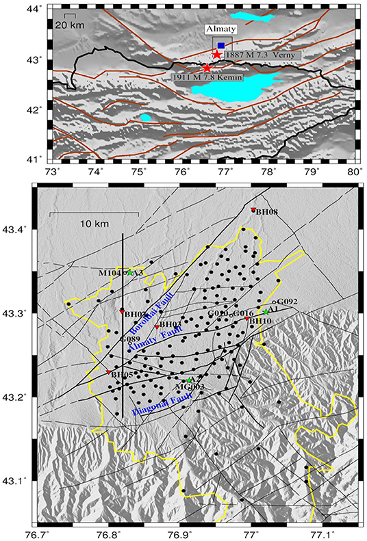
Figure 1. (Top) Main faults (brown lines) in and around the study area (thin black line rectangle). The main historical earthquakes that affected Almaty are indicated. (Bottom) Study area (red stars). Black circles depict the location of the 170 single station noise measurements used in this study. The inverted red triangles indicate the location of the analyzed boreholes. Green stars indicate the location of the seismic noise measurements using small arrays. The vertical thick black line indicates the cross section discussed and shown in Figure 12. Thin black lines show the surface locations of known faults. The urban area is indicated by a yellow line.

The Paleozoic basement is close to the surface in the mountainous sectors located in the south of the area. In the relatively flat northern side of the depression, the basement has a depth of around 2,200 m in the northeastern sector and 1,800 m in the northwestern sector.

Within the city's territory, the basement is divided into separate blocks by NE-SW and NNE-SSW striking faults. The Almaty Fault, which crosses its central part, and the Zailiysky Fault, crossing the southern part, are included in the system of faults separating the Almaty depression from the Zaili Alatau. The northwestern sector of the depression is confined by the Boroldai Fault, whereas the southeastern part is dissected by the NE striking Diagonal fault (Figure 1).

The major faults crossing the city's territory have not been associated with any previous historical event, but might have the potential to generate a large earthquake in the future. In a previous study, Pilz et al. (2015) showed that amplification of ground motion occurs at low frequencies of around 0.1–0.2 Hz due to the strong impedance contrast between the Paleozoic sediments and the seismic bedrock. Such amplification effects at low frequencies are particularly dominant in the central and north-western parts of the city. The lowest fundamental resonance frequencies at around 0.08 Hz are found in the central-eastern parts of the city, where the thickness of the sedimentary cover made up of Paleozoic and more recent deposits reaches up to 3.7 km (Shatsilov, 1989). Here, the soils are characterized by soft clay deposits and sandy loams, giving rise to high amplification values. A further clear peak in the range between 0.5 and 1 Hz, which might be interpreted as being due to a shallower impedance contrast, can be found for all measurement sites. These peaks, both for the frequency range of interest and the results of a visual inspection of the vertical and horizontal components spectra are without any doubt of natural origin. In addition, peaks at frequencies higher than 10 Hz can be identified for all the investigated sites in the central part and the northern districts of the city, where soils with low stiffness (sandy loams and sands of different coarseness) are predominant. Thin layers within the overlying formation (thicknesses from 5 to 20 m) are predominant there. Finally, Pilz et al. (2018) showed the existence of 2D/3D site amplification within the basin, indicating the necessity to complement standard seismic hazard assessments with numerical simulations of ground motion that consider a 3D model of the basin structure. The approach proposed in this paper aims to provide a tool for deriving, in future studies, a 3D model of the basin.

Data

In summer 2014, 15 weak-motion instruments (Guralp CMG-3ESP broadband sensors) were temporarily deployed in the area of Almaty for recording seismic noise and earthquakes (Pilz et al., 2015). Using this equipment and additional short-period (1 Hz) sensors, around 220 measurements of seismic noise were carried out in the urban area, with an average spacing of 1 km (Figure 1). Recordings at each site were carried out during the day time for safety reasons and for a duration of not <60 min. Small arrays were used in three locations within the city to estimate the S-wave velocity profile (Figure 1).

Regarding the single station noise measurements, the recordings were first divided into 3-min length windows, tapered 5% at both ends, then Fourier transformed, smoothed with a Konno and Ohmachi window (b = 40) (Konno and Ohmachi, 1998), after which the H/V was calculated. An average H/V is then calculated considering the results of several 3-min time segments. At some of the stations, where a broadband sensor was installed, single station noise measurements were carried out to compare the compatibility of the results. Note that Strollo et al. (2008) showed the capability of 1 Hz short-period sensors to work reliably down to 0.1 Hz. The window length was chosen to be 180 s in order to obtain reliable results for the low-resonance frequencies expected considering the outcomes of previous studies (Pilz et al., 2015). We observed that the results obtained with the two different sensors were nearly the same (depending on the existing seismic noise level) down to 0.1 Hz. Below 0.1 Hz (i.e., down to 0.07 Hz), the shape was similar (peaks were occurring at the same frequencies), but with different amplitudes (Figure 2). This difference may be due to the different response of the sensors (Strollo et al., 2008). Finally, each H/V curve has been assigned a weighting (w0) ranging from 0 to 1 in steps of 0.25, depending on its quality (standard deviation, reliability of the low-frequency tendency, etc.), based on a visual inspection and expert judgment. This qualitative weight will be used in the procedure of interpolation for deriving the 3D model of the area, as described in the following section.

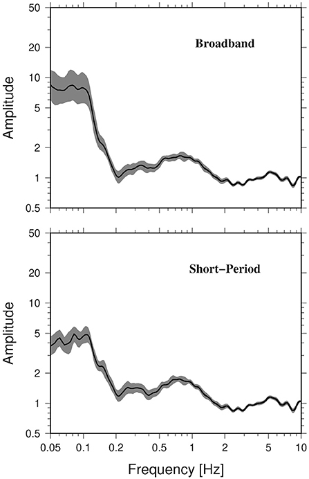
Figure 2. Examples of H/V curves for broadband and short-period sensors at station MG03. The mean value (black line) and the standard deviations (gray area) for each considered frequency are shown.

Array measurements have been carried out in three different locations (Figure 1) within the area of Almaty, where, in light of existing information, different velocity structures would be expected. In particular, lower S-wave velocities were expected in the shallow sedimentary cover situated to the north of the SW-NE trending Almaty fault located close to the sites denoted as G089, G016, and A1.

Array measurements were carried out with 16 seismological stations and for 120 min duration at each site. Seismic noise data were divided into signal windows of 120 s and the Extended Spatial Correlation Analysis ESAC method (Ohori et al., 2002) was applied. The estimated Rayleigh wave dispersion curves were inverted jointly with the H/V curves following the scheme proposed by Parolai et al. (2005). Figure 3 shows the results obtained for the three locations, confirming lower S-wave velocities in the uppermost 150 m (where the models appear to be better constrained) at sites located in the northern part of the city. Note that from a visual inspection, the fit of the theoretical dispersion curves to the observed ones is always excellent, while the fit of the H/V theoretical curves to the empirical one ranges from good (arrays A1 and A3) to fair (A2). To a first-order approximation, the dispersion curve mainly constrains the velocity model down to a depth corresponding to the maximum wavelength divided by two (about 130, 160, and 50 m, for arrays A1, A2, and A3, respectively). As a result of the variability in the estimated velocities over the same depth range, indicated by the inverted models providing a misfit within the 10% of the minimum one, in the following analysis, only the results down to 150 m were considered. The profiles have been resampled, subdividing each layer into 10 thinner segments with the same velocity, in order to carry out the following analysis (Figure 4).

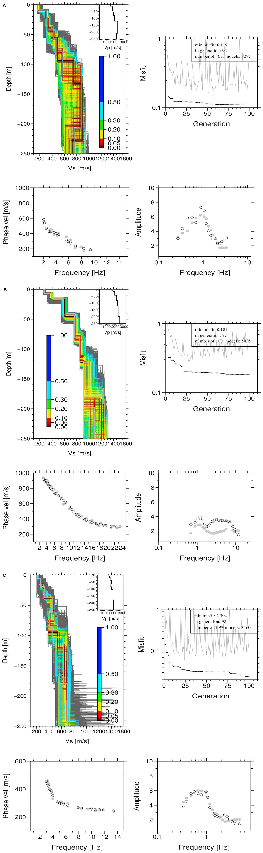
Figure 3. (A) (Top left) Joint inversion for (A1): all tested models (colors indicate models lying within a certain percentage of the minimum misfit), and the minimum misfit model (thick gray). The inset shows the P-wave velocity. (Right top), minimum misfit (black dots), and average misfit (gray line) vs. the number of generations for the seed number leading to the best model. (Right bottom) Observed (gray circles) and calculated (open circles) H/V spectral ratios. (Left bottom) Observed (gray circles) and calculated (open circles) apparent phase velocities. (B) As for (A) but for array (A2). (C) As for (A) but for array (A3).

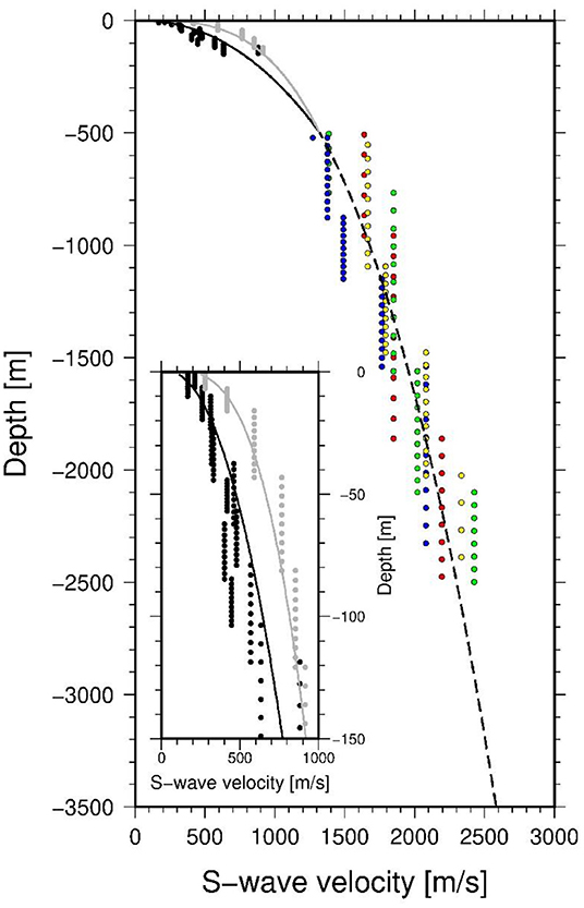
Figure 4. S-wave velocity vs. depth. Black (northern array) and gray (southern array) points show the velocities obtained via seismic noise array measurements. Blue, red, green, and yellow circles show the velocities for depths larger than 500 m obtained by borehole data investigations (BH08, BH01, BH05, and BH10, respectively). The thin gray (southern array) and black (northern array) lines represent the velocity profiles obtained by non-linear fitting for the shallow parts, while the dashed black line shows the velocity vs. depth profile obtained for depths >500 m. The inset shows a zoom of the uppermost 150 m.

Several deep boreholes (crossing the Quaternary and Tertiary sediments and reaching the Paleozoic bedrock down to a depth of more than 3 km) have been drilled in Almaty and the surrounding areas (Silacheva, 2002). Amongst them, in three boreholes lying inside the investigated area, P-wave velocity measurements were also carried out. After a careful re-evaluation of the available data (including an inspection of the available electric logs), it was considered that a reasonable P-wave to S-wave velocity conversion, using a fixed Vp to Vs ratio of √3, was only feasible for depths >500 m. These data have been digitized, and resampled for each layer by dividing them into 10 thinner segments with the same velocity of the whole layer (Figure 4). The resampling was necessary to provide a sufficient number of velocity vs. depth data points to the procedure used to define reference profiles for the area explained in the following chapter.

Deriving 1D Smooth Reference S-wave Velocity Profiles

First, an S-wave velocity profile for depths >500 m (the depth for all boreholes that is below the soft layer material) was derived by fitting the velocity values obtained from borehole measurements over the 500–2,500 m range (Figure 4). The fit was carried out using a non-linear least-squares (NLLS) Marquardt-Levenberg algorithm, considering the function (Ibs-von Seht and Wohlenberg, 1999; Parolai et al., 2002a):

where vs(z) is the calculated S-wave velocity vs. depth z in m, vs0 is the S-wave velocity at the surface, and x defines the gradient for the increasing velocity. Note that the z values are defined as being positive downward.

Following this approach, the best fit for the borehole data was obtained for vs0 (from here on defined as vs02) equal to 155 m/s and x (from here on defined as x2) equal to 0.344 (Figure 4).

Considering that the northern and southern shallow velocity profiles show consistently different velocities, it was decided to derive two reference profiles for the proposed method to highlight the presence of impedance contrasts leaving a fingerprint in the H/V.

In order to obtain the shallow velocity profiles, and to combine them in a harmonized way with the obtained deeper ones, the northern and southern velocity points have been fitted separately by means of a linear inversion using the Singular Value Decomposition (SVD) algorithm (Press et al., 1986).

To do this, Equation (1) is transformed by taking the logarithm of its components

and the inversion is carried out by constraining the value of the S-wave velocity at 500 m to be equal to 1,321 m/s, which is the velocity obtained at that depth by fitting the borehole data (i.e., using the coefficients vs02 and x₂) (e.g., Parolai et al., 2000).

The two obtained smooth reference velocity profiles (Figure 4) show a very good fit to the data. The southern profile (with vs0 = 202 m/s and x = 0.302) clearly reproduces the trend of the higher velocities vs. depth relative to the northern one (vs0 = 81 m/s and x = 0.450).

Method

In this section, the procedure followed to transform the H/V spectral ratio from the frequency to the spatial domain using the references profiles will be illustrated. The procedure is valid when the velocity structure can be represented in one or two depth intervals by the Equation (1) model. Furthermore, a description about how to extract the major impedance contrast fingerprints from the H/V vs. depth curves will be provided. Finally, the procedure followed to derive a 3D model of the impedance contrast related fingerprints will be described.

H/V Migration

In this study, we proposed a means of migrating the H/V spectral ratio to depth. A sketch of this procedure is presented in Figure 5. To do this, we describe the velocity variations with depth via Equation (1). If the depth z is less than the depth H (0 < z < H) where a change in the equation that models the velocity profile is expected (for the case at hand 500 m) the travel time t(z) of the S-wave through the velocity profile can be calculated as:

where vs0₁ is the velocity at the surface and x has the same value as in Equation (1).

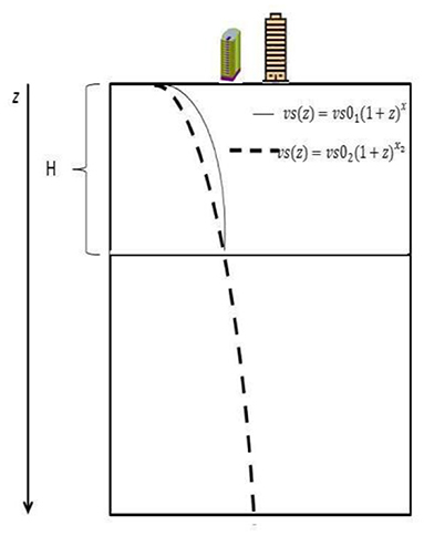
Figure 5. Sketch showing the basics of the procedure proposed. H is the thickness of the shallow structure that can be represented by the first gradient model.

It follows that:

and, after a further step:

In the case where z = H, then,

Under the first-order approximation that any peak in the H/V might indicate a resonance frequency f_r determined by an interface at a certain depth, the frequency can be related to the depth through the travel times as (e.g., Joyner et al., 1981):

Combining Equations (5) and (7), for $f_r\ge \frac{1}{4t(H)}$, we obtain:

For depths greater than the thickness H (z > H), the travel time over the interval z-H must be estimated. First, considering that if the second depth-interval parameters are used (vs0₂ and x₂), the total travel time t₂(z) between the surface and z is expressed by:

Solving for the integral one obtains:

and for the depth H:

Second, the travel time Δt between H and z can be calculated as:

Finally, the total travel time t(z) is estimated by combining Equations (6) and (12)

Considering the relationship between the resonance frequency and depth (Equation 7), one can write:

and therefore obtain:

It then follows that:

and

Finally, the depth (z) at which each amplitude in the H/V spectra ratio can be assigned, dependent upon the frequency and the estimated velocity profile, is given by:

Fingerprint Identification

In order to highlight the peaks in the H/V that are expected to indicate the presence of impedance contrasts at depth, we propose a procedure similar to that introduced by Wüster (1993) and applied by Parolai et al. (2002b) for identifying particular features in sonograms. A similar approach was also used by Yoon et al. (2015) for earthquake detection.

In the proposed approach, the visibility of local peaks in the H/V is improved by smoothing the spectral ordinated using a Konno and Ohmachi (1998) window with two different values of the parameter b, which defines the degree of smoothing. After trial and error tests, we set the parameter b for the low level of smoothing to 30, and for the high level of smoothing to 5.

The difference between the logarithms of the low- and highly-smoothed estimates at each frequency in the average H/V ratios is calculated and then considered as an indication of a local peak (if positive). Each difference estimate is normalized with respect to the maximum one obtained at each station and stored. This is different from Wüster (1993) who simply stored them by assigning a value of 1 if the value is positive and 0 to all the others.

This procedure allows the peaks which might have different amplitudes in the original H/V ratio, to be better highlighted relative to the impedance contrasts. At the same time, it permits the improvement of the spatial coherency of the peaks occurring at the same frequency, but with different absolute amplitudes in the original H/V at different stations. Figure 6 shows some examples of the H/Vs, the results of the low and high smoothing procedure, and the highlighted spectral peaks. Note how the proposed procedure is able to highlight even relatively small features in the H/V curve, independent of its local amplitude. For the sake of completeness, the weights (w0) assigned to the H/V curves shown are 0.5, 1, 0.75, 1, 0.5, and 1, for the stations M104, G089, MG003, G010, G016, G092, respectively.

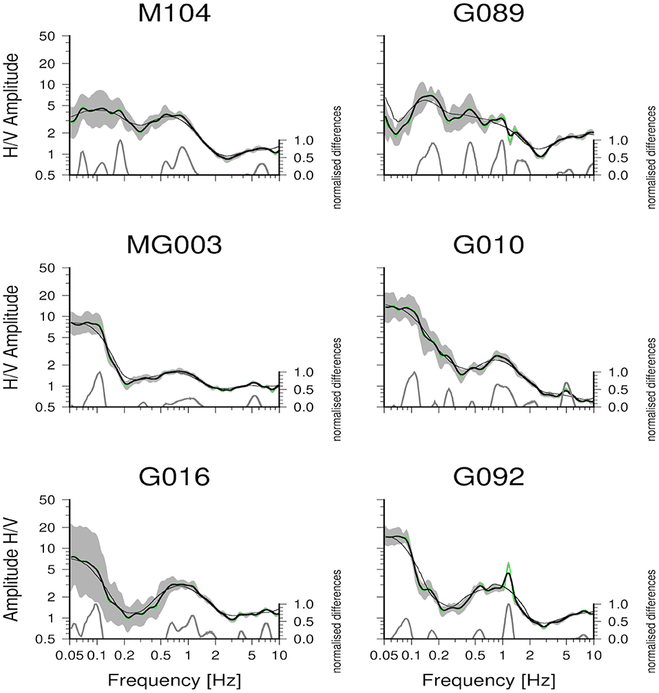
Figure 6. Examples of the H/V spectral ratios (green line—mean value, gray area—the standard deviation), high and low levels of smoothing of the H/V spectral ratios (thin and thick black lines, respectively), and extracted fingerprints (gray lines).

The capability of the procedure to retrieve the main impedance contrasts at depth was tested by using numerical simulations. Here the results obtained by computing the H/V spectral ratios for a model with two layers (Vs = 600 and 1,200 m/s, H = 250 and 1,250 m) and a half space (Vs = 2,000 m/s) (Figure 7) are reported. A reference profile was computed considering Equation (1), the H/V ratio was migrated and the fingerprints extracted, following exactly the same procedure used for the real data (note that in this case only one reference profile was used). Figure 7 shows that the proposed approach is able to identify clearly the two impedance contrasts existing in the considered model, while their depths are overestimated by nearly 30 and 20% for the shallowest and deepest contrasts, respectively. The total uncertainty is the result of a combination of the lack of accuracy (closeness of the estimate to the real depth of the impedance contrast) and precision (indicated by the sharpness of the fingerprint feature). The lower accuracy for the shallower impedance contrast is due to the fact that Equation (1) describes a model that poorly represents a layer with a constant velocity. The accuracy increases with depth because Equation (1) better represents the trend of the velocity vs. depth over the larger (0–1,500 m) depth interval. However, the broadening of the fingerprint features with depth, indicating diminishing precision, is related to the equispaced sampling in the frequency domain of the spectrum. In fact, due to the non-linear relationship between frequency and depth [Equations (8) and (18)], the same step in frequency can generate very different steps in depth, when the low- or high-frequency range is considered. Since in real cases the velocity is expected to increase with depth due to the overburden pressure effect, a 20% error in the impedance contrast position might represent an upper boundary of the uncertainty. This value, as also observable in Figure 7, is certainly acceptable when mapping basins for seismic hazard analysis, in particular when considering that it allows one to obtain information at a lower cost and over large urban areas.

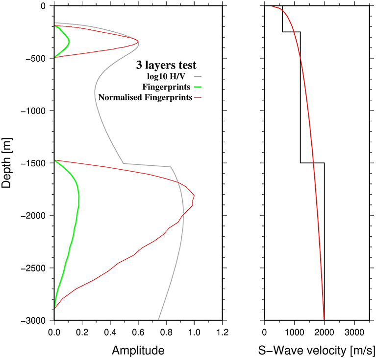
Figure 7. (Left) Initial synthetic H/V spectral ratios (gray thin line), extracted fingerprints (green line), and normalized fingerprints (red line). (Right) Vs model (black) for the calculation of the synthetic H/V spectral ratios and gradient velocity model (red) used to approximate it. For further explanation, please refer to the main text.

Deriving the 3D Subsurface Model

Using Equations (8) and (18), the H/V spectral ratio, modified after the fingerprint identification procedure, were transformed from the frequency to the depth domain. An example is shown in Figure 8 for depths until 2,000 m. Note that the proposed procedure clearly highlights the features existing in the spectral ratio and that the normalization (while keeping the relative importance of the peaks) will allow a more efficient spatial correlation of the identified features.

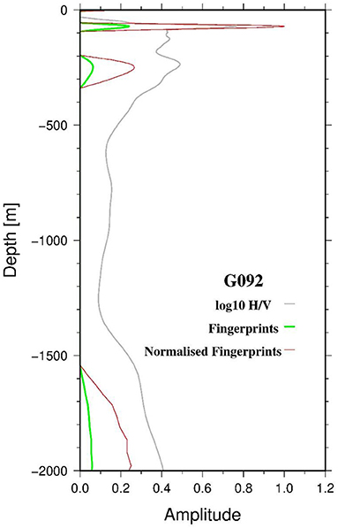
Figure 8. Example of the initial H/V spectral ratio (gray thin line), extracted fingerprints (green line), and normalized fingerprints (red line) for the G092 site. For further explanation, please refer to the main text.

Note also the widening of the peaks with depth due to the equally spaced frequency samples in the Fourier transform combined with the non-linear relationship between frequency and depth. Applying the proposed procedure, for each individual noise measurement site, a profile showing impedance contrasts vs. depth was obtained. In order to derive a 3D model for the area that accounts for the irregular spatial sampling of the measurements, the calculated profiles have been interpolated onto a 3D regular grid (Figure 9).

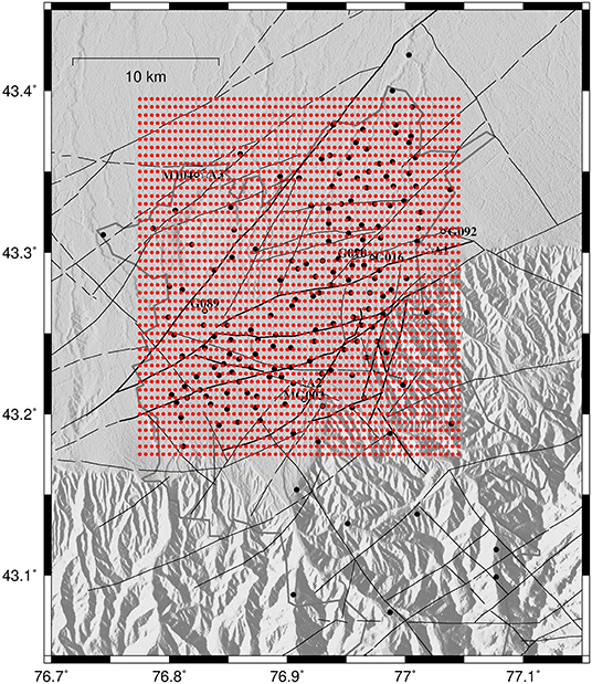
Figure 9. Study area. Black circles depict the position of the single station noise measurements. Thin black lines show the surface position of known faults (see also Figure 1). Red circles indicate the grid points along the surface used for the interpolation.

The grid points are spaced regularly every 0.005° in both latitude and longitude in the horizontal plane, and by 10 m in the vertical direction. In order to account for the larger sparsity of information on the horizontal plane (due to the distance between the individual noise measurement sites) with respect to the vertical direction (due to the resolution of the vertical profiles), the following strategy for resampling was proposed.

The value assigned to each grid point is calculated as a weighted average of the measurement points by:

where v_est(x,y,z) is the value estimated for a grid point, v(x_i,y_i,z_i) is the value of the normalized fingerprint at each measurement site at a certain depth, N is the total number of values considered (i.e., number of measurement sites multiplied by the number of considered depths in each profile), w0_i is a weighting factor that depends on the quality of the H/V (and therefore is the same for each site, independent of depth), and w1_i is a distance weighting factor calculated by:

where dh_i is the horizontal distance of the considered v(x_i,y_i,z_i), and d_ref is a reference distance beyond which w1_i is set equal to 0. The value of the exponent was set to 6 after trial and error tests.

W2_i is a depth weighting factor calculated by:

where a is:

and a_ref is a reference value, beyond which w2_i is set equal to 0, z_i is the depth of the considered value at the measurement site i and z is the depth of the considered grid point. In this study, d_ref and a_ref have been set, after trial and error tests, to 3 km and 0.2, respectively. These values allow a good compromise between the requirement of sufficient spatial interpolation and retaining information on the local input normalized fingerprint values. Of course, the results in areas at the edge of the model, or with a low density of measurement-points will be strongly extrapolated, leading to horizontal stretching of the nearby features. The interpretation of the results must therefore take this issue into account.

Results

The derived 3D subsurface model is shown in Figure 10, after having corrected it for elevation, provided by the SRTM topography model (Becker et al., 2009). The resulting subsurface model shows several possible interfaces occurring at different depths and with quite marked lateral discontinuities.

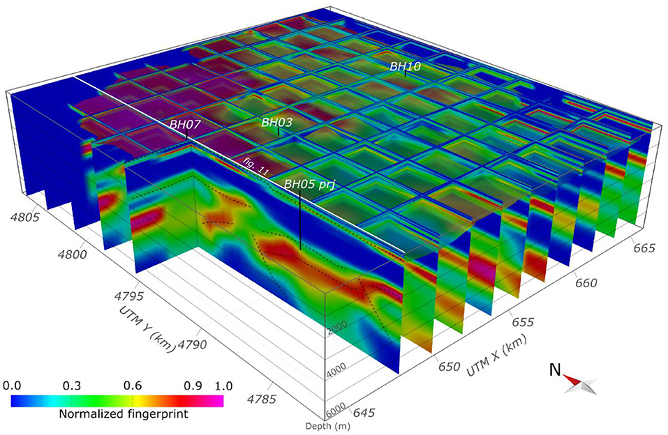
Figure 10. Fence diagram derived from the 3D model with 2 km spaced sections. Solid back lines indicate the boreholes' positions. Note that borehole BH08 is located outside the area covered by the model. Thin dashed lines are an example of the interpretation of horizons and faults (see Figure 11 for more details).

In order to interpret the identified features, a calibration of the depth migrated H/V ratios was carried out using the available data from four deep boreholes (maximum depths of nearly 3,000 m) in the area (Silacheva, 2002). Within each borehole, five geological markers delimiting the major stratigraphic units (Figure 11) were observed:

(1) Top PL is the boundary between the Pleistocene sequence on the top (with Vp velocities estimated by the borehole investigation ranging between 2,200 and 2,300 m/s) and the upper Pliocene sequence (Vp~2,800–2,900 m/s). This feature has been identified in all boreholes.

(2) Top ZAN separates the upper Pliocene sequence from the late Miocene—lower Pliocene sequence (Vp~3,400–3,600 m/s). This marker was identified in all boreholes. In BH07, it reaches a shallower depth, with its base located just below the top ZAN marker.

(3) Three boreholes (BH10, BH05, and BH03) show the presence of a marker within the Miocene (intra MIO) (deepest part with Vp ranging between 3,600 and 4,018 m/s) with an uncertain age attribution.

(4) The same boreholes also showed a marker at the top of the Paleocene-Oligocene succession (top OL) (Vp measurements showed a large variability with values ranging between 3,000 and 4,200 m/s).

(5) Finally, the basement marker (top BAS) is intercepted only by boreholes BH03 and BH05. The basement P-wave velocity was estimated to be ~5,800 m/s.

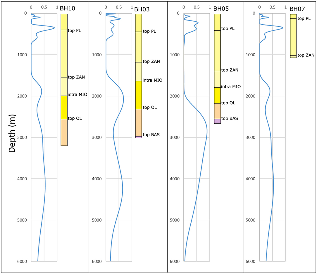
Figure 11. Correlation between borehole stratigraphy (Silacheva, 2002) and normalized fingerprints' values.

The comparison of the depth-migrated H/V features with the available borehole stratigraphy highlighted that the position of the top PL was very well-identified in boreholes BH10 and BH05. The Pleistocene succession above the top PL marker is characterized by some features (small amplitude peaks), probably indicating the existence of vertical impedance contrasts. Note that in BH03, the extracted features seem to indicate smaller impedance contrasts, due to their smaller amplitude, with respect to the other boreholes.

The BH07 stratigraphy is characterized by a reduction in the thickness of the Pleistocene succession. The highest amplitude of the depth-migrated H/V fingerprints is located within the upper Pliocene succession and does not correspond to the top PL marker. This might be due to either lateral changes in the velocity that may lead to errors in the vertical positioning of the features, or to the approximation in the interpolations carried out to derive the 3D model. However, we cannot exclude the contribution of the uncertainties associated with the age attribution of the stratigraphy of the boreholes.

The correspondence between the borehole stratigraphy and the extracted features becomes less obvious with depth, both because the depth-migrated H/V fingerprints are broadening with depth as a result of the frequency-velocity relationships, and also because of possible lateral variations in the lithology, which might affect the quality of the reconstruction with depth. It is, however, remarkable that in all boreholes, the top ZAN horizon does not lead to any significant feature that can be extracted by the H/V, probably indicating a lack of significant impedance contrast between this and the PL layer.

Boreholes BH10 and BH03 show a broad feature between the top OL and the intra MIO horizons. This feature is not clearly present in borehole BH05, where instead a clear feature (a peak) is located close to the bottom of the borehole near the top BAS horizon.

The top BAS horizon is also reached by the BH03 borehole. It is questionable, however, whether the shallower feature indicated above could indicate this horizon, therefore highlighting the uncertainties in the migration of the H/V, or if the BAS horizon was really reached during drilling. In this case, the deeper feature, although with the uncertainty growing with increasing depth implicit in the equation used for migration, could represent the deeper top BAS interface.

Having this in mind, in order to map the possible lateral continuities/discontinuities of the identified interfaces, and to provide the first interpretation of the results, different sections with N-S and W-E orientation and 2 km spacing were extracted from the interpolated 3D model (Figure 10). Next, the spacing of the section was decreased, in particular in the vicinity of the boreholes. First, the top PL was mapped as the lowermost (and highest amplitude) feature in the shallower part of the sections, except for the sections intersecting BH07, where the high amplitude shallow feature is considered to be representative of an impedance contrast within the upper Pliocene sequence. The top OL and top BAS horizons cannot be mapped with the same precision as the top PL because they are represented by a wider and smoothed signal with an approximate correlation with the boreholes. In that case, we limited our interpretation to the mapping of a positive amplitude signal near the top of the basement (near top BAS) across the model. The lack of lateral continuity of the derived feature was tentatively interpreted to be due to fault displacement.

Figure 12 shows, as an example, the interpretation of a cross section. A detailed interpretation of the basin structure is beyond the scope of this paper, which is mainly focusing on describing the proposed innovative approach and its feasibility in reconstructing, at a low cost, but with sufficient detail, a basin's structure. Figure 12 shows that it is possible to identify folding in the high amplitude feature at around 2,000 m depth in the southern termination of the profile. Considering the known tectonics of the area, this folding has been related to a south-dipping reverse fault. The sharp discontinuity in the central part of the section has been interpreted as a high angle fault that is steeply dipping to the North.

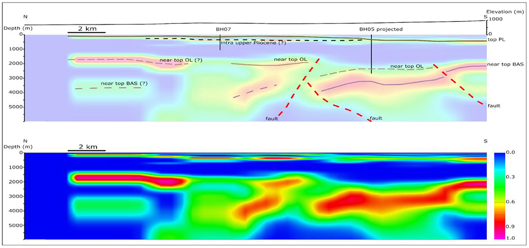
Figure 12. Example of interpreted (Top) and uninterpreted (Bottom) cross section in the 3D model. The color scale represents the normalized fingerprint values.

Furthermore, Figure 12 suggests that the top PL horizon is deeper, corresponding to borehole BH05, and is much shallower in borehole BH07, in agreement with the borehole stratigraphy. The high amplitude feature (marked by the intra upper-Pliocene layer in the section) between BH07 and BH05, already discussed above during the calibration procedure, can be followed with good continuity to both the north and south where it connects with the top PL horizon. This geometry suggests the possible presence of a Pliocene depocenter with a lithological contrast in the deep part of the northern half of the section.

As an example of the spatial reconstruction of the geological horizons, Figure 13 shows the top PL horizon and the “near top BAS” horizon extending across the area, both with respect to the datum [Datum = 0 elevation a.s.l. (m) of each point at the surface of the model] (Figure 13A) and after the topographic correction. The map of the top PL (Figure 13B) highlights the presence of a relative structural high in the NW sector. Even if it is less clear, the same relative high is also present in the “near top BAS” map (Figures 13C,D) and is limited by a NE-SW trending lineament corresponding to the Borolai Fault already mapped in the area (Kurskeyev et al., 1993). Considering the section depicted in Figure 12, this fault seems to be a high angle reverse northward-dipping fault that possibly inverted an upper Pliocene basin located at the front of the northerly-verging thrust and that activated during the Pleistocene.

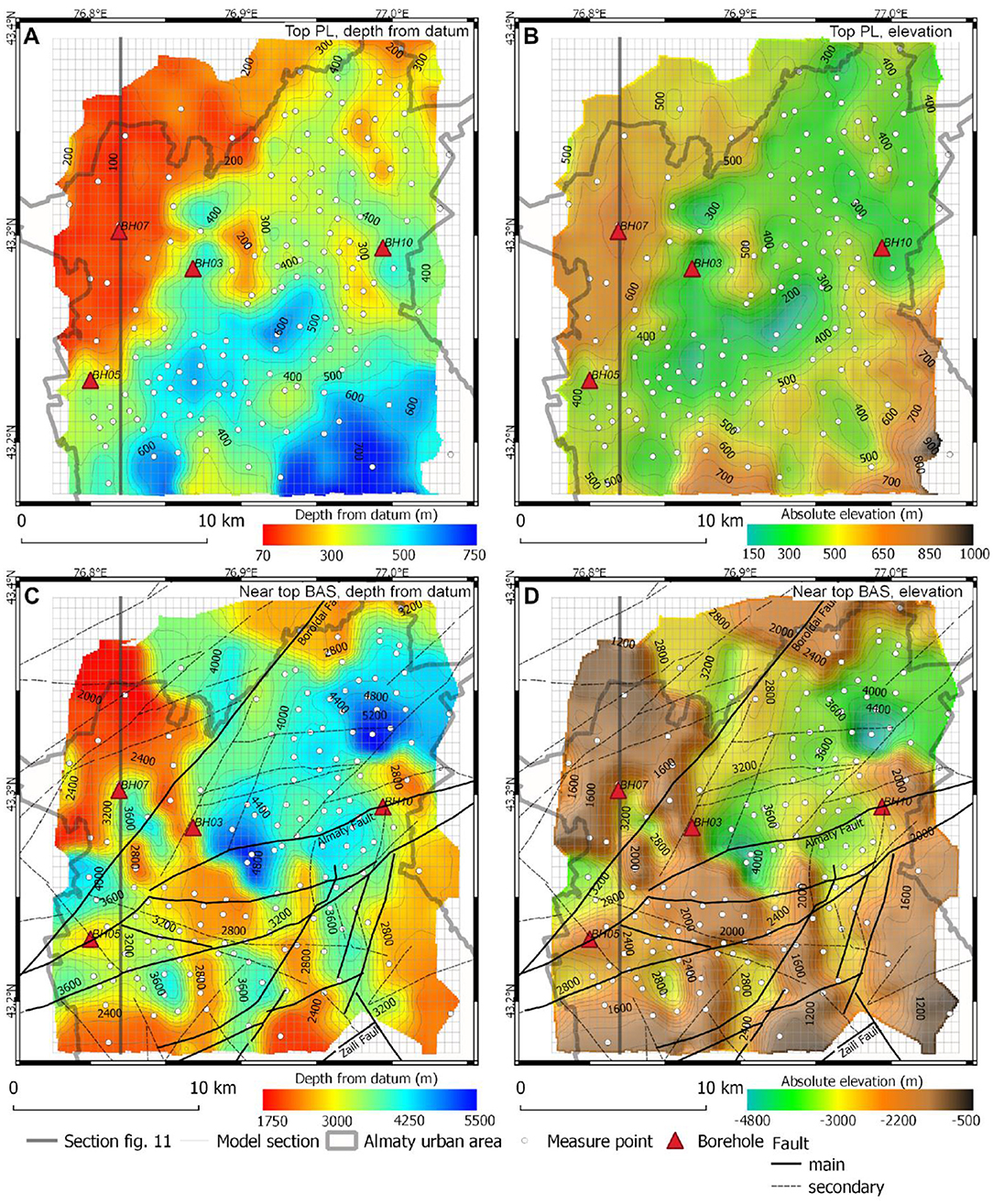
Figure 13. (A) Map of the top PL horizon relative to the model datum [Datum = 0 elevation a.s.l. (m) of each point at the surface of the model] and (B) after being corrected for the absolute elevation (SRTM, Becker et al., 2009). (C) Map of the near-top BAS horizon relative to the model datum [Datum = 0 elevation a.s.l. (m) of each point at the surface of the model] and (D) after being corrected for the absolute elevation. The faults traces in (C,D) are with respect to the basement and are the same as reported in Figure 1.

Similarly, the southeastern part of the model is characterized by a structural high bounded by faults pertaining to the Diagonal Fault system, whereas the role of the Almaty Fault, located in the central part of the basin, in shaping the top PL and near-top BAS horizons is less clear.

Figure 13B shows the top of the PL horizon position after correcting for topography. Since the elevated topography is located along the southern and southeastern margins of the study area (Figures 1, 9), this correction mainly affects this area. Please note that the relative low shown in Figure 13A becomes a relative high in Figure 13B after the correction for topography. The morphology of the horizon in the central part of the area is not affected by the correction since it is an almost flat zone. The central part of the study area has a syncline morphology located between the relative highs in the southern sector and the high in the northwestern sector already visible in Figure 13A.

Conclusions

In this study a new approach for extracting features related to depth-dependent impedance contrasts from the H/V spectral ratio of seismic noise was proposed. The approach relies on migrating the H/V spectral ratio from the frequency domain to the depth domain once an S-wave velocity with depth profile is available. The main features, representing possible impedance contrasts at depth, are then extracted using a fingerprint identification procedure.

The proposed approach has been applied, exemplarily, using the H/V spectral ratio derived by seismic noise measurements in the urban area of Almaty. In this area, S-wave velocity profiles are available from array measurements and borehole log data. Using inversions and regression of the available data, initial S-wave velocity profiles have been derived and used for migrating the H/V spectral ratio with depth. The features extracted by the procedure are then interpolated to obtain a 3D model of the impedance contrasts existing in the subsoil.

After a comparison with available borehole log data, it was found that the proposed procedure is able to identify the main lithological variations with depth. Higher resolution and lower uncertainties are observed for the shallower impedance contrast by comparing the results with borehole data. This evidence seems to contrast with the results of the synthetic tests, where the uncertainty at shallow depths, due to a lack of accuracy, appears to overstep that related to the precision. We think that this is due to the fact that the synthetic model used in the test (having thick constant velocity layers close to the surface) only roughly approximates reality and, as discussed above, the Equation 1 model fails to represent this shallow synthetic velocity structure. It is therefore reasonable that in real cases, where the velocity is expected to increase generally with depth, the error in the position estimation of the impedance contrasts might be dominated by the precision that, as explained above, is determined by the equispaced sampling in the frequency domain of the Fourier transform and the non-linear relationship between frequency and depth. Further testing with additional numerical simulations should be carried out especially for areas with more complex geological settings.

The limits in the vertical resolution (20% at greater depths) are considered acceptable if one takes into consideration the reduced required efforts and cases where highly resolved results (meters scale) are not necessary. Furthermore, when applied to the Almaty area, the method was able to reproduce the morphology of the main geological horizons and, after comparisons with available data, to identify the main faults in the area. Although a comprehensive reconstruction of the basin is well-beyond the scope of this paper, we think that the results of the proposed procedure, after a due comparison with all available geological and geophysical data, will allow a detailed reconstruction of the 3D geometry of the main geological horizons. Furthermore, they will permit the better resolution the depth (and lateral continuity) of the faults in the area. Such a model will provide an important contribution for improving seismic hazard and risk assessment in Almaty, allowing the use of 3D numerical simulations of ground motion. Future work in different test sites is therefore necessary to further validate the proposed procedure for different tectonic and geological settings.

Data Availability Statement

The raw data supporting the conclusions of this article will be made available by the authors, without undue reservation, to any qualified researcher.

Author Contributions

SP developed the proposed approach, carried out most of the calculations, and wrote the manuscript. FM and RB interpreted the results and contributed to the manuscript writing. NS support the results interpretation and contributed to the manuscript writing. MP and TB acquired the field data. MP participated to the writing. TB carried out some analysis on the acquired array data.

Conflict of Interest

The authors declare that the research was conducted in the absence of any commercial or financial relationships that could be construed as a potential conflict of interest.

Acknowledgments

We thank D. Bindi for support in the field activities and stimulating discussions. We thank the two reviewers for their comments and suggestions that improved the manuscript. K. Fleming kindly improved our English. Instruments were provided by the Geophysical Instrumental Pool Potsdam (GIPP) and by the Central Asian Institute for Applied Geosciences (CAIAG). This research has been supported by the Global Change Observatory Central Asia of the GFZ, the Earthquake Model Central Asia (EMCA). Some figures were made using the Generic Mapping Tools version 5.4.5 (www.soest.hawaii.edu/gmt; Wessel and Smith (1998), last accessed December 2019).

References

Bard, P. Y. (1999). “Microtremor measurements: a tool for site effect estimation,” in The Effects of Surface Geology on Seismic Motion, Vol. 3, eds K. Irikura, K. Kudo, H. Okada, and T. Sasatani (Rotterdam: Balkema), 1251–1279.
Becker, J. J., Sandwell, D. T., Smith, W. H. F., Braud, J., Binder, B., Depner, J., et al. (2009). Global bathymetry and elevation data at 30 arc seconds resolution: SRTM30_PLUS. Mar. Geod. 32, 355–371. doi: 10.1080/01490410903297766
Bogdanovich, K. I. (1911). “An earthquake of December 22, 1910 (January 4, 1911) in northern chains of the Tien Shan between Verny and Issyk-Kul,” in Proceedings of Geological Committee (Moscow), 329–419.
Bogdanovich, M. M. C., Kark, J., Korolkov, B., and Muchketov, D. (1914). Earthquake of the 4th January 1911 in the northern districts of the Tien Shan. Tr. Geol. Com. Ser. 89:270.
Castellaro, S., and Mulargia, F. (2014). Simplified seismic soil classification: the Vfz matrix. Bull. Earthq. Eng. 12, 735–754. doi: 10.1007/s10518-013-9543-3
Field, E., and Jacob, K. (1993). The theoretical response of sedimentary layers to ambient seismic noise. Geophys. Res. Lett. 20, 2925–2928. doi: 10.1029/93GL03054
Ibs-von Seht, M., and Wohlenberg, J. (1999). Microtremor measurements used to map thickness of soft sediments. Bull. Seismol. Soc. Am. 89, 250–259.
Joyner, W. B., Warrick, R. E, and Fumal, T. E. (1981). The effect of Quaternary alluvium on strong ground motion in the Coyote Lake, California, earthquake of 1979. Bull. Seismol. Soc. Am. 71, 1333–1349. doi: 10.3133/ofr81353
Kanai, K. (1957). Semi-empirical formula for the seismic characteristics of the ground. Bull. Earthq. Res. Inst. 35, 309–325.
Konno, K., and Ohmachi, T. (1998). Ground-motion characteristics estimated from spectral ratio between horizontal and vertical components of microtremor. Bull. Seismol. Soc. Am. 88, 228–241.
Kurskeyev, A., Nurmagambetov, A., Sydykov, A., Mikhailova, N., and Shatsilov, V. I. (1993). Detailed Seismic Zoning of Almaty Industrial Area. Almaty: Novosti Nauki Kazakhstana 1, 21–24.
Mucciarelli, M., and Gallipoli, M. R. (2001). A critical review of 10 years of microtremor HVSR technique. Boll. Geof. Teor. Appl. 42, 255–266.
Mushketov, I. V. (1888). The earthquake of 28 May 1887 in the city Verny. Izv. Imp. Russ. Geogr. Surv. 14:65.
Nakamura, Y. (1989). A Method for Dynamic Characteristics Estimation of Subsurface Using Microtremor on the Ground Surface. Vol 30. Quarterly Reports, Railway Technical Research Institute, 8–12.
Ohori, M., Nobata, A., and Wakamatsu, K. (2002). A comparison of ESAC and FK methods of estimating phase velocity using arbitrarily shaped microtremor arrays. Bull. Seismol. Soc. Am. 92, 2323–2332. doi: 10.1785/0119980109
Parolai, S., Bindi, D., and Augliera, P. (2000). Application of the generalized inversion technique (GIT) to a microzonation study: numerical simulations and comparison with different site-estimation techniques. Bull. Seismol. Soc. Am. 90, 286–297. doi: 10.1785/0119990041
Parolai, S., Bormann, P., and Milkereit, C. (2002a). New relationships between Vs, thickness of sediments, and resonance frequency calculated by the H/V ratio of seismic noise for the Cologne area (Germany). Bull. Seismol. Soc. Am. 92, 2521–2527. doi: 10.1785/0120010248
Parolai, S., Picozzi, M., Richwalski, S. M., and Milkereit, C. (2005). Joint inversion of phase velocity dispersion and H/V ratio curves from seismic noise recordings using a genetic algorithm, considering higher modes. Geophys. Res. Lett. 32:L01303. doi: 10.1029/2004GL021115
Parolai, S., Trojani, M., Monachesi, G., and Frapiccini, M. (2002b). Seismic source classification by means of a sonogram correlation approach: application to data of the RSM seismic network (Central Italy). Pure Appl. Geophys. 159, 2763–2788. doi: 10.1007/s00024-002-8758-z
Pilz, M., Abakanov, T., Abdrakhmatov, K., Bindi, D., Boxberger, T., Moldobekov, B., et al. (2015). An overview on the seismic microzonation and site effect studies in central Asia. Ann. Geophys. 58:S0104. doi: 10.4401/ag-6662
Pilz, M., Parolai, S., Petrovic, B., Silacheva, N., Abakanov, T., Orunbaev, S., et al. (2018). Basin-edge generated Rayleigh waves in the Almaty basin and corresponding consequences for ground motion amplification. Geophys. J. Int. 213, 301–316. doi: 10.1093/gji/ggx555
Press, W. H., Teulkolsky, S. A., Vetterling, W. T., and Flannery, B. P. (1986). Numerical Recipes in Fortran 77: The Art of Scientific Computing. Cambridge: Cambridge University Press.
Shatsilov, V. I. (1989). Methodology for Seismic Hazard Assessment of Territories, Nauka. Almaty: Kazakh SSR, 208.
Silacheva, N. V. (2002). Impact of Geological Conditions in Almaty on the Parameters of Records of Strong Earthquakes. Reports of the National Academy of Sciences of Kazakhstan, Almaty, 71–80.
Strollo, A., Parolai, S., Jäckel, K. H., Marzorati, S., and Bindi, D. (2008). Suitability of short-period sensors for retrieving reliable H/V peaks for frequencies less than 1 Hz. Bull. Seismol. Soc. Am. 98, 671–681. doi: 10.1785/0120070055
Veletzky, S. N. (1911). “An earthquake in Verny town and Semirechie Oblast (Region) of December 22, 1910 and January 4, 1911,” in Proceedings of Emperor Russian Geographical Society, I/IV (St. Petersburg), 113–163.
Vershinin, P. (1889). An Earthquake in Verny Town of Semirechie Oblast (Region). Notes of Western Siberian Division of Emperor Russian Geographical Society, 10, St. Petersburg, 1–23.
Wessel P Smith W. H. F. (1998). New, improved version of the Generic Mapping Tools released. EOS Trans. AGU 79, 579.
Wüster, J. (1993). Discrimination of chemical explosions and earthquakes in central Europe—a case study. Bull. Seismol. Soc. Am. 83, 1184–1212.
Keywords: H/V seismic noise, Almaty basin, site response, impedance contrast, seismic hazard
Citation: Parolai S, Maesano FE, Basili R, Silacheva N, Boxberger T and Pilz M (2019) Fingerprint Identification Using Noise in the Horizontal-to-Vertical Spectral Ratio: Retrieving the Impedance Contrast Structure for the Almaty Basin (Kazakhstan). Front. Earth Sci. 7:336. doi: 10.3389/feart.2019.00336
Received: 08 September 2019; Accepted: 02 December 2019;
Published: 20 December 2019.
Edited by:
Carmine Galasso, University College London, United KingdomReviewed by:
Hadi Ghofrani, University of Western Ontario, CanadaKiran Kumar Singh Thingbaijam, Institute of Seismological Research, India
Copyright © 2019 Parolai, Maesano, Basili, Silacheva, Boxberger and Pilz. This is an open-access article distributed under the terms of the Creative Commons Attribution License (CC BY). The use, distribution or reproduction in other forums is permitted, provided the original author(s) and the copyright owner(s) are credited and that the original publication in this journal is cited, in accordance with accepted academic practice. No use, distribution or reproduction is permitted which does not comply with these terms.
*Correspondence: Stefano Parolai, sparolai@inogs.it