A Multiscale Productivity Assessment of High Andean Peatlands across the Chilean Altiplano Using 31 Years of Landsat Imagery


Abstract
:
1. Introduction
2. Materials and Methods
2.1. Satellite Data
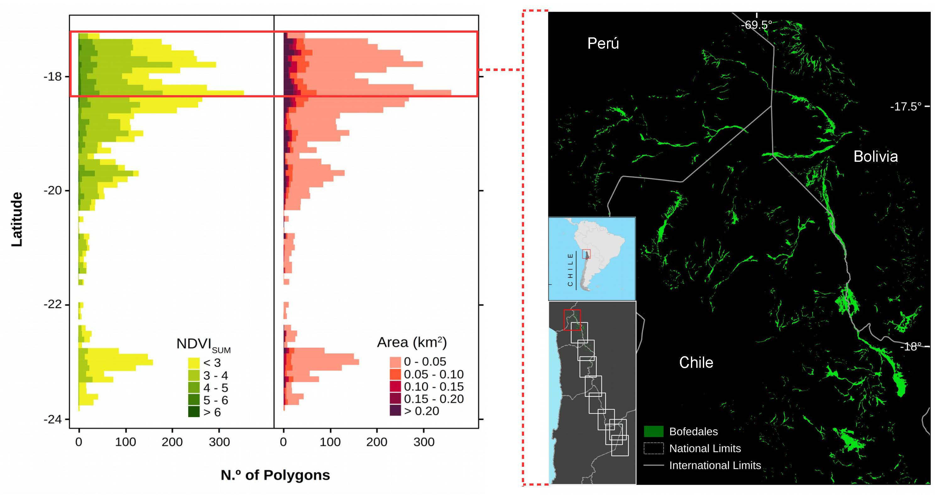
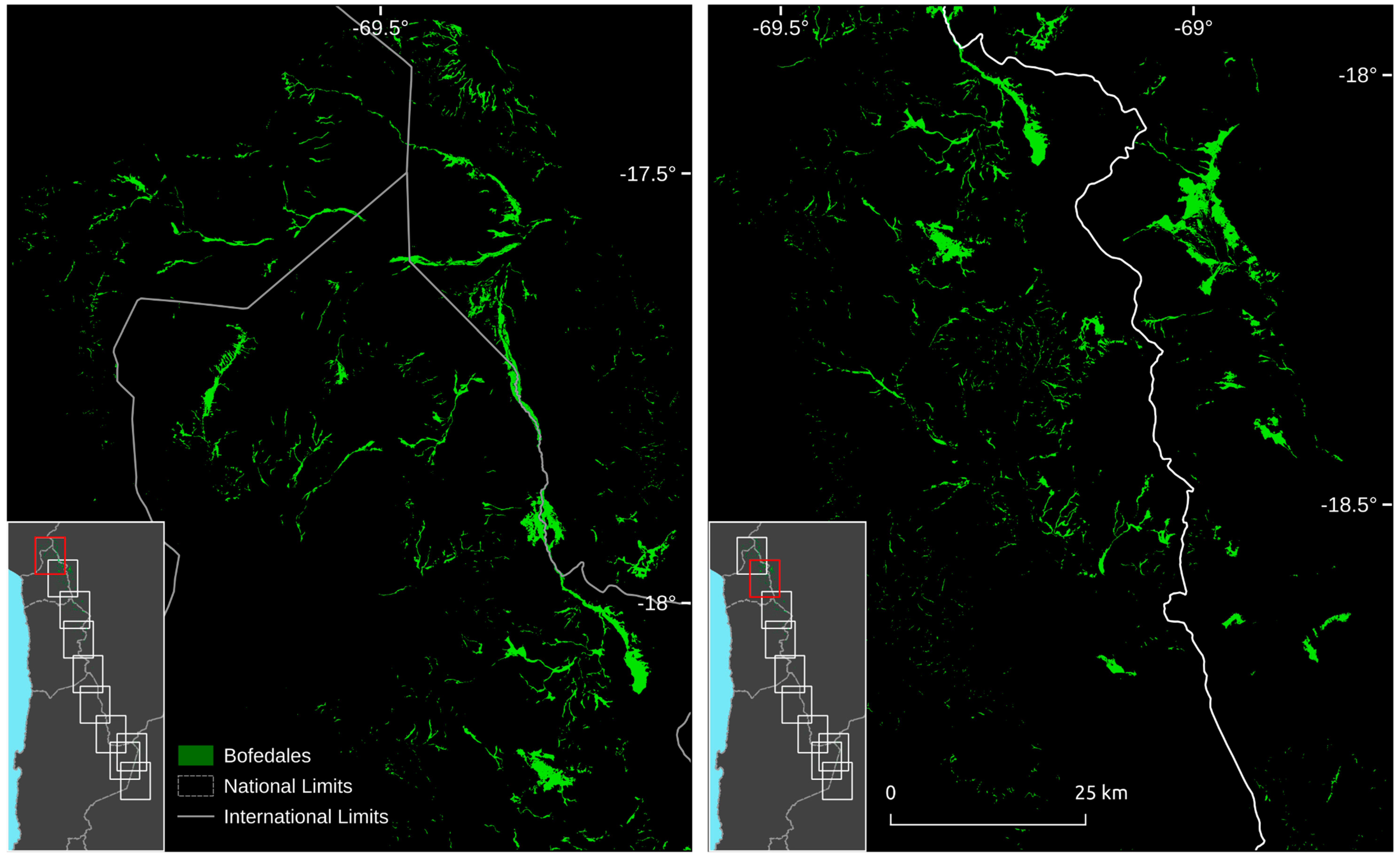
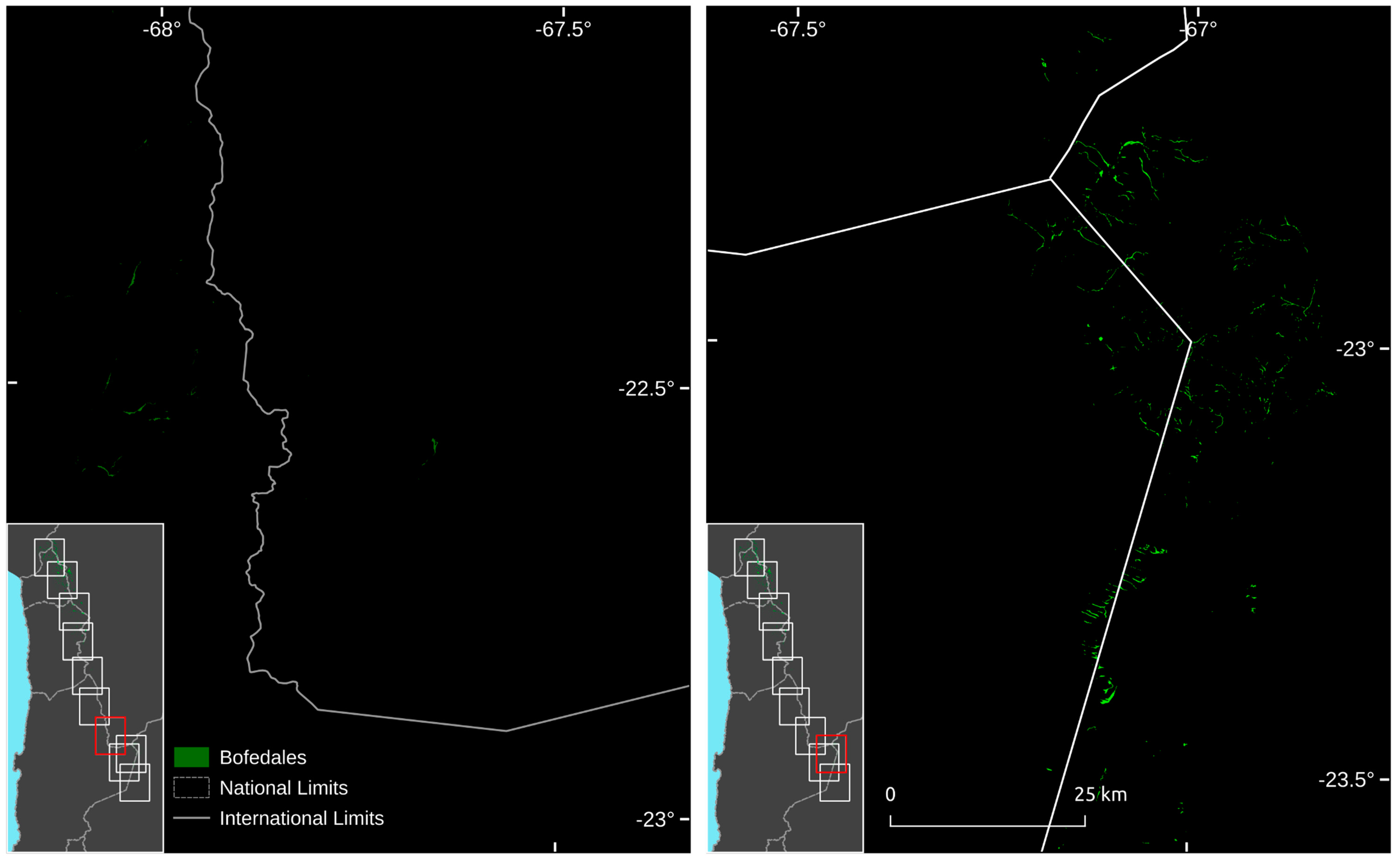
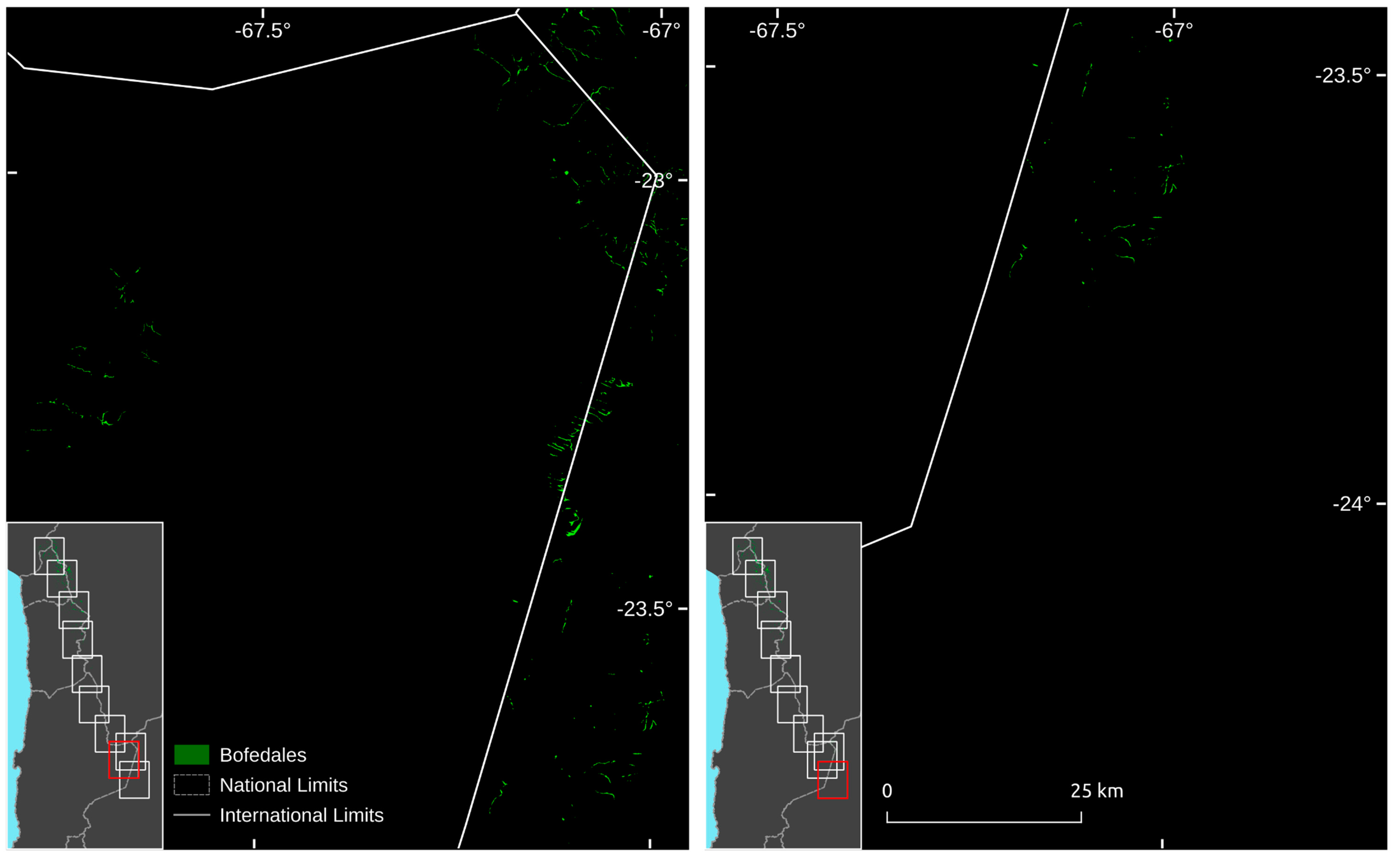
2.2. Study Region
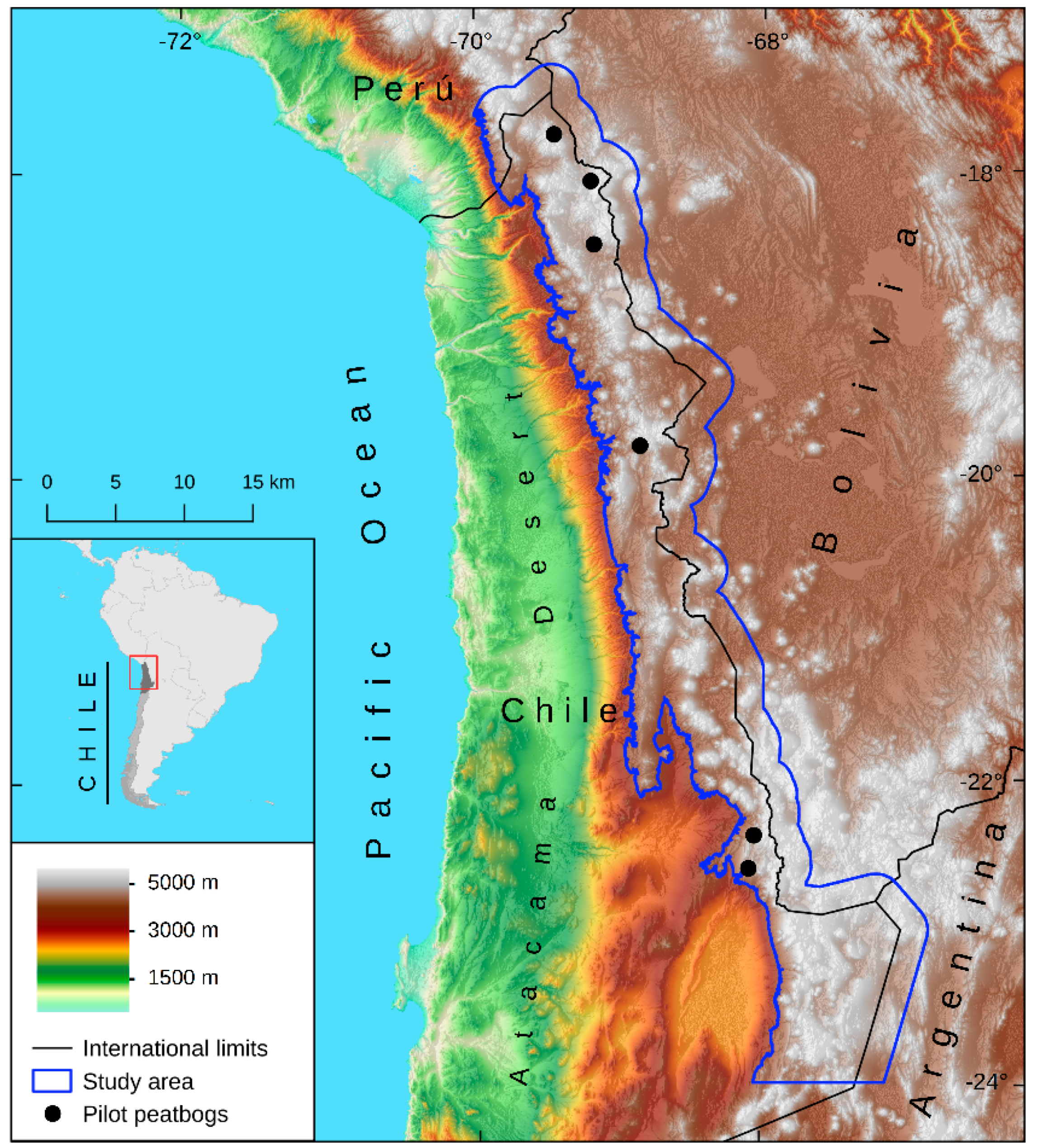
2.3. Preliminary Extent Assessment of Six Pilot Peatlands
2.4. Large-Scale Digital Inventory of High Andean Peatlands
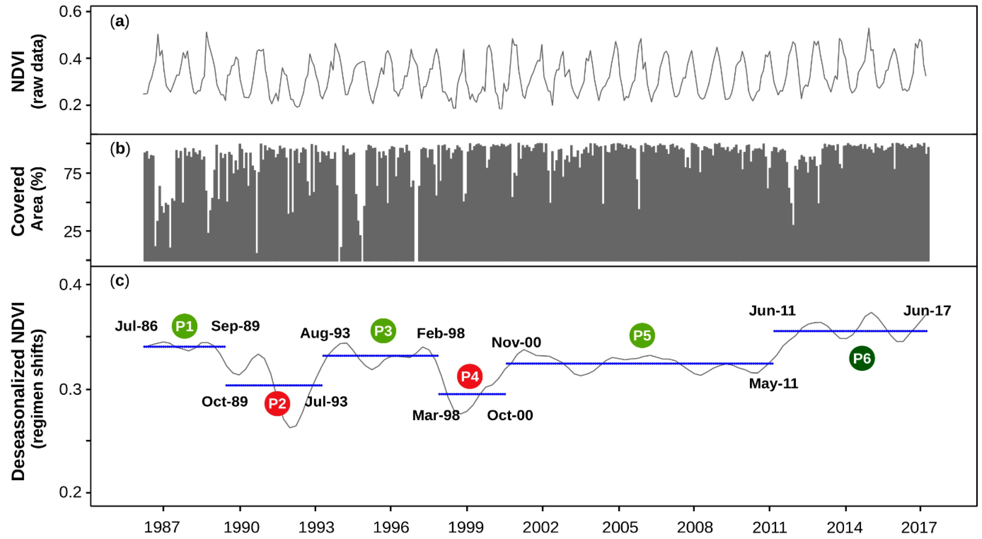
2.5. Time-Series Analysis and Productivity Assessment at Different Spatial Scales
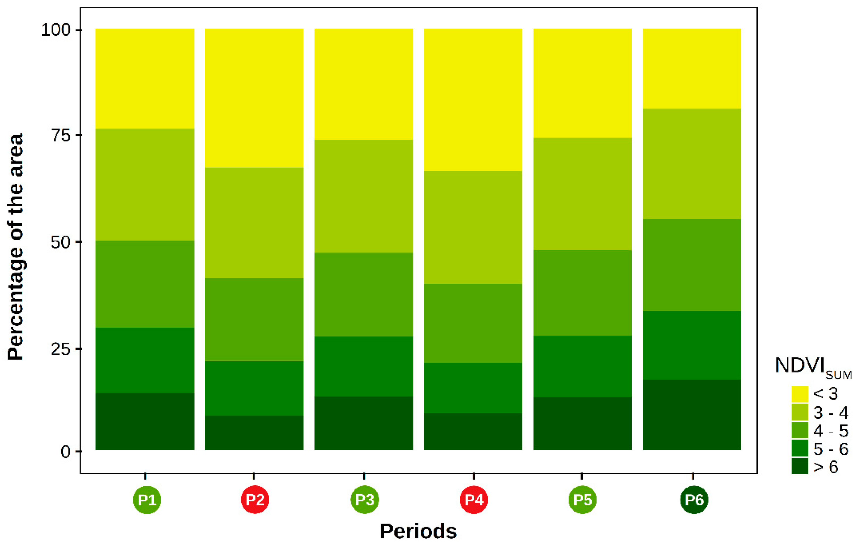
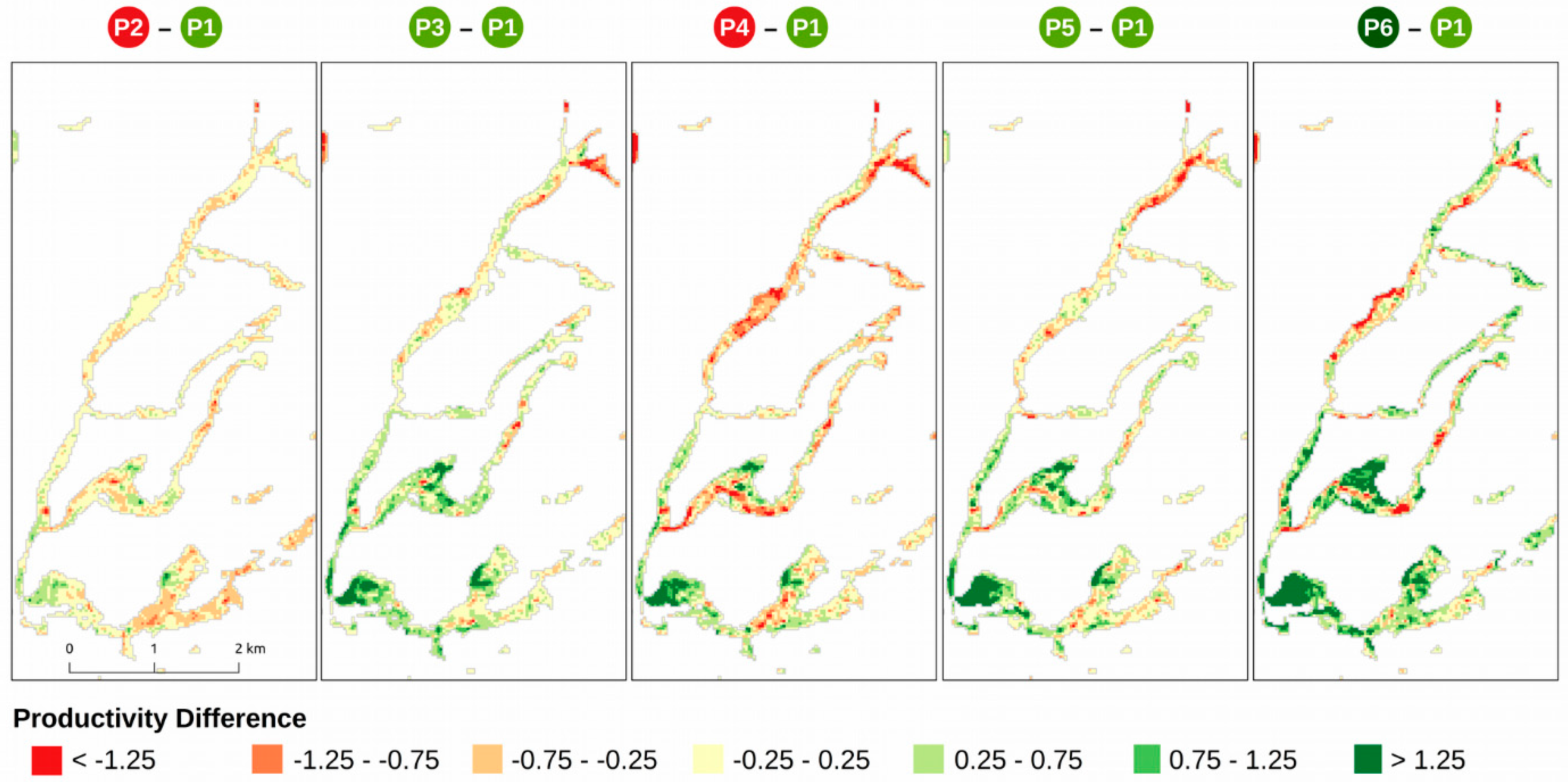
2.6. Spatiotemporal Changes in Productivity
3. Results
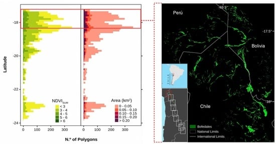
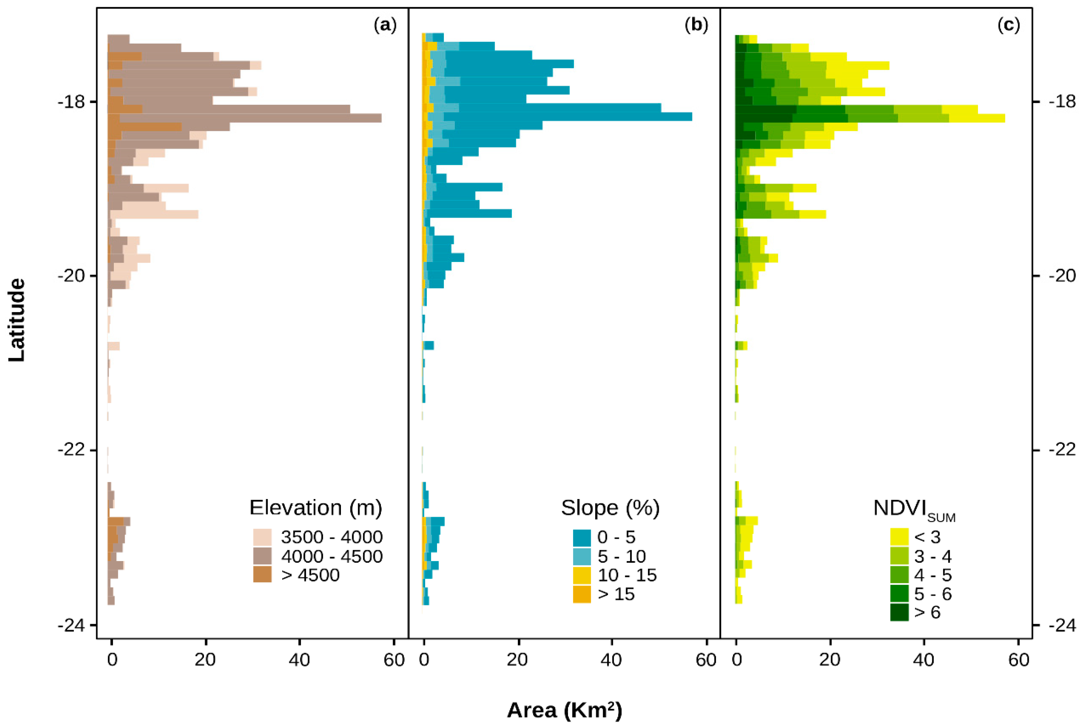
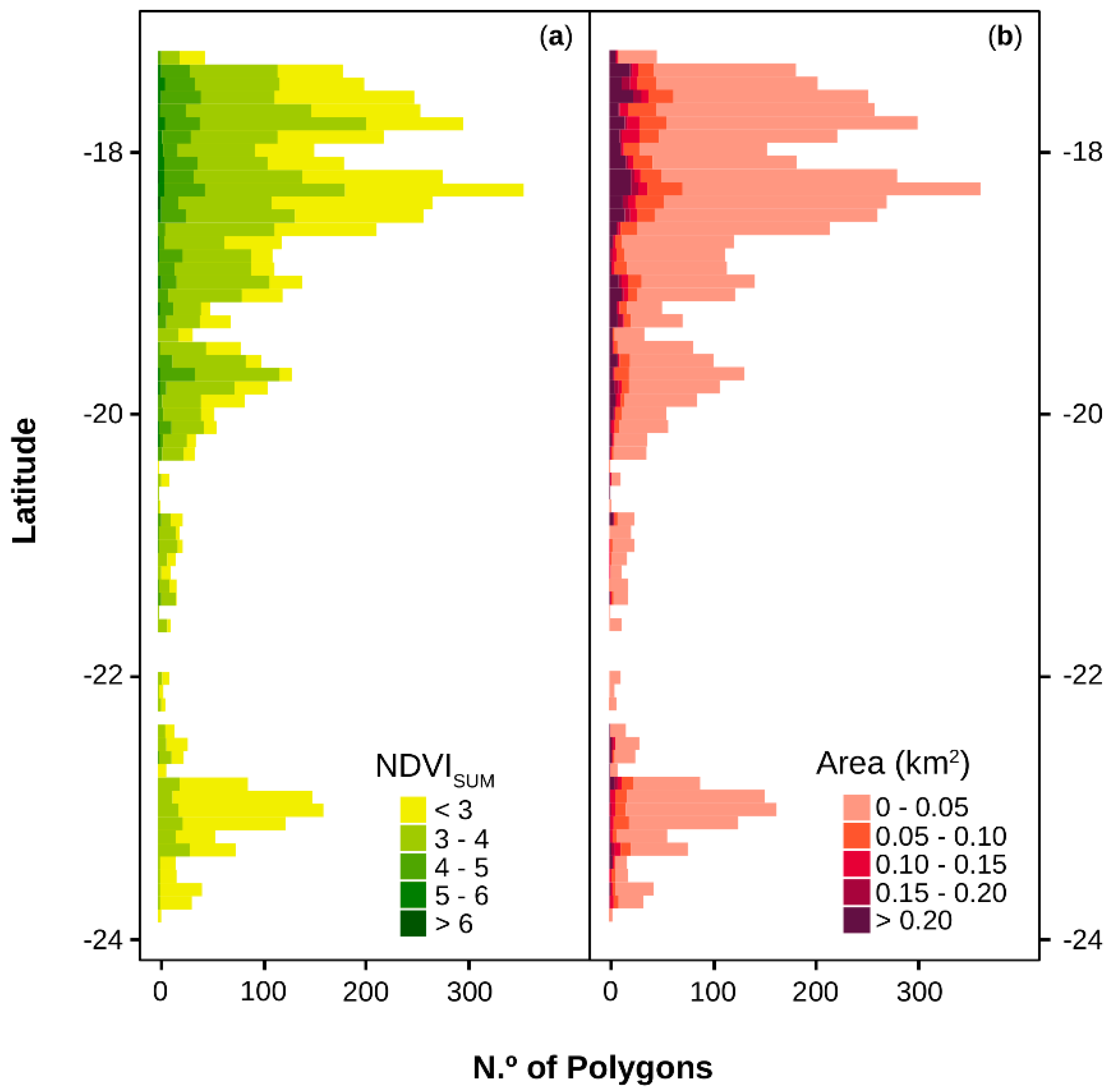
3.1. Digital Inventory of High Andean Peatlands
3.2. Accuracy Assessment of the Digital Inventory
3.3. Multiscale Annual Peatland Productivity Assessment
4. Discussion
5. Conclusions
Supplementary Materials
Author Contributions
Funding
Acknowledgments
Conflicts of Interest
Appendix A


References
- Hu, S.; Niu, Z.; Chen, Y.; Li, L.; Zhang, H. Global wetlands: Potential distribution, wetland loss, and status. Sci. Total Environ. 2017, 586, 319–327. [Google Scholar] [CrossRef] [PubMed]
- Lehner, B.; Döll, P. Development and validation of a global database of lakes, reservoirs and wetlands. J. Hydrol. 2004, 296, 1–22. [Google Scholar] [CrossRef]
- Mitsch, W.J.; Gosselink, J.G. Wetlands of the world. In Wetlands; John Wiley & Sons, Inc.: Hoboken, NJ, USA, 2015; pp. 45–110. [Google Scholar]
- Minasny, B.; Berglund, Ö.; Connolly, J.; Hedley, C.; de Vries, F.; Gimona, A.; Kempen, B.; Kidd, D.; Lilja, H.; Malone, B.; et al. Digital mapping of peatlands—A critical review. Earth-Sci. Rev. 2019, 196, 102870. [Google Scholar] [CrossRef]
- Yu, Z.; Loisel, J.; Brosseau, D.P.; Beilman, D.W.; Hunt, S.J. Global peatland dynamics since the Last Glacial Maximum. Geophys. Res. Lett. 2010, 37. [Google Scholar] [CrossRef]
- Villarroel, E.K.; Mollinedo, P.L.P.; Domic, A.I.; Capriles, J.M.; Espinoza, C. Local Management of Andean Wetlands in Sajama National Park, Bolivia. Mt. Res. Dev. 2014, 34, 356–368. [Google Scholar] [CrossRef]
- Ledru, M.-P.; Jomelli, V.; Bremond, L.; Ortuño, T.; Cruz, P.; Bentaleb, I.; Sylvestre, F.; Kuentz, A.; Beck, S.; Martin, C.; et al. Evidence of moist niches in the Bolivian Andes during the mid-Holocene arid period. Holocene 2013, 23, 1547–1559. [Google Scholar] [CrossRef]
- Yager, K.; Valdivia, C.; Slayback, D.; Jimenez, E.; Meneses, R.I.; Palabral, A.; Bracho, M.; Romero, D.; Hubbard, A.; Pacheco, P.; et al. Socio-ecological dimensions of Andean pastoral landscape change: Bridging traditional ecological knowledge and satellite image analysis in Sajama National Park, Bolivia. Reg. Environ. Chang. 2019, 19, 1353–1369. [Google Scholar] [CrossRef]
- Hribljan, J.A.; Cooper, D.J.; Sueltenfuss, J.; Wolf, E.C.; Heckman, K.A.; Lilleskov, E.; Chimner, R.A. Carbon storage and long-term rate of accumulation in high-altitude Andean peatlands of Bolivia. Mires Peat 2015, 15, 14. [Google Scholar]
- Cooper, D.J.; Kaczynski, K.; Slayback, D.; Yager, K. Growth and Organic Carbon Production in Peatlands Dominated by Distichia muscoides, Bolivia, South America. Arctic Antarct. Alp. Res. 2015, 47, 505–510. [Google Scholar] [CrossRef]
- Earle, L.R.; Warner, B.G.; Aravena, R. Rapid development of an unusual peat-accumulating ecosystem in the Chilean Altiplano. Quat. Res. 2003, 59, 2–11. [Google Scholar] [CrossRef]
- Schittek, K.; Kock, S.T.; Lücke, A.; Hense, J.; Ohlendorf, C.; Kulemeyer, J.J.; Lupo, L.C.; Schäbitz, F. A high-altitude peatland record of environmental changes in the NW Argentine Andes (24 °S) over the last 2100 years. Clim. Past 2016, 12, 1165–1180. [Google Scholar] [CrossRef] [Green Version]
- Engel, Z.; Skrzypek, G.; Chuman, T.; Šefrna, L.; Mihaljevič, M. Climate in the Western Cordillera of the Central Andes over the last 4300 years. Quat. Sci. Rev. 2014, 99, 60–77. [Google Scholar] [CrossRef]
- Kock, S.T.; Schittek, K.; Mächtle, B.; Wissel, H.; Maldonado, A.; Lücke, A. Late Holocene environmental changes reconstructed from stable isotope and geochemical records from a cushion-plant peatland in the Chilean Central Andes (27 °S). J. Quat. Sci. 2019, 34, 153–164. [Google Scholar] [CrossRef] [Green Version]
- Gandarillas, V.; Jiang, Y.; Irvine, K. Assessing the services of high mountain wetlands in tropical Andes: A case study of Caripe wetlands at Bolivian Altiplano. Ecosyst. Serv. 2016, 19, 51–64. [Google Scholar] [CrossRef]
- Moreau, S.; Bosseno, R.; Gu, X.F.; Baret, F. Assessing the biomass dynamics of Andean bofedal and totora high-protein wetland grasses from NOAA/AVHRR. Remote Sens. Environ. 2003, 85, 516–529. [Google Scholar] [CrossRef]
- Neukom, R.; Rohrer, M.; Calanca, P.; Salzmann, N.; Huggel, C.; Acuña, D.; Christie, D.A.; Morales, M.S. Facing unprecedented drying of the Central Andes? Precipitation variability over the period AD 1000-2100. Environ. Res. Lett. 2015, 10, 084017. [Google Scholar] [CrossRef]
- Izquierdo, A.E.; Foguet, J.; Ricardo Grau, H. Mapping and spatial characterization of Argentine High Andean peatbogs. Wetl. Ecol. Manag. 2015, 23, 963–976. [Google Scholar] [CrossRef]
- Casagranda, E.; Navarro, C.; Grau, H.R.; Izquierdo, A.E. Interannual lake fluctuations in the Argentine Puna: Relationships with its associated peatlands and climate change. Reg. Environ. Chang. 2019, 19, 1737–1750. [Google Scholar] [CrossRef]
- García, C.L.; Teich, I.; Gonzalez-Roglich, M.; Kindgard, A.F.; Ravelo, A.C.; Liniger, H. Land degradation assessment in the Argentinean Puna: Comparing expert knowledge with satellite-derived information. Environ. Sci. Policy 2019, 91, 70–80. [Google Scholar] [CrossRef]
- Dangles, O.; Rabatel, A.; Kraemer, M.; Zeballos, G.; Soruco, A.; Jacobsen, D.; Anthelme, F. Ecosystem sentinels for climate change? Evidence of wetland cover changes over the last 30 years in the tropical Andes. PLoS ONE 2017, 12, e0175814. [Google Scholar] [CrossRef] [Green Version]
- Baldassini, P.; Volante, J.N.; Califano, L.M.; Paruelo, J.M. Regional characterization of the structure and productivity of the vegetation of the Puna using MODIS images. Ecol. Austral 2012, 22, 22–32. [Google Scholar]
- Boyle, T.P.; Caziani, S.M.; Waltermire, R.G. Landsat TM inventory and assessment of waterbird habitat in the southern altiplano of South America. Wetl. Ecol. Manag. 2005, 12, 563–573. [Google Scholar] [CrossRef]
- Otto, M.; Scherer, D.; Richters, J. Hydrological differentiation and spatial distribution of high altitude wetlands in a semi-arid Andean region derived from satellite data. Hydrol. Earth Syst. Sci. 2011, 15, 1713–1727. [Google Scholar] [CrossRef] [Green Version]
- Garcia, E.; Otto, M. Caracterización ecohidrológica de humedales alto andinos usando imágenes de satélite multitemporales en la cabecera de cuenca del Río Santa, Ancash, Perú. Ecol. Apl. 2015, 14, 115–125. [Google Scholar] [CrossRef] [Green Version]
- Thibeault, J.; Seth, A.; Wang, G. Mechanisms of summertime precipitation variability in the bolivian altiplano: Present and future. Int. J. Climatol. 2012, 32, 2033–2041. [Google Scholar] [CrossRef]
- Vuille, M.; Bradley, R.S.; Keimig, F. Climate variability in the Andes of Ecuador and its relation to tropical Pacific and Atlantic Sea Surface temperature anomalies. J. Clim. 2000, 13, 2520–2535. [Google Scholar] [CrossRef]
- Minvielle, M.; Garreaud, R.D. Projecting rainfall changes over the South American Altiplano. J. Clim. 2011, 24, 4577–4583. [Google Scholar] [CrossRef]
- Garreaud, R.; Vuille, M.; Clement, A.C. The climate of the Altiplano: Observed current conditions and mechanisms of past changes. Palaeogeogr. Palaeoclimatol. Palaeoecol. 2003, 194, 5–22. [Google Scholar] [CrossRef] [Green Version]
- Vuille, M.; Bradley, R.S.; Keimig, F. Interannual climate variability in the Central Andes and its relation to tropical Pacific and Atlantic forcing. J. Geophys. Res. Atmos. 2000, 105, 12447–12460. [Google Scholar] [CrossRef] [Green Version]
- Squeo, F.A.; Warner, B.; Aravena, R.; Espinoza, D. Bofedales: High altitude peatlands of the central Andes. Rev. Chil. Hist. Nat. 2006, 79, 245–255. [Google Scholar] [CrossRef] [Green Version]
- Ardila, J.P.; Bijker, W.; Tolpekin, V.A.; Stein, A. Context-sensitive extraction of tree crown objects in urban areas using VHR satellite images. Int. J. Appl. Earth Obs. Geoinf. 2012, 15, 57–69. [Google Scholar] [CrossRef] [Green Version]
- Chávez, R.O.; Estay, S.A.; Riquelme, G. npphen. Vegetation Phenological Cycle and Anomaly Detection Using Remote Sensing Data; UACH, PUCV: Valparaíso, Chile, 2017. [Google Scholar]
- Chávez, R.O.; Moreira-Muñoz, A.; Galleguillos, M.; Olea, M.; Aguayo, J.; Latín, A.; Aguilera-Betti, I.; Muñoz, A.A.; Manríquez, H. GIMMS NDVI time series reveal the extent, duration, and intensity of “blooming desert” events in the hyper-arid Atacama Desert, Northern Chile. Int. J. Appl. Earth Obs. Geoinf. 2019, 76, 193–203. [Google Scholar] [CrossRef]
- Bowman, D.M.J.S.; Moreira-Muñoz, A.; Kolden, C.A.; Chávez, R.O.; Muñoz, A.A.; Salinas, F.; González-Reyes, Á.; Rocco, R.; de la Barrera, F.; Williamson, G.J.; et al. Human–environmental drivers and impacts of the globally extreme 2017 Chilean fires. Ambio 2019, 48, 350–362. [Google Scholar] [CrossRef] [PubMed]
- Estay, S.A.; Chávez, R.O.; Rocco, R.; Gutiérrez, A.G. Quantifying massive outbreaks of the defoliator moth Ormiscodes amphimone in deciduous Nothofagus-dominated southern forests using remote sensing time series analysis. J. Appl. Entomol. 2019, 143, 787–796. [Google Scholar] [CrossRef]
- Chávez, R.O.; Rocco, R.; Gutiérrez, Á.G.; Dörner, M.; Estay, S.A. A self-calibrated non-parametric time series analysis approach for assessing insect defoliation of broad-leaved deciduous Nothofagus pumilio forests. Remote Sens. 2019, 11, 204. [Google Scholar] [CrossRef] [Green Version]
- Goward, S.N.; Dye, D.G. Evaluating North American net primary productivity with satellite observations. Adv. Sp. Res. 1987, 7, 165–174. [Google Scholar] [CrossRef]
- Broich, M.; Huete, A.; Paget, M.; Ma, X.; Tulbure, M.; Coupe, N.R.; Evans, B.; Beringer, J.; Devadas, R.; Davies, K.; et al. A spatially explicit land surface phenology data product for science, monitoring and natural resources management applications. Environ. Model. Softw. 2015, 64, 191–204. [Google Scholar] [CrossRef]
- Cleveland, R.B.; Cleveland, W.S.; McRae, J.E.; Terpenning, I. STL: A seasonal-trend decomposition. J. Off. Stat. 1990, 6, 3–73. [Google Scholar]
- Jamali, S.; Jönsson, P.; Eklundh, L.; Ardö, J.; Seaquist, J. Detecting changes in vegetation trends using time series segmentation. Remote Sens. Environ. 2015, 156, 182–195. [Google Scholar] [CrossRef]
- Rodionov, S.N. A sequential algorithm for testing climate regime shifts. Geophys. Res. Lett. 2004, 31, L09204 1-4. [Google Scholar] [CrossRef] [Green Version]
- Jin, H.; Jönsson, A.M.; Olsson, C.; Lindström, J.; Jönsson, P.; Eklundh, L. New satellite-based estimates show significant trends in spring phenology and complex sensitivities to temperature and precipitation at northern European latitudes. Int. J. Biometeorol. 2019, 63, 763–775. [Google Scholar] [CrossRef] [PubMed] [Green Version]
- Stanfield, R.E.; Dong, X.; Xi, B.; Kennedy, A.; Del Genio, A.D.; Minnis, P.; Jiang, J.H. Assessment of NASA GISS CMIP5 and Post-CMIP5 Simulated Clouds and TOA Radiation Budgets Using Satellite Observations. Part I: Cloud Fraction and Properties. J. Clim. 2014, 27, 4189–4208. [Google Scholar] [CrossRef]
- Drusch, M.; Del Bello, U.; Carlier, S.; Colin, O.; Fernandez, V.; Gascon, F.; Hoersch, B.; Isola, C.; Laberinti, P.; Martimort, P.; et al. Sentinel-2: ESA’s Optical High-Resolution Mission for GMES Operational Services. Remote Sens. Environ. 2012, 120, 25–36. [Google Scholar] [CrossRef]
- Alshammari, L.; Large, J.D.; Boyd, S.D.; Sowter, A.; Anderson, R.; Andersen, R.; Marsh, S. Long-Term Peatland Condition Assessment via Surface Motion Monitoring Using the ISBAS DInSAR Technique over the Flow Country, Scotland. Remote Sens. 2018, 10, 1103. [Google Scholar] [CrossRef] [Green Version]
- Brown, C.; Boyd, S.D.; Sjögersten, S.; Clewley, D.; Evers, L.S.; Aplin, P. Tropical Peatland Vegetation Structure and Biomass: Optimal Exploitation of Airborne Laser Scanning. Remote Sens. 2018, 10, 671. [Google Scholar] [CrossRef] [Green Version]
- Arroyo-Mora, P.J.; Kalacska, M.; Soffer, J.R.; Moore, R.T.; Roulet, T.N.; Juutinen, S.; Ifimov, G.; Leblanc, G.; Inamdar, D. Airborne Hyperspectral Evaluation of Maximum Gross Photosynthesis, Gravimetric Water Content, and CO2 Uptake Efficiency of the Mer Bleue Ombrotrophic Peatland. Remote Sens. 2018, 10, 565. [Google Scholar] [CrossRef] [Green Version]
- McPartland, Y.M.; Falkowski, J.M.; Reinhardt, R.J.; Kane, S.E.; Kolka, R.; Turetsky, R.M.; Douglas, A.T.; Anderson, J.; Edwards, D.J.; Palik, B.; et al. Characterizing Boreal Peatland Plant Composition and Species Diversity with Hyperspectral Remote Sensing. Remote Sens. 2019, 11, 1685. [Google Scholar] [CrossRef] [Green Version]
- Gumbricht, T. Detecting Trends in Wetland Extent from MODIS Derived Soil Moisture Estimates. Remote Sens. 2018, 10, 611. [Google Scholar] [CrossRef] [Green Version]
- Millard, K.; Thompson, K.D.; Parisien, M.-A.; Richardson, M. Soil Moisture Monitoring in a Temperate Peatland Using Multi-Sensor Remote Sensing and Linear Mixed Effects. Remote Sens. 2018, 10, 53. [Google Scholar] [CrossRef] [Green Version]
- Bechtold, M.; Schlaffer, S.; Tiemeyer, B.; De Lannoy, G. Inferring Water Table Depth Dynamics from ENVISAT-ASAR C-Band Backscatter over a Range of Peatlands from Deeply-Drained to Natural Conditions. Remote Sens. 2018, 10, 903. [Google Scholar] [CrossRef] [Green Version]
- Rahman, M.M.; McDermid, G.J.; Strack, M.; Lovitt, J. A New Method to Map Groundwater Table in Peatlands Using Unmanned Aerial Vehicles. Remote Sens. 2017, 9, 1057. [Google Scholar] [CrossRef] [Green Version]
- Kalacska, M.; Arroyo-Mora, P.J.; Soffer, J.R.; Roulet, T.N.; Moore, R.T.; Humphreys, E.; Leblanc, G.; Lucanus, O.; Inamdar, D. Estimating Peatland Water Table Depth and Net Ecosystem Exchange: A Comparison between Satellite and Airborne Imagery. Remote Sens. 2018, 10, 687. [Google Scholar] [CrossRef] [Green Version]
- Asmuß, T.; Bechtold, M.; Tiemeyer, B. On the Potential of Sentinel-1 for High Resolution Monitoring of Water Table Dynamics in Grasslands on Organic Soils. Remote Sens. 2019, 11, 1659. [Google Scholar] [CrossRef] [Green Version]


© 2019 by the authors. Licensee MDPI, Basel, Switzerland. This article is an open access article distributed under the terms and conditions of the Creative Commons Attribution (CC BY) license (http://creativecommons.org/licenses/by/4.0/).
Share and Cite
Chávez, R.O.; Christie, D.A.; Olea, M.; Anderson, T.G. A Multiscale Productivity Assessment of High Andean Peatlands across the Chilean Altiplano Using 31 Years of Landsat Imagery. Remote Sens. 2019, 11, 2955. https://doi.org/10.3390/rs11242955
Chávez RO, Christie DA, Olea M, Anderson TG. A Multiscale Productivity Assessment of High Andean Peatlands across the Chilean Altiplano Using 31 Years of Landsat Imagery. Remote Sensing. 2019; 11(24):2955. https://doi.org/10.3390/rs11242955
Chicago/Turabian StyleChávez, Roberto O., Duncan A. Christie, Matías Olea, and Talia G. Anderson. 2019. "A Multiscale Productivity Assessment of High Andean Peatlands across the Chilean Altiplano Using 31 Years of Landsat Imagery" Remote Sensing 11, no. 24: 2955. https://doi.org/10.3390/rs11242955