A Wide-Adjustable Sensorless IPMSM Speed Drive Based on Current Deviation Detection under Space-Vector Modulation

Abstract

This paper investigates the implementation of a wide-adjustable sensorless interior permanent magnet synchronous motor drive based on current deviation detection under space-vector modulation. A hybrid method that includes a zero voltage vector current deviation and an active voltage vector current deviation under space-vector pulse-width modulation is proposed to determine the rotor position. In addition, the linear transition algorithm between the two current deviation methods is investigated to obtain smooth speed responses at various operational ranges, including at a standstill and at different operating speeds, from 0 to 3000 rpm. A predictive speed-loop controller is proposed to improve the transient, load disturbance, and tracking responses for the sensorless interior permanent magnet synchronous motor (IPMSM) drive system. The computations of the position estimator and control algorithms are implemented by using a digital signal processor (DSP), TMS-320F-2808. Several experimental results are provided to validate the theoretical analysis.

1. Introduction

Interior permanent magnet synchronous motors (IPMSMs) have better performance than any other motors because of their robustness, high efficiency, and high ratio of torque to ampere characteristics [1]. They have been used in industry and household appliances, including machine tools, rolling mills, high-speed trains, electric vehicles, and elevators [2,3]. A sensorless IPMSM drive system can save space, reduce costs, and prevent the noise interference of high-frequency pulse-width modulation (PWM) switching. The major sensorless technologies for an IPMSM include three methods. The first method uses the extended back-electromotive force (back-EMF) estimation to obtain the estimated rotor position [4,5,6,7,8,9]. The extended back-EMF estimation method, however, cannot effectively determine the rotor position at low-speed. The second method uses a high-frequency injection voltage to produce its related high-frequency currents [10,11,12,13,14,15]. The high-frequency injection method, however, requires some extra hardware or software to implement a high-frequency generator and also produces audible noise and electromagnetic interference [10,11,12,13,14,15]. To overcome these issues, the third method uses a stator current deviation to estimate the rotor position. By detecting the current deviation of the stator current, the position estimator has been successfully applied. For example, Bui et al. studied a modified sensorless scheme by using a PWM excitation signal [16]. Wei et al. presented a dual current deviation estimating method to obtain better accuracy of the position estimator [17]. Raute et al. investigated a sensorless technique with the analysis of the inverter nonlinearity effect [18]. Hosogay et al. implemented a position sensorless technique for low-speed ranges based on the d-axis and q-axis current derivative method [19]. These studies have not required any high-frequency injecting signals or a back-EMF estimation [16,17,18,19]. These methods [16,17,18,19], however, have not been applied for all ranges of different speeds.

To solve this problem, a current deviation of the stator current using the active voltage vector (AVV) is developed in [20,21,22,23]. These papers, however, have only focused on middle- to high-speed ranges. In this paper, two novel ideas are proposed as follows:

• a zero voltage vector (ZVV) rotor estimation method is originally proposed to obtain a high-performance sensorless drive system at a zero-speed with full load conditions.
• a linear combination method, including a zero voltage vector (ZVV) algorithm and an AVV algorithm, is proposed with predictive control to operate the sensorless IPMSM drive system from 0 rpm to 3000 rpm. This linear combination method is easily implemented when compared to fuzzy-logic combination methods [24].

2. Mathematical Model of an IPMSM

2.1. The d-q Axis Synchronous Frame Model

According to the rotor flux-linkage coordinate system, the mathematical model of the IPMSM in the d-q axis synchronous frame is expressed as follows:

$$\left[\begin{array}{c}{v}_d\\ v_q\end{array}\right]=\left[\begin{array}{cc}{R}_s+\frac{d}{dt}{L}_d& -{\omega }_e{L}_q\\ {\omega }_e{L}_d& R_s+\frac{d}{dt}{L}_q\end{array}\right]\left[\begin{array}{c}{i}_d\\ i_q\end{array}\right]+\left[\begin{array}{c}0\\ {\omega }_e{\lambda }_m\end{array}\right]$$

(1)

where $v_d$ and $v_q$ are the d-q axis voltages, $R_s$ is the stator resistance, $i_d$ and $i_q$ are the d-q axis currents, $L_d$ and $L_q$ are the d-q axis inductances, ${\omega }_e$ is the electrical rotor speed, and ${\lambda }_m$ is the flux linkage generated by the permanent magnet material, which is placed in the rotor. The addition of the reluctance torque and electromagnetic torque can be obtained as

$$T_e=\frac{3}{2}\frac{P}{2}\left[(L_d-L_q)i_d+{\lambda }_m\right]i_q$$

(2)

The dynamic mechanical equations of the rotor speed and rotor position are expressed as

$$\frac{d}{dt}{\omega }_m=\frac{1}{J_m}(T_e-T_L-B_m{\omega }_m)$$

(3)

and

$$\frac{d}{dt}{\theta }_m={\omega }_m$$

(4)

The electrical rotor position and speed are independently expressed as follows:

$${\theta }_e=\frac{P}{2}{\theta }_m$$

(5)

and

$${\omega }_e=\frac{P}{2}{\omega }_m$$

(6)

where $T_L$ is the external load, $J_m$ is the inertia, $B_m$ is the viscous coefficient, ${\omega }_m$ is the mechanical angular speed, ${\theta }_m$ is the mechanical position, and ${\theta }_e$ is the electrical position.

2.2. The a-b-c Axis Synchronous Frame Model

Considering the three-phase voltage balanced and Y-connected windings of an IPMSM, the a-b-c-axis stator voltage equation can be stated as follows:

$$\left[\begin{array}{c}{v}_{as}\\ v_{bs}\\ v_{cs}\end{array}\right]=\left[\begin{array}{ccc}{r}_a& 0& 0\\ 0& r_b& 0\\ 0& 0& r_c\end{array}\right]\left[\begin{array}{c}{i}_{as}\\ i_{bs}\\ i_{cs}\end{array}\right]+\frac{d}{dt}\left[\begin{array}{c}{\lambda }_{as}\\ {\lambda }_{bs}\\ {\lambda }_{cs}\end{array}\right]$$

(7)

where $v_{as},$ $v_{bs},$ and $v_{cs}$ are the a-, b-, and c-phase voltages, $r_a,$ $r_b,$ and $r_c$ are the a-, b-, and c-phase resistances, and ${\lambda }_{as}$, ${\lambda }_{bs}$, and ${\lambda }_{cs}$ are the a-, b-, and c-phase flux linkages. In Equation (7), the neutral point voltage is assumed to be zero when the neutral point is free because the fundamental components of the $v_{as},$ $v_{bs},$ and $v_{cs}$ are balanced. The relationship between the magnetic flux linkages of three-phase stator windings and the three-phase self-inductances, stator currents, and rotor position can be stated as follows:

$$\left[\begin{array}{c}{\lambda }_{as}\\ {\lambda }_{bs}\\ {\lambda }_{cs}\end{array}\right]=\left[\begin{array}{ccc}{L}_{aa}& M_{ab}& M_{ac}\\ M_{ba}& L_{bb}& M_{bc}\\ M_{ca}& M_{cb}& L_{cc}\end{array}\right]\left[\begin{array}{c}{i}_{as}\\ i_{bs}\\ i_{cs}\end{array}\right]+{\lambda }_m^{}\left[\begin{array}{c}\cos {\theta }_e\\ cos({\theta }_e-\frac{2\pi }{3})\\ cos({\theta }_e+\frac{2\pi }{3})\end{array}\right]$$

(8)

where $L_{aa}$, $L_{bb}$, and $L_{cc}$ are the three-phase self-inductances, and $M_{ab}$, $M_{ac}$, $M_{ba}$, $M_{bc}$, $M_{ca}$, and $M_{cb}$ are the three-phase mutual inductances. The self-inductances are expressed as

$$L_{aa}=L_{ls}+L_{AA}-L_{BB}\cos (2{\theta }_e)$$

(9)

$$L_{bb}=L_{ls}+L_{AA}-L_{BB}\cos (2{\theta }_e+\frac{2\pi }{3})$$

(10)

and

$$L_{cc}=L_{ls}+L_{AA}-L_{BB}\cos (2{\theta }_e-\frac{2\pi }{3})$$

(11)

The mutual inductances are expressed as

$$M_{ab}=M_{ba}==-\frac{1}{2}{L}_{AA}-L_{BB}\cos (2{\theta }_e-\frac{2\pi }{3})$$

(12)

$$M_{bc}=M_{cb}=-\frac{1}{2}{L}_{AA}-L_{BB}\cos (2{\theta }_e)$$

(13)

and

$$M_{ca}=M_{ac}=-\frac{1}{2}{L}_{AA}-L_{BB}\cos (2{\theta }_e+\frac{2\pi }{3})$$

(14)

The $L_{AA}$ and $L_{BB}$ are constant parameters.

3. Zero Voltage Vector-Based Current Deviation Rotor Position Estimator

3.1. Basic Principle

The ZVV dominates the duty cycle of a PWM at a standstill and low-speed operating ranges; as a result, one can substitute $v_d=0$ and $v_q=0$ into Equation (1) and obtain

$$\left[\begin{array}{c}\frac{d{i}_d}{dt}\\ \frac{d{i}_q}{dt}\end{array}\right]=\left[\begin{array}{cc}-\frac{R_s}{L_d}& \frac{L_q}{L_d}{\omega }_e\\ -\frac{L_d}{L_q}{\omega }_e& -\frac{R_s}{L_q}\end{array}\right]\left[\begin{array}{c}{i}_d\\ i_q\end{array}\right]-\left[\begin{array}{c}0\\ \frac{{\lambda }_m{\omega }_e}{L_q}\end{array}\right]$$

(15)

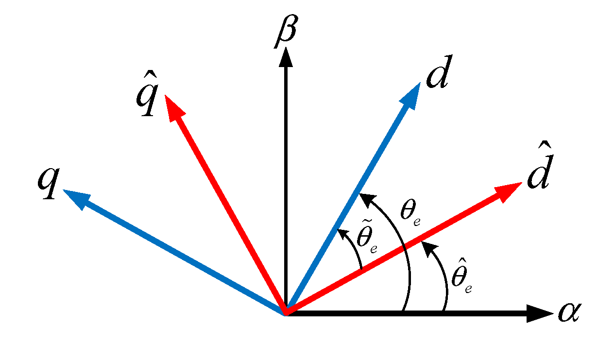
From Figure 1, the estimated position error ${\tilde{\theta }}_e$ is first defined as follows:

$${\tilde{\theta }}_e={\theta }_e-{\widehat{\theta }}_e$$

(16)

where ${\tilde{\theta }}_e$ and ${\widehat{\theta }}_e$ are the estimated rotor position error and estimated rotor position, respectively. Second, the estimated d- and -q axis currents are expressed as follows:

$$\left[\begin{array}{c}{\widehat{i}}_d\\ {\widehat{i}}_q\end{array}\right]=\left[\begin{array}{cc}\cos {\tilde{\theta }}_e& -\sin {\tilde{\theta }}_e\\ \sin {\tilde{\theta }}_e& \cos {\tilde{\theta }}_e\end{array}\right]\left[\begin{array}{c}{i}_d\\ i_q\end{array}\right]=T\left({\tilde{\theta }}_e\right)\left[\begin{array}{c}{i}_d\\ i_q\end{array}\right]$$

(17)

where ${\widehat{i}}_d$ and ${\widehat{i}}_q$ are the estimated d-axis and q-axis currents, and $T({\tilde{\theta }}_e)$ is the coordinate transformation matrix. By substituting Equation (17) into Equation (15), the dynamic equation of the ZVV-based estimated q-axis current is

$$\begin{array}{cc}\frac{d{\widehat{i}}_q}{dt}\cong \hfill & \frac{1}{L_d{L}_q}\left\{R_s\left[\left(L_q-L_d\right){\cos }^2\left({\tilde{\theta }}_e\right)-L_q\right]-\frac{1}{2}{\omega }_e\left(L_q^2-L_d^2\right)\sin \left(2{\tilde{\theta }}_e\right)\right\}{\widehat{i}}_q\hfill \\ \hfill & +\frac{1}{L_d{L}_q}\left\{{\omega }_e\left[\left(L_q^2-L_d^2\right){\cos }^2\left({\tilde{\theta }}_e\right)-L_q^2\right]-\frac{R_s}{2}\left(L_q-L_d\right)\sin \left(2{\tilde{\theta }}_e\right)\right\}{\widehat{i}}_d\hfill \\ \hfill & -\frac{{\lambda }_m{\omega }_e}{L_q}\cos \left({\tilde{\theta }}_e\right)\hfill \end{array}$$

(18)

The values of the $L_d$ and $L_q$ are only a few mHs and are lower than 1 Henry. In consequence, $L_d$ is much greater than $L_d^2$, and $L_q$ is much greater than $L_q^2$. By omitting the $L_d^2$, $L_q^2$, and related items that are multiplied by the ${\omega }_e$, the dynamic equation of the ZVV-based estimated q-axis current can be derived as follows:

$$\begin{array}{cc}\frac{d{\widehat{i}}_q}{dt}\cong \hfill & \frac{R_s}{L_d{L}_q}\{-\left[\left(L_d-L_q\right){\cos }^2\left({\tilde{\theta }}_e\right)+L_q\right]{\widehat{i}}_q\hfill \\ \hfill & +\frac{1}{2}(L_d-L_q)\sin {(2{\tilde{\theta }}_e)}_{}{\widehat{i}}_d\}-\frac{{\lambda }_m{\omega }_e}{L_q}\cos \left({\tilde{\theta }}_e\right)\hfill \end{array}$$

(19)

Because the estimated position error ${\tilde{\theta }}_e$ is close by zero at steady-state, it is feasible to assume that $\sin \left(2{\tilde{\theta }}_e\right)\cong$$2{\tilde{\theta }}_e,$$\sin \left({\tilde{\theta }}_e\right)\cong$${\tilde{\theta }}_e,$${\cos }^2\left({\tilde{\theta }}_e\right)\cong 1$, and $\cos \left({\tilde{\theta }}_e\right)\cong 1$. By using these guestimates into Equation (19), the following equation can be obtained

$$\frac{d{\widehat{i}}_q}{dt}\cong -\frac{R_s{\widehat{i}}_q}{L_q}+\frac{R_s\left(L_d-L_q\right){\widehat{i}}_d}{L_d{L}_q}{\tilde{\theta }}_e-\frac{{\lambda }_m{\omega }_e}{L_q}$$

(20)

3.2. The ZVV Rotor Position Estimating Scheme

In fact, the estimated speed ${\widehat{\omega }}_e$ is employed to replace the real speed ${\omega }_e$. The estimated rotor position ${\tilde{\theta }}_e$ can be assumed to be zero under steady-state conditions. Equation (20), as a result, is rearranged as follows:

$$\frac{d{\widehat{i}}_q}{dt}+\frac{R{\widehat{i}}_q+{\lambda }_m{\widehat{\omega }}_e}{L_q}\cong \frac{R\left(L_d-L_q\right)i_d^{*}}{L_d{L}_q}{\tilde{\theta }}_e$$

(21)

Then, a new variable, $D{\widehat{i}}_q$, can be defined as follows:

$$D{\widehat{i}}_q\triangleq \frac{d{\widehat{i}}_q}{dt}+\frac{R_s{\widehat{i}}_q+{\lambda }_m{\widehat{\omega }}_e}{L_q}$$

(22)

Substituting (22) into Equation (21), one can obtain

$$D{\widehat{i}}_q\cong K_q{\tilde{\theta }}_e$$

(23)

and

$$K_q\triangleq \frac{R_s\left(L_d-L_q\right)i_d^{*}}{L_d{L}_q}$$

(24)

From Equation (23), the $D{\widehat{i}}_q$ is nearly proportional to the estimated position error ${\tilde{\theta }}_e$. Figure 2 illustrates the proposed ZVV-based estimator. First, by using the coordinate transformation, one can transfer the a-, b-, and c-phase current deviations into the estimated d-q axis current deviations. Then, one can derive the current deviation $d{\widehat{i}}_q/dt.$ By summation of the $d{\widehat{i}}_q/dt,$ ${\lambda }_m{\widehat{\omega }}_e/L_q,$ and $R_s{\widehat{i}}_q/L_q,$ one can obtain $D{\widehat{i}}_q.$ Next, one can compute the value of ${\tilde{\theta }}_e$ after dividing $D{\widehat{i}}_q$ by $K_q$ and, thus, obtain the estimated position error. After that, one can use a proportional-integral (PI) controller to acquire the estimated rotor speed and obtain the estimated position by using an integral operation.

4. Active Voltage Vector-Based Current Deviation Rotor Position Estimator

4.1. The AVV Rotor Position Estimation Scheme

At middle and high speeds, the current deviation of the AVV in the a-b-c-stationary frame is used to estimate the position. From Figure 3, when the a-phase upper leg turns on and the b-phase and c-phase lower legs turn on, one can obtain

$$V_{dc}=v_{as}-v_{bs}$$

(25)

By substituting Equation (7) into (25), one can derive

$$V_{dc}=r_s{i}_{as}+\frac{d{\lambda }_a}{dt}-r_s{i}_{bs}-\frac{d{\lambda }_b}{dt}$$

(26)

Substituting Equation (8) into (26), one can derive

$$\begin{array}{c}{V}_{dc}=r_s{i}_{as}+\frac{d}{dt}(L_{aa}{i}_{as}+L_{ab}{i}_{bs}+L_{ac}{i}_{cs}+{\lambda }_m^{}\cos {\theta }_e)-r_s{i}_{bs}\\ -\frac{d}{dt}(L_{ba}{i}_{as}+L_{bb}{i}_{bs}+L_{bc}{i}_{cs}+{\lambda }_m^{}\cos ({\theta }_e-\frac{2\pi }{3}))\end{array}$$

(27)

By substituting Equations (9)–(14) into Equation (27) and doing some mathematical processes, one can obtain

$$\begin{array}{cc}{V}_{dc}=\hfill & [\left(\frac{1}{2}\left(3L_{AA}+2L_{ls}\right)+\sqrt{3}\sin (2{\theta }_e-\frac{\pi }{3})L_{BB}\right)\frac{d{i}_{as}}{dt}+\left(-\frac{1}{2}\left(3L_{AA}+2L_{ls}\right)+\sqrt{3}\sin \left(2{\theta }_e+\pi \right)L_{BB}\right)\frac{d{i}_{bs}}{dt} \hfill \\ \hfill & +\left(\sqrt{3}\sin (2{\theta }_e+\frac{\pi }{3})L_{BB}\right)\frac{d{i}_{cs}}{dt}]+2\sqrt{3}{\omega }_e{L}_{BB}\left[\sin (2{\theta }_e+\frac{\pi }{6})i_{as}+\sin (2{\theta }_e-\frac{\pi }{2})i_{bs}+\sin (2{\theta }_e+\frac{5\pi }{6})i_{cs}\right]\hfill \\ \hfill & -{\lambda }_m{\omega }_e(\frac{3}{2}\sin {\theta }_e+\frac{\sqrt{3}}{2}\cos {\theta }_e)+r_s(i_{as}-i_{bs})\hfill \end{array}$$

(28)

In addition, from Figure 3, when the a-phase upper leg turns on and the b-phase and c-phase lower legs turn on, one can obtain the voltage between the b-phase and c-phase as follows:

$$0 = v_{bs}-v_{cs}$$

(29)

By using the similar processes shown in Equations (26)–(29), one can derive

$$\begin{array}{l}0 =[\left(\sqrt{3}\sin \left(2{\theta }_e+\pi \right)L_{BB}\right)\frac{d{i}_{as}}{dt}+\left(\frac{1}{2}\left(3L_{AA}+2L_{ls}\right)+\sqrt{3}\sin (2{\theta }_e+\frac{\pi }{3})L_{BB}\right)\frac{d{i}_{bs}}{dt}+\left(-\frac{1}{2}\left(3L_{AA}+2L_{ls}\right)+\sqrt{3}\sin (2{\theta }_e-\frac{\pi }{3})L_{BB}\right)\frac{d{i}_{cs}}{dt}]\\ +2\sqrt{3}{\omega }_e{L}_{BB}\left[\sin (2{\theta }_e-\frac{\pi }{2})i_{as}+\sin (2{\theta }_e+\frac{5\pi }{6})i_{bs}+\sin (2{\theta }_e+\frac{\pi }{6})i_{cs}\right]+\sqrt{3}{\lambda }_m{\omega }_e\cos {\theta }_e+r_s(i_{bs}-i_{cs})\end{array}$$

(30)

Moreover, from Figure 3, when the a-phase upper leg turns on and the b-phase and c-phase lower legs turn on, one can obtain

$$i_{as}=-(i_{bs}+i_{cs})$$

(31)

Taking the differential of both sides in Equation (31), one can obtain

$$\frac{d{i}_{as}}{dt}=-(\frac{d{i}_{bs}}{dt}+\frac{d{i}_{cs}}{dt})$$

(32)

From Equations (28), (30), and (32), one can obtain the following equation:

$$\begin{array}{cc}{\frac{d{i}_{as}}{dt}}_{\_mode A+}=\hfill & \{4V_{dc}\left(\frac{2}{3}{L}_{ls}+L_{AA}+L_{BB}\cos \left(2{\theta }_e\right)\right)+2{\omega }_e{L}_{BB}\hfill \\ \hfill & [\left(-3i_{as}\sin \left(2{\theta }_e\right)+\sqrt{3}\left(i_{bs}-i_{cs}\right)\left(3L_{BB}+\cos \left(2{\theta }_e\right)\right)\right)\hfill \\ \hfill & \left(3L_{AA}+2L_{ls}\right)+K_a]+R_{sa}\}/\left[\left(2L_{ls}+3L_{\Delta }\right)\left(2L_{ls}+3L_{\Sigma }\right)\right]\hfill \end{array}$$

(33)

where

$$L_{\Delta }=L_{AA}-L_{BB}$$

(34)

and

$$L_{\Sigma }=L_{AA}+L_{BB}$$

(35)

When the switching state of the inverter is at a zero voltage state, the motor short circuits. Consequently, the direct-current (DC) voltage $V_{dc}$ is equal to zero. By substituting $V_{dc}$ = 0 into Equation (33), one can obtain

$$\begin{array}{cc}{\frac{d{i}_{as}}{dt}}_{\_\mathrm{mode} 0}=\hfill & \{2{\omega }_e{L}_{BB}[\left(-3i_{as}\sin \left(2{\theta }_e\right)+\sqrt{3}\left(i_{bs}-i_{cs}\right)\left(3L_{BB}+\cos \left(2{\theta }_e\right)\right)\right)\hfill \\ \hfill & \left(3L_{AA}+2L_{ls}\right)+K_a]+R_{sa}\}/\left[\left(2L_{ls}+3L_{\Delta }\right)\left(2L_{ls}+3L_{\Sigma }\right)\right]\hfill \end{array}$$

(36)

From Equation (36), the current deviation $d{i}_{as}/dt{\_}_{\mathrm{mode} 0}$ includes a resistance influencing part, a back-EMF influencing part, and an inductance influencing part. To eject the influences of the back-EMF and resistance parts, the a-phase compensated current deviation $D{i}_{as}{}_{\_\mathrm{mode} \mathrm{A}+}$ is computed as

$$\begin{array}{cc}D{i}_{as}{}_{\_\mathrm{mode} \mathrm{A}+}\hfill & ={\frac{d{i}_{as}}{dt}}_{\_\mathrm{mode} \mathrm{A}+}-{\frac{d{i}_{as}}{dt}}_{\_\mathrm{mode} 0}\hfill \\ \hfill & =\frac{4V_{dc}\left[\frac{2}{3}{L}_{ls}+L_{AA}+L_{BB}\cos (2{\theta }_e)\right]}{\left(2L_{ls}+3L_{\Delta }\right)\left(2L_{ls}+3L_{\Sigma }\right)}\hfill \end{array}$$

(37)

From Equation (37), one can observe that the $D{i}_{as}{}_{\_\mathrm{mode} \mathrm{A}+}$ is only related to the inductance and input DC voltage $V_{dc}.$ By using a similar method, one can derive the b-phase compensation current deviation and the c-phase compensation current deviation.

By transferring the a-, b-, and c-axis current deviations into the $\alpha -$ and $\beta -$ axis current-deviations, one can obtain the current deviation $D{i}_{\alpha }$ and $D{i}_{\beta }$ as follows:

$$\left[\begin{array}{c}D{i}_{\alpha }\\ D{i}_{\beta }\end{array}\right]=\left[\begin{array}{ccc}1& -\frac{1}{2}& -\frac{1}{2}\\ 0& \frac{\sqrt{3}}{2}& -\frac{\sqrt{3}}{2}\end{array}\right]\left[\begin{array}{c}D{i}_{as}{}_{\_\mathrm{mode} \mathrm{A}+}\\ D{i}_{bs}{}_{\_\mathrm{mode} \mathrm{B}+}\\ D{i}_{cs}{}_{\_\mathrm{mode} \mathrm{C}+}\end{array}\right]$$

(38)

By substituting the a-b-c-phase compensated current deviation into Equation (38), the $D{i}_{\alpha }$ can be simplified as

$$D{i}_{\alpha }=\frac{6V_{dc}{L}_B\cos (2{\theta }_e)}{\left(2L_{ls}+3L_{\Delta }\right)\left(2L_{ls}+3L_{\Sigma }\right)}$$

(39)

and the $D{i}_{\beta }$ can be simplified as

$$D{i}_{\beta }=\frac{-6V_{dc}{L}_B\sin (2{\theta }_e)}{\left(2L_{ls}+3L_{\Delta }\right)\left(2L_{ls}+3L_{\Sigma }\right)}$$

(40)

By using the following ${\tan }^{-1}$ mathematical process, one can obtain the AVV-based estimated electrical rotor position as follows:

$${\tan }^{-1}(\frac{-D{i}_{\beta }}{D{i}_{\alpha }})=2{\theta }_e$$

(41)

4.2. Space-Vector Extension And Compensation

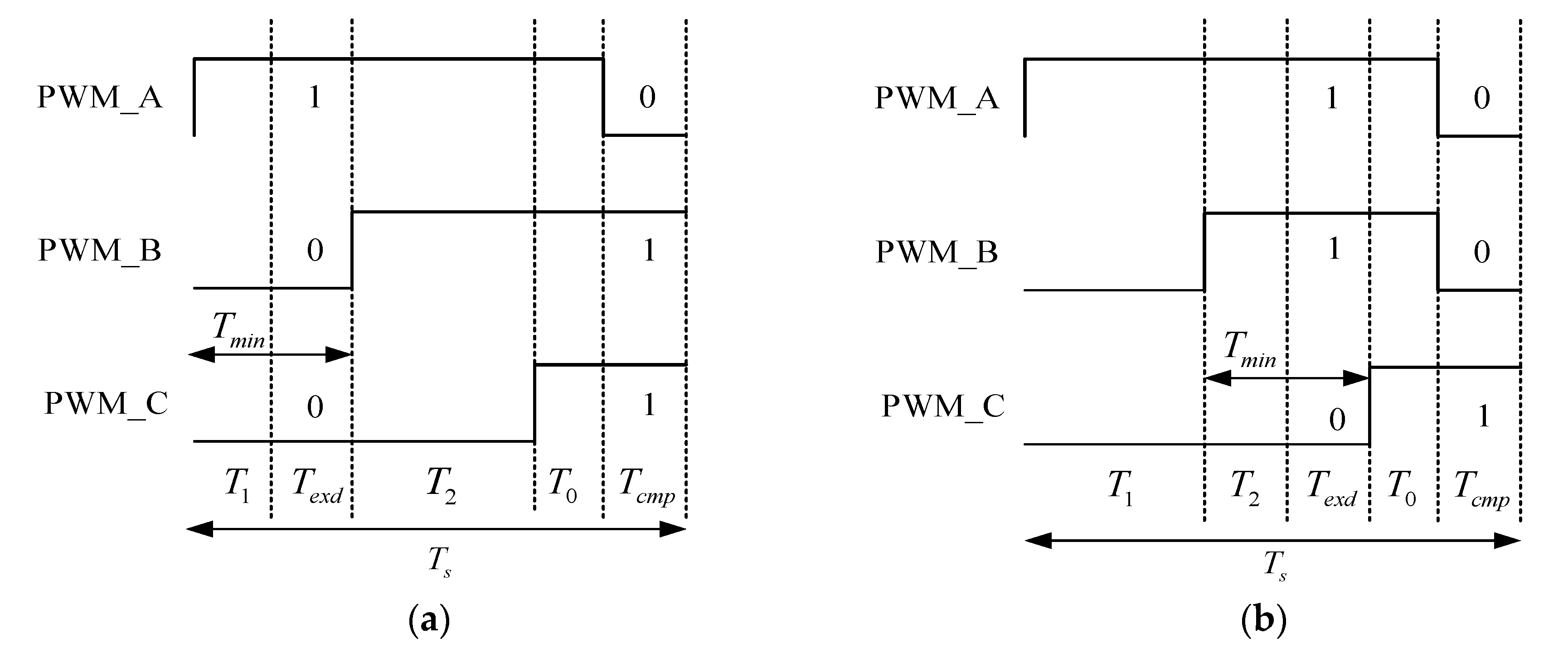
The current deviation is used to estimate the position and is discussed in this section. To obtain the current deviation, two different currents are sampled for each switching state, and then the current deviation can be computed. In the real world, the time interval between the two-sampling intervals should be large enough to obtain an accurate current deviation. However, some turn-on or turn-off intervals are reduced as the motor speed increases. In addition, the switching interval is also varied when the voltage vector moves to different positions. To solve this issue, an extension with a compensation method is used [13]. When the digital signal processor (DSP) detects that the time interval of the switching state is too short, an extension time is automatically provided to make the switching time maintain a minimum required switching time, $T_{\min }.$ In this paper, the minimum required switching time interval $T_{\min }$ is set as 20 μs.

However, the extension time of the switching state causes DC bias and harmonics. Therefore, a compensation time of the whole switching interval is required. Figure 4a,b show the space-vector pulse width modulation (SVPWM) switching states used in this paper. In each switching interval, which is 100 μs, three switching states are generated. Figure 4a shows the $T_1$ switching state when it is too short. When this occurs, the switching state “100” is extended, and its complementary state “011” is compensated for at the end because the voltage in the whole-time interval $T_s$ should be balanced. As a result, the DC bias is reduced to zero, and the ac harmonics are compensated. Figure 4b shows the $T_2$ switching state when it is too short. When this occurs, the switching state “110” is extended. Then, “001” is compensated for at the end of the entire switching interval $T_s$.

5. Current Deviation Detection Technique

In this paper, the current deviation is used to estimate the position of IPMSM. As a result, the precise detection of the current deviation at AVV and ZVV is very important. As one can observe in the waveform, shown in Figure 5, the current deviation is obtained for every sampling time, $T_s$. The current spike can be avoided by carefully selecting the sampling instance. The first current sampling instance of each switching state is delayed 10 μs after the power device turns on. The second current sampling instance is 5 μs before the next switching state occurs. After that, the current deviation can be computed by subtracting the second captured current with the first captured current over the time difference.

The current deviation can be precisely obtained since the time period of AVV is extended if it is too narrow when the motor is operated at middle- and high-speeds. The current-deviation of the ZVV can be obtained because of the large duty cycle of the ZVV when the motor is operated at a standstill and low-speed ranges.

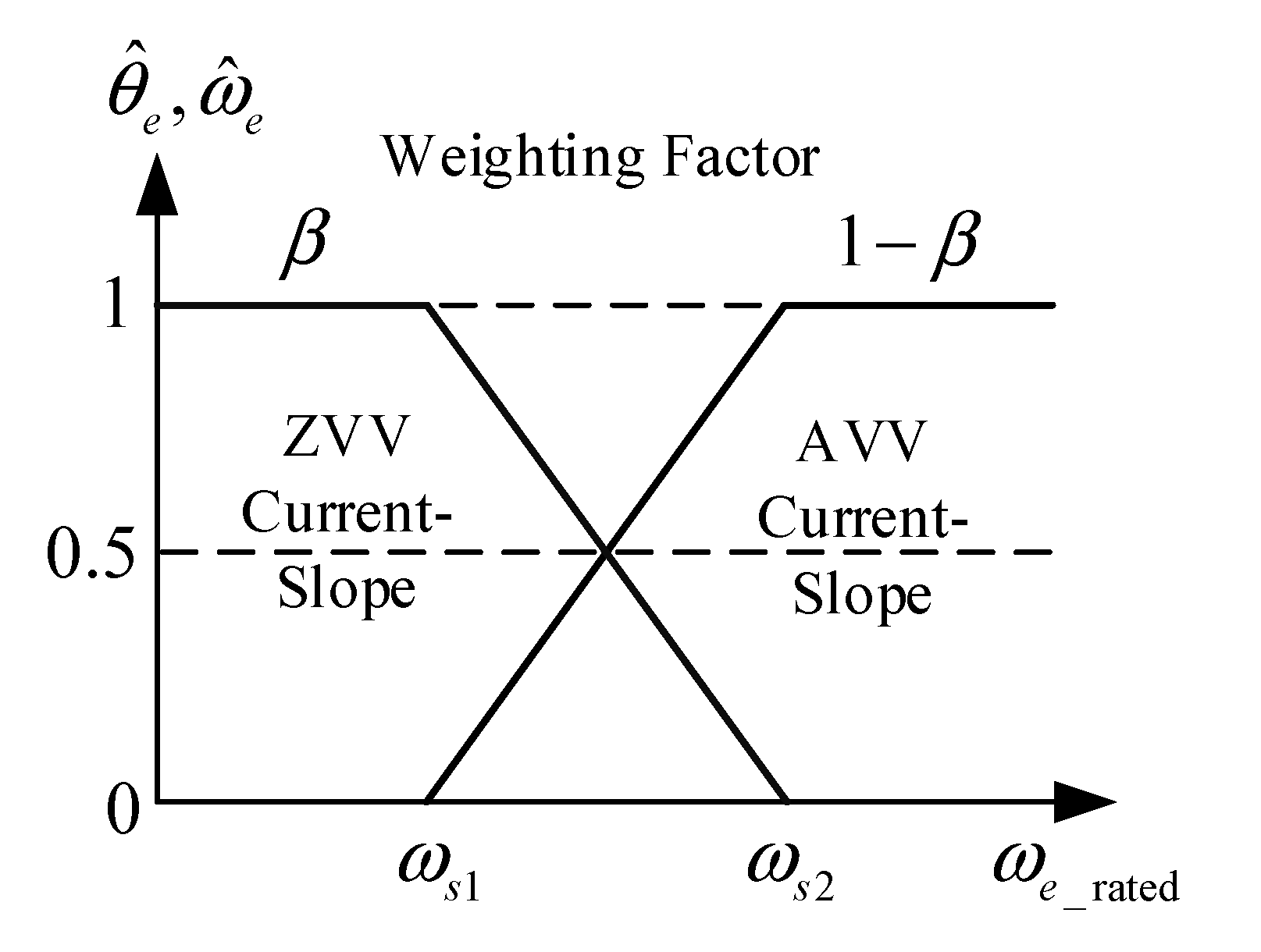
6. Linear Transition from Standstill and Low-Speed to High-Speed

A linear transferring method between the ZVV and AVV algorithms is displayed in Figure 6. This linear transition method is easy to implement and can achieve better performance than other advanced transition methods, such as fuzzy logic methods. Even though fuzzy logic methods have better performance and faster responses, they need more complex computations [24]. A lower bound transition speed, which is 60 rpm, is defined as ${\omega }_{s1}$. In addition, a higher bound transition speed, which is 100 rpm, is defined as ${\omega }_{s2}$. A weighting factor $\beta$ is utilized in the subsequent equations:

$${\widehat{\theta }}_e=\beta {\widehat{\theta }}_{zvv}+\left(1-\beta \right){\widehat{\theta }}_{avv}$$

(42)

and

$${\widehat{\omega }}_e=\beta {\widehat{\omega }}_{zvv}+\left(1-\beta \right){\widehat{\omega }}_{avv}$$

(43)

The weighting factor $\beta$ in (42) and (43) is defined as follows:

$$\beta =\{\begin{array}{l}1\\ \frac{{\omega }_{s2}-{\widehat{\omega }}_e}{{\omega }_{s2}-{\omega }_{s1}}\\ 0\end{array}\begin{array}{l},\mathrm{when} {\widehat{\omega }}_e\le {\omega }_{s1 }\\ , \mathrm{when} {\omega }_{s1 }<{\widehat{\omega }}_e<{\omega }_{s2}\\ ,\mathrm{when} {\widehat{\omega }}_e\ge {\omega }_{s2} \end{array}$$

(44)

where ${\widehat{\theta }}_{zvv}$ and ${\widehat{\theta }}_{avv}$ are the estimated positions by using the ZVV and the AVV algorithms, respectively. The $\widehat{\omega }{ }_{zvv}$ and $\widehat{\omega }{ }_{avv}$ are the estimated speeds after using the ZVV and AVV algorithms. By using this method, the estimated positions and estimated speeds can be accurately obtained.

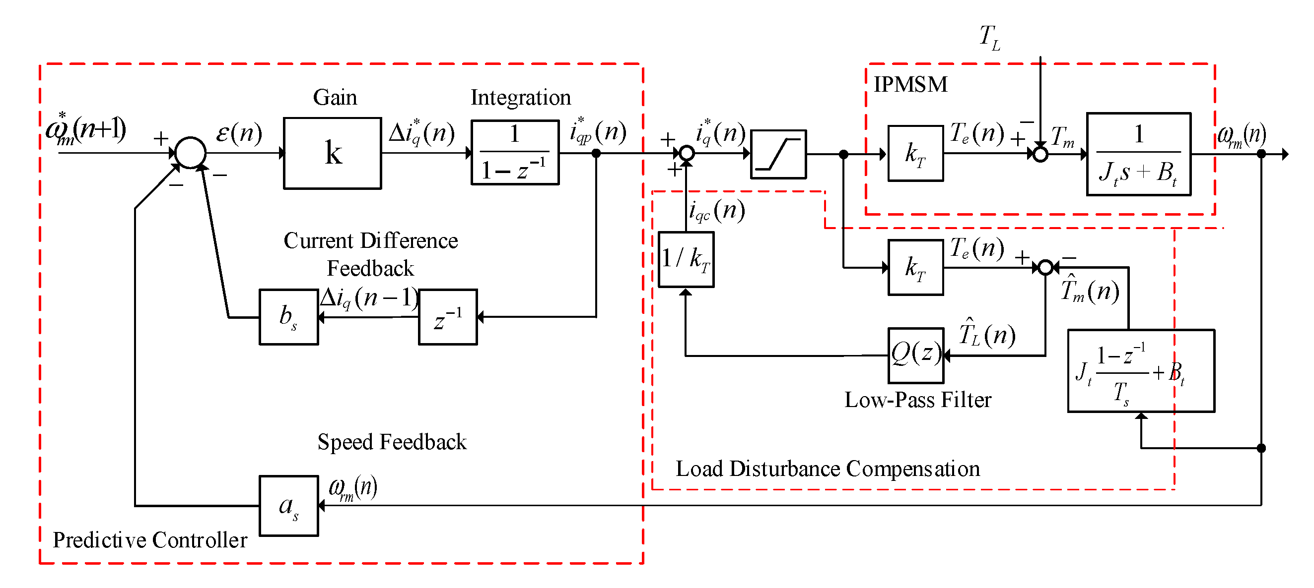
7. Predictive Speed Controller Design

Predictive controllers have been applied in chemical process industries, robotic controls, and other multivariable systems [25,26,27]. Recently, predictive controllers have been successfully employed in motor drives and power electronics [28,29,30]. A predictive speed controller is designed to improve the responses of the drive systems. By omitting the external load $T_L$ from (3), when the d-axis is zero, it is possible to derive the transfer function $G_p(s)$ of the IPMSM, which is shown in Figure 7, as follows:

$$G_p(s)=\frac{{\omega }_m(s)}{i_q(s)}=\frac{K_t/J_t}{s+(B_t/J_t)}$$

(45)

By inserting a zero-order hold device and taking the z-transformation, one can obtain

$$G_p(z)=\frac{{\omega }_m(z)}{i_q(z)}=\frac{K_t}{B_t}\frac{(1-e^{-\frac{B_t}{J_t}{T}_s})}{(z-e^{-\frac{B_t}{J_t}{T}_s})}$$

(46)

From (46), it is straightforward to derive the speed prediction as

$${\omega }_m(n+1)=a_s{\omega }_m(n)+b_s{i}_q(n)$$

(47)

where

$$a_s=e^{-\frac{B_t}{J_t}{T}_s}$$

(48)

and

$$b_s=\frac{K_t}{B_t}(1-e^{-\frac{B_t}{J_t}{T}_s})$$

(49)

The predictive speed equation is shown as

$$\begin{array}{l}{\stackrel{⌢}{\omega }}_m(n+1)=a_s{\omega }_m(n)+b_s{i}_{qp}{}^{*}(n)\\ =a_s{\omega }_m(n)+b_s{i}_{qp}(n-1)+b_s\Delta i_q{}^{*}(n)\end{array}$$

(50)

The performance index can be defined as [28,29,30]

$$J_p(n)=\alpha {\left[{\stackrel{⌢}{\omega }}_m(n+1)-{\omega }_m{}^{*}(n+1)\right]}^2+{\left[\Delta i_q{}^{*}(n)\right]}^2$$

(51)

After taking $\partial J_p(n)/\partial \Delta i_q{}^{*}(n)=0$, one can obtain

$$2\alpha b_s\left[a_s{\omega }_m(n)+b_s\left(i_{qp}(n-1)+\Delta i_q{}^{*}(n)\right)-{\omega }_m{}^{*}(n+1)\right]+2\Delta i_q{}^{*}(n)=0$$

(52)

Next, one can obtain

$$\Delta i_q{}^{*}(n)=\frac{\alpha b_s}{\alpha b_s{}^2+1}\left[{\omega }_m{}^{*}(n+1)-a_s{\omega }_m(n)-b_s{i}_{qp}(n-1)\right]$$

(53)

and

$$k=\frac{\alpha b_s}{\alpha b_s{}^2+1}$$

(54)

Finally, the q-axis current command is

$$i_{qp}{}^{*}(n)=i_{qp}(n-1)+\Delta i_q{}^{*}(n)$$

(55)

Load disturbance compensation is shown in Figure 7. By computing the difference between $k_t{i}_q^{*}(n)$ and $J_t(\Delta {\omega }_m/\Delta t)+B_t{\omega }_m$, the estimated mechanical load can be obtained. Next, the external load ${\widehat{T}}_m(n)$ is estimated by using a low-pass filter. After that, the compensation current $i_{qc}(n)$ can be obtained. Finally, the q-axis current command $i_q{}^{*}(n)$, which is the summation of the $i_{qp}{}^{*}(n)$ and the compensation current $i_{qc}(n)$, can be computed, shown in Figure 7.

8. Implementation

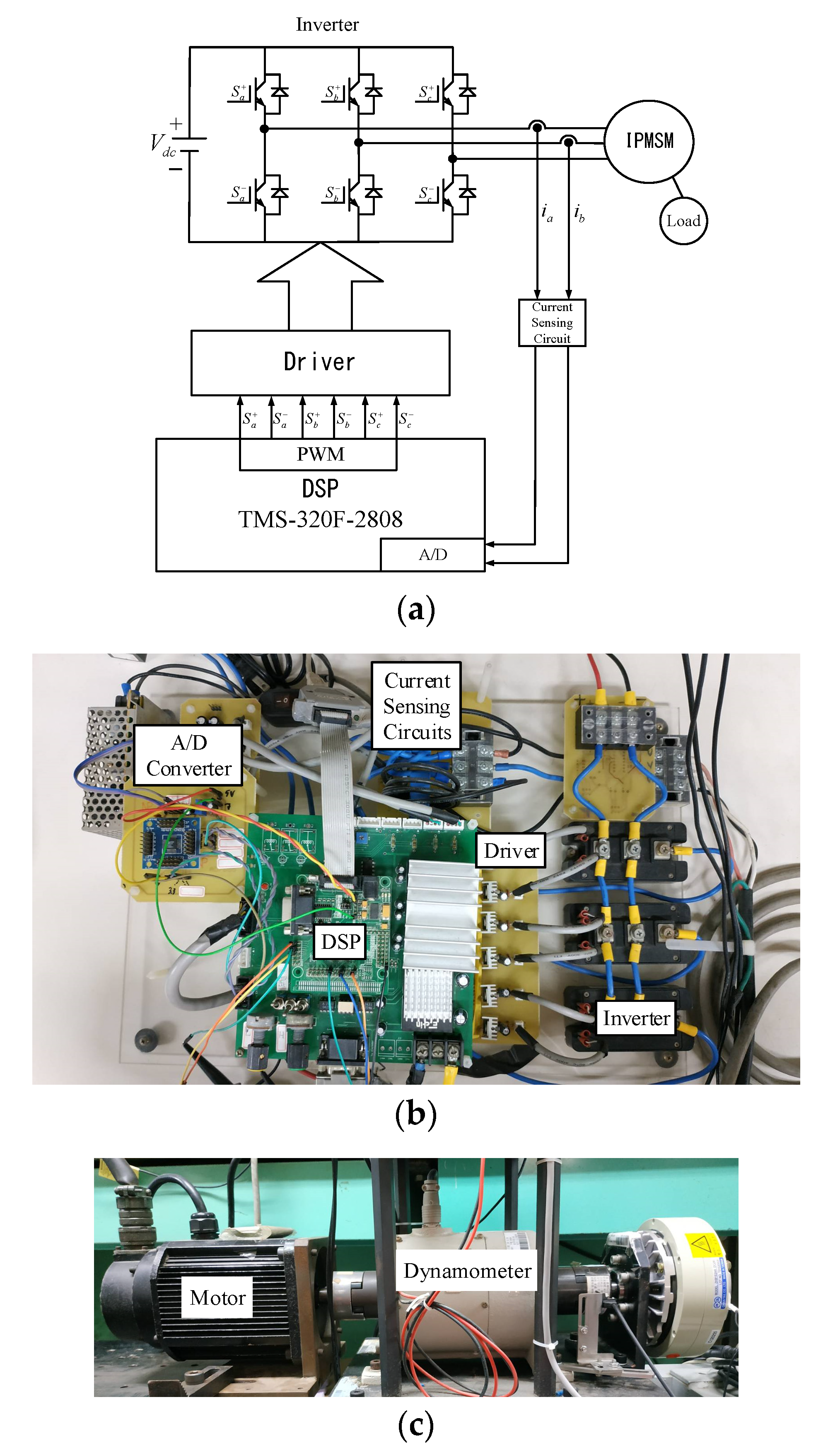
The implemented circuit of the sensorless IPMSM drive system is discussed here. Figure 8a demonstrates the closed-loop block diagram of the implemented drive system. The digital signal processor (DSP) executes the position estimation and predictive control algorithms. As a result, the DSP is the control center of the IPMSM drive system. Figure 8b displays the implemented circuit, including an inverter, a 3-phase driving circuit, a DSP, two A/D converters, and two Hall-effect current sensing circuits. Figure 8c demonstrates the drive system with a dynamometer, which is driven by a DC permanent magnet motor to equip the external load. By suitably adjusting the input voltage of the DC motor, a varied load can be obtained. The IPMSM is an 8-pole, 7.7 A, 2000 rpm, 2 kW IPMSM. The motor has the following parameters: stator resistance = 0.32 Ω, d-axis self-inductance = 0.0049 H, q-axis self-inductance = 0.0078 H, flux linkage = 0.16 V.s/rad, inertia = 0.00455 kg-m${}^2,$ viscous coefficient = 0.003 N.m.s/rad, switching frequency of the inverter = 10 kHz, DC bus voltage = 300 V, current-loop sampling interval = 100 μs, and the speed-loop sampling interval = 1 ms.

9. Experimental Results

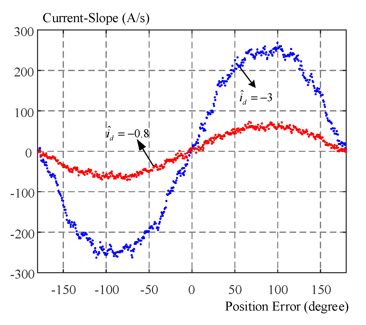
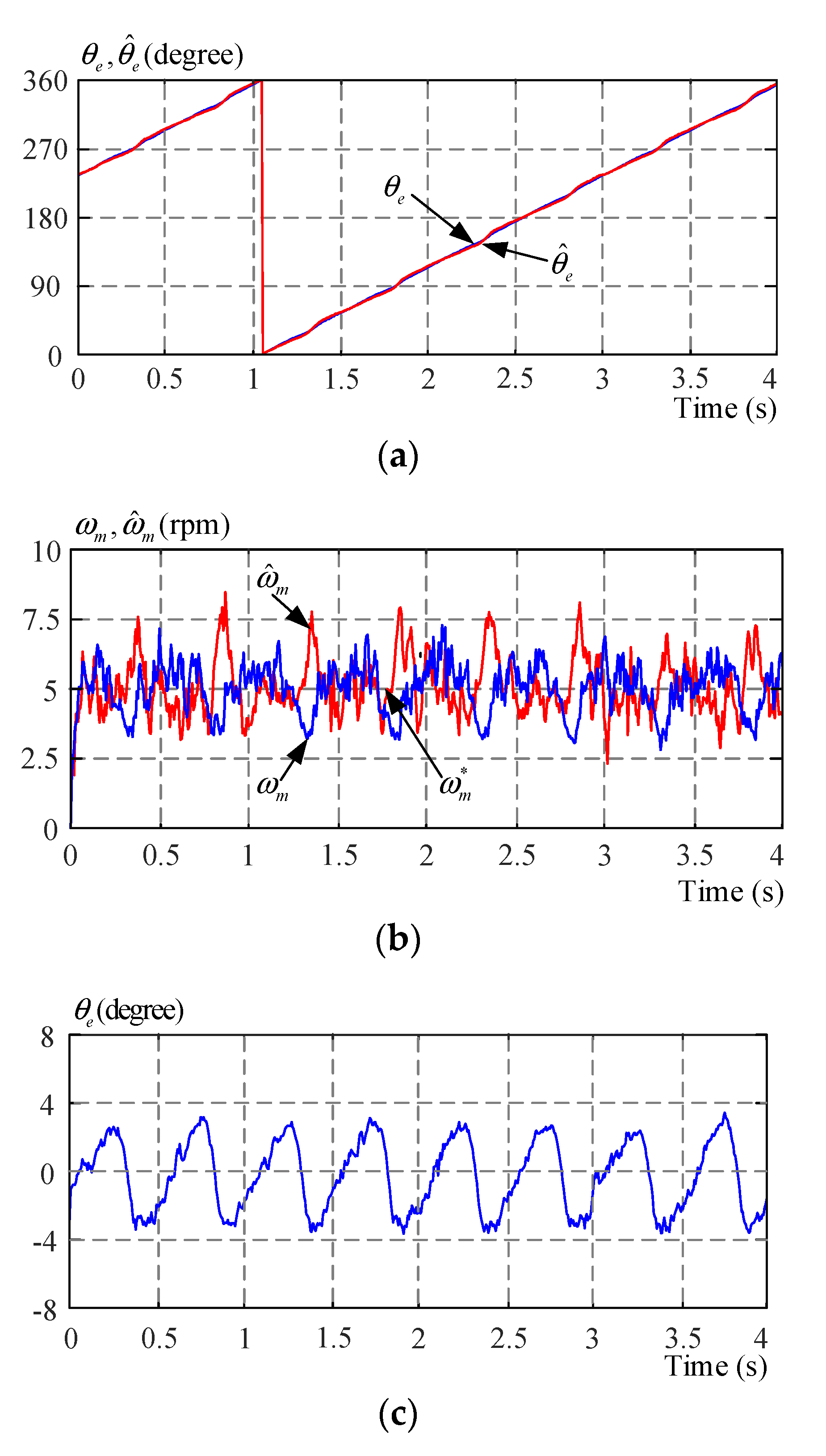
To verify the theoretical analysis, several measured results are demonstrated in this section. The speed-loop PI controller is designed by a pole assignment technique. Figure 9 demonstrates the relation between the q-axis current deviations and estimated position errors at 0 rpm. When the d-axis current is too low, the amplitude of the q-axis current deviation is also very low. In order to enhance the amplitude of the current deviation to reduce the estimated rotor position error, a higher d-axis current is selected for the rotor position estimation at a standstill condition. From Figure 9, the relationship between the q-axis current deviation and the estimated position error is nearly a sinusoidal curve. In addition, the current deviation slope and the estimated position error have the same polarity. Therefore, it is reasonable to use the q-axis current deviation slope to estimate the position, as explained in Section 3. Figure 10a demonstrates the estimated and real positions, and they are similar. However, the estimated rotor position varies above and below the real positions. Figure 10b demonstrates the estimated and real speeds at 5 rpm. Both of them have obvious speed ripples, which are near $\pm$1 rpm. In addition, the speed computed from rotor estimation has larger speed ripples than the speed measured by an encoder, which provides more accurate speed information. Figure 10c demonstrates the estimated position error with only nearby $\pm$2 electrical degrees. This result shows that the estimated d-axis moves above and below the real d-axis. Figure 11a demonstrates the rotor speed and estimated speed at 0 rpm under an 11 N·m external load. According to this figure, the estimated speed follows the real speed well, even though a heavy load is added. However, the estimated speed has a larger speed ripples than the speed obtained from the encoder. Figure 11b demonstrates the estimated and real positions using an encoder. Both of them finally reach 0 electrical degrees at steady-states, at which the motor provides maximum holding torque. Figure 11c shows the position error at 0 rpm under an 11 N·m load. The estimated error is at a near −2 degrees at no load; however, it reaches 2 degrees under an 11 N·m load. According to Figure 11a–c, one can conclude that the proposed method can provide a high-performance speed control at a standstill with a heavy load.

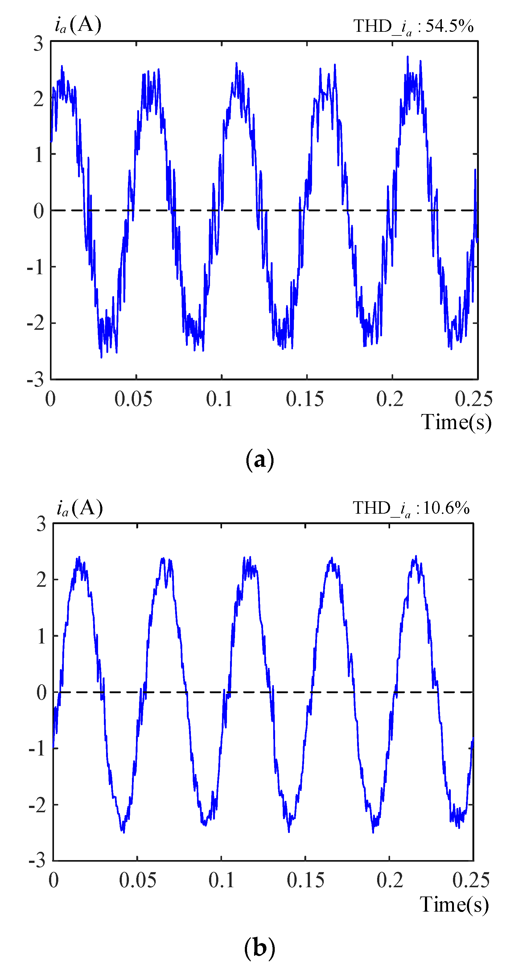
Figure 12a,b show the comparison of the a-phase output current of the hysteresis current control and the proposed extension and compensation SVPWM when the motor is running at 600 rpm under a 1.5 N·m external load. As we can observe, the output current with the proposed method provides lower current harmonics than the hysteresis current control method. The major reason is that hysteresis control uses an infinite gain for a current-loop and then creates high current harmonics. Figure 13a shows the a-phase current and its related sampling signal. The current is detected twice for each switching interval in order to compute the current deviation. Figure 13b shows the extended and compensated SVPWM switching states. In that figure, it can be seen that the sampling interval $T_s$ is 100 μs. The first and second applied voltage vectors are “110” and “010” and are both less than 20 μs. Therefore, these voltage vectors need to be extended at the first stage and then be compensated for at the next stage. Besides that, the switching time for the zero voltage vector reaches 20 μs, and it does not need to be extended. The extended voltage vectors “110” and “010” also need to be compensated for in the opposite direction, which is “001” and “101”, to keep the total time of switching states from changing. Hence, the compensation for switching states “001” and “101” are performed before the end of the switching interval $T_s$. Figure 13c shows the related switching points (broken lines) and sampling points (solid lines). As can be observed, two current sampling points are required for the AVV “110” and “010” and the ZVV “000”.

Figure 14a–d show the $\alpha$ and $\beta$ current responses using the AVV and ZVV algorithms at 60 rpm under a 2 N·m load. Figure 14a shows the $i_{\alpha }$ and $i_{\beta }$ using the AVV and the blue line is $i_{\alpha }$ and the red line is $i_{\beta }$. Figure 14b shows the $i_{\alpha }$ and $i_{\beta }$ using the ZVV and the blue line is $i_{\alpha }$ and the red line is $i_{\beta }$. As we can observe, at low speeds, the ZVV performs better than the AVV with fewer current ripples and current distortions. The reason is that the ZVV uses a lot of zero vectors, but the AVV does not. In addition, the $\alpha \beta$ trajectory for the ZVV is closer to a circle. This is why the ZVV is employed for low-speed ranges. Figure 15a–c illustrate the transitional responses from the ZVV algorithm to the AVV algorithm. Figure 15a shows the estimated and real speeds at about 150 rpm. According to the transition rules in Equations (48)–(50), when the speed is below 60 rpm, the ZVV estimation algorithm is used. However, when the motor is at more than 100 rpm, the AVV rotor estimation algorithm is used. If the speeds are between those two limitations, a weighting factor is considered, which allows the two estimators to transition smoothly to obtain estimated speeds and positions. Figure 15b compares the estimated and real positions, and they are close at a standstill and low-speed ranges. Moreover, during the transitional interval, the estimated and real positions can provide smooth transient responses to demonstrate that the proposed method is practical and useful. Figure 15c demonstrates the estimated position errors. The errors are near six electrical degrees during transitional intervals and then are reduced to two electrical degrees at steady-states. Figure 16a demonstrates the reverse speed responses from 600 rpm to −600 rpm by using a predictive controller. Figure 16b demonstrates the real and estimated position responses, and both of them are similar. The results show that the proposed rotor position estimator can track the real position very well in transient responses and at steady-states. Figure 16c demonstrates the measured estimated rotor position errors, which are near $\pm$4 electrical degrees during the transient responses. The estimated motor position errors in these transient responses are larger than the estimated rotor position errors at a steady-state.

Figure 17a,b show the measured responses of the drive system with different values of external loads. Figure 17a shows the responses when a 1 N·m load is added. As we can observe, the estimated rotor position and estimated rotor speed can follow measured rotor position and rotor speed well. The position error is only $\pm$2 electrical degrees. Figure 17b shows the responses when a 4 N·m load is added, and the estimated position error is near ±3 electrical degrees. Based on these experimental results, the performance of the sensorless drive system can work well at 1 N·m load and 4 N·m load.

Figure 18a demonstrates a comparison of the speed responses by using different controllers. The PI controller has near 10% overshoot, which requires 0.3 s to reach a steady-state. However, the predictive controller only has a 3% overshoot and can reach a steady-state quickly. Figure 18b demonstrates the load disturbance responses at 600 rpm with a 2 N·m load. The PI controller drops by 150 rpm, but the predictive controller drops by only 60 rpm. In addition, the predictive controller has a quicker recovery time than the PI controller. Figure 18c demonstrates the step-input responses at different speeds by using the proposed predictive controller. All of them are linear responses. The reason is that the predictive controller uses more state variables than the PI controller. This demonstrates that the proposed drive system has wide and adjustable ranges, which include different speed ranges.

10. Conclusions

A sensorless DSP-based IPMSM drive system using current deviation detection is implemented in this paper. The ZVV rotor estimating method, which is very suitable for IPMSMs operating at zero-speeds and low-speeds, is originally investigated. Experimental results show that this ZVV estimating method can achieve high-performance sensorless speed control at zero-speed under full load conditions. In addition, a linear combination method, which is the simplest method to combine a ZVV algorithm and an AVV algorithm, is also proposed in this paper. As a result, the IPMSM drive system can be operated from 0 r/min to 3000 r/min. This linear combination method is more easily implemented than fuzzy-logic combination methods.

References

- Piippo, A.; Hinkkanen, M.; Luomi, J. Analysis of an Adaptive Observer for Sensorless Control of Interior Permanent Magnet Synchronous Motors. IEEE Trans. Ind. Electron. 2008, 55, 570–576. [Google Scholar] [CrossRef] [Green Version]
- Sheng, L.; Sheng, L.; Wang, Y.; Fan, M.; Yang, X. Sensorless Control of a Shearer Short-Range Cutting Interior Permanent Magnet Synchronous Motor Based on a New Sliding Mode Observer. IEEE Access 2017, 5, 18439–18450. [Google Scholar] [CrossRef]
- Batzel, T.; Lee, K. Electric Propulsion With the Sensorless Permanent Magnet Synchronous Motor: Model and Approach. IEEE Trans. Energy Convers. 2005, 20, 818–825. [Google Scholar] [CrossRef]
- Zhang, G.; Wang, G.; Xu, D.G.; Zhao, N. ADALINE-Network-Based PLL for Position Sensorless Interior Permanent Magnet Synchronous Motor Drives. IEEE Trans. Power Electron. 2015, 31, 1450–1460. [Google Scholar] [CrossRef]
- Wu, X.; Huang, S.; Liu, K.; Lu, K.; Hu, Y.; Pan, W.; Peng, X. Enhanced Position Sensorless Control Using Bilinear Recursive Least Squares Adaptive Filter for Interior Permanent Magnet Synchronous Motor. IEEE Trans. Power Electron. 2020, 35, 681–698. [Google Scholar] [CrossRef]
- Colli, V.D.; Di Stefano, R.L.; Marignetti, F. A System-on-Chip Sensorless Control for a Permanent-Magnet Synchronous Motor. IEEE Trans. Ind. Electron. 2010, 57, 3822–3829. [Google Scholar] [CrossRef]
- Chen, Z.; Tomita, M.; Doki, S.; Okuma, S. An extended electromotive force model for sensorless control of interior permanent-magnet synchronous motors. IEEE Trans. Ind. Electron. 2003, 50, 288–295. [Google Scholar] [CrossRef]
- Wang, G.; Ding, L.; Li, Z.; Xu, J.; Zhang, G.; Zhan, H.; Ni, R.; Xu, D.G. Enhanced Position Observer Using Second-Order Generalized Integrator for Sensorless Interior Permanent Magnet Synchronous Motor Drives. IEEE Trans. Energy Convers. 2014, 29, 486–495. [Google Scholar] [CrossRef]
- An, Q.-T.; Zhang, J.; An, Q.; Liu, X.; Shamekov, A.; Bi, K. Frequency-Adaptive Complex-Coefficient Filter-Based Enhanced Sliding Mode Observer for Sensorless Control of Permanent Magnet Synchronous Motor Drives. IEEE Trans. Ind. Appl. 2020, 56, 335–343. [Google Scholar] [CrossRef]
- Nguyen, D.; Dutta, R.; Rahman, M.F.; Fletcher, J.E. Performance of a Sensorless Controlled Concentrated-Wound Interior Permanent-Magnet Synchronous Machine at Low and Zero Speed. IEEE Trans. Ind. Electron. 2015, 63, 2016–2026. [Google Scholar] [CrossRef]
- Sun, X.; Cao, J.; Lei, G.; Guo, Y.; Zhu, J. Speed Sensorless Control for Permanent Magnet Synchronous Motors Based on Finite Position Set. IEEE Trans. Ind. Electron. 2020, 67, 6089–6100. [Google Scholar] [CrossRef]
- Barcaro, M.; Morandin, M.; Pradella, T.; Bianchi, N.; Furlan, I. Iron Saturation Impact on High-Frequency Sensorless Control of Synchronous Permanent-Magnet Motor. IEEE Trans. Ind. Appl. 2017, 53, 5470–5478. [Google Scholar] [CrossRef]
- Shinnaka, S. A New Speed-Varying Ellipse Voltage Injection Method for Sensorless Drive of Permanent-Magnet Synchronous Motors With Pole Saliency—New PLL Method Using High-Frequency Current Component Multiplied Signal. IEEE Trans. Ind. Appl. 2008, 44, 777–788. [Google Scholar] [CrossRef]
- Park, N.-C.; Kim, S.-H. Simple sensorless algorithm for interior permanent magnet synchronous motors based on high-frequency voltage injection method. IET Electron. Power Appl. 2014, 8, 68–75. [Google Scholar] [CrossRef]
- Haque, M.; Zhong, L.; Rahman, M. A sensorless initial rotor position estimation scheme for a direct torque controlled interior permanent magnet synchronous motor drive. IEEE Trans. Energy Convers. 2003, 18, 1376–1383. [Google Scholar] [CrossRef]
- Bui, M.X.; Guan, D.; Xiao, D.; Rahman, M.F. A Modified Sensorless Control Scheme for Interior Permanent Magnet Synchronous Motor Over Zero to Rated Speed Range Using Current Derivative Measurements. IEEE Trans. Ind. Electron. 2018, 66, 102–113. [Google Scholar] [CrossRef]
- Wei, M.Y.; Liu, T.H. A high-performance sensorless position control system of a synchronous reluctance motor using dual current-deviation estimating technique. IEEE Trans. Ind. Electron. 2012, 59, 3411–3426. [Google Scholar]
- Raute, R.; Caruana, C.; Staines, C.S.; Cilia, J.; Sumner, M.; Asher, G. Analysis and Compensation of Inverter Nonlinearity Effect on a Sensorless PMSM Drive at Very Low and Zero Speed Operation. IEEE Trans. Ind. Electron. 2010, 57, 4065–4074. [Google Scholar] [CrossRef]
- Hosogaya, Y.; Kubota, H. Position estimating method of IPMSM at low speed region using dq-axis current derivative without high frequency component. In Proceedings of the 2013 IEEE 10th International Conference on Power Electronics and Drive Systems (PEDS), Kitakyushu, Japan, 22–25 April 2013; pp. 1306–1311. [Google Scholar]
- Hua, Y.; Sumner, M.; Asher, G.; Gao, Q.; Saleh, K. Improved sensorless control of a permanent magnet machine using fundamental pulse width modulation excitation. IET Electron. Power Appl. 2011, 5, 359–370. [Google Scholar] [CrossRef] [Green Version]
- Zhang, H.; Liu, W.; Chen, Z.; Mao, S.; Meng, T.; Peng, J.; Jiao, N. A Time-Delay Compensation Method for IPMSM Hybrid Sensorless Drives in Rail Transit Applications. IEEE Trans. Ind. Electron. 2018, 66, 6715–6726. [Google Scholar] [CrossRef]
- Gu, M.; Ogasawara, S.; Takemoto, M. Novel PWM Schemes With Multi SVPWM of Sensorless IPMSM Drives for Reducing Current Ripple. IEEE Trans. Power Electron. 2015, 31, 6461–6475. [Google Scholar] [CrossRef]
- Zhang, Z.; Guo, H.; Liu, Y.; Zhang, Q.; Zhu, P.; Iqbal, R. An Improved Sensorless Control Strategy of Ship IPMSM at Full Speed Range. IEEE Access 2019, 7, 178652–178661. [Google Scholar] [CrossRef]
- Fan, W.; Luo, S.; Zou, J.; Zheng, G. A hybrid speed sensorless control strategy for PMSM based on MRAS and fuzzy control. In Proceedings of the 7th International Power Electronics and Motion Control Conference, Harbin, China, 2–5 June 2012; pp. 2976–2980. [Google Scholar]
- Maciejowski, J.M. Predictive Control with Constraints; Prentice Hall: New York, NY, USA, 2002. [Google Scholar]
- Soeterboek, R. Predictive Control—A Unified Approach; Prentice Hall: New York, NY, USA, 1992. [Google Scholar]
- Camacho, E.F.; Bordons, C. Modern Predictive Control, 2nd ed.; Springer: Berlin/Heidelberg, Germany, 2003. [Google Scholar]
- Wang, L. Model Predictive Control System Design and Implementation Using MATLAB; Springer: Berlin/Heidelberg, Germany, 2009. [Google Scholar]
- Wang, S.; Chai, L.; Yoo, D.; Gan, L.; Ng, K. PID and Predictive Control of Electrical Drives and Power Converters Using MATLAB/Simulink; Wiley: Hoboken, NJ, USA, 2015. [Google Scholar]
- Rodriguez, J.; Cortes, P. Predictive Control of Power Converters and Electrical Drives; Wiley: Hoboken, NJ, USA, 2012. [Google Scholar]
Figure 1.
The coordinate transformation relationship.
Figure 2.
Block diagram of the zero voltage vector (ZVV)-based estimator.
Figure 3.
The main circuit of the mode A+.
Figure 4.
Space-vector pulse width modulation extension and compensation. (a) T1 voltage vector; (b) T2 voltage vector.
Figure 5.
The modulation of inverter and current sampling waveform.
Figure 6.
The linear transfer between ZVV current deviation and active voltage vector (AVV) current deviation.
Figure 7.
Block diagram of the proposed speed-loop predictive controller.
Figure 8.
Implemented system. (a) block diagram; (b) circuit; (c) dynamometer.
Figure 9.
Measured q-axis current deviations to estimated position errors.
Figure 10.
Measured 5 rpm responses. (a) estimated and real positions; (b) estimated and real speeds; (c) estimated position errors.
Figure 11.
Measured waveforms at 0 rpm and 11 N-m load. (a) speeds; (b) positions; (c) estimated position errors.
Figure 12.
Measured phase current at 600 rpm and 1.5 N-m external load. (a) hysteresis current control; (b) proposed SVPWM.
Figure 13.
Measured waveforms. (a) a-phase current and its sampling points; (b) SVPWM; (c) sampling and switching points.
Figure 14.
Measured current waveforms at 60 rpm and 2 N-m load. (a) axis current using AVV; (b) axis current using ZVV; (c) axis trajectory using AVV; (d) axis trajectory using ZVV.
Figure 15.
Measured responses during transition intervals. (a) speeds; (b) positions; (c) position estimated errors.
Figure 16.
Measured responses from 0 rpm to 600 rpm to −600 rpm. (a) speeds; (b) positions; (c) position estimated errors.
Figure 17.
Measured responses of different loads at 600 rpm. (a) 1 N·m; (b) 4 N·m.
Figure 18.
Measured responses at different speeds. (a) 600 rpm transient responses; (b) 600 rpm 2 N·m load responses; (c) different speed responses.
© 2020 by the authors. Licensee MDPI, Basel, Switzerland. This article is an open access article distributed under the terms and conditions of the Creative Commons Attribution (CC BY) license (http://creativecommons.org/licenses/by/4.0/).
Share and Cite
MDPI and ACS Style
Mubarok, M.S.; Liu, T.-H.; Tsai, C.-Y.; Wei, Z.-Y. A Wide-Adjustable Sensorless IPMSM Speed Drive Based on Current Deviation Detection under Space-Vector Modulation. Energies 2020, 13, 4431. https://doi.org/10.3390/en13174431
AMA Style
Mubarok MS, Liu T-H, Tsai C-Y, Wei Z-Y. A Wide-Adjustable Sensorless IPMSM Speed Drive Based on Current Deviation Detection under Space-Vector Modulation. Energies. 2020; 13(17):4431. https://doi.org/10.3390/en13174431
Chicago/Turabian StyleMubarok, Muhammad Syahril, Tian-Hua Liu, Chung-Yuan Tsai, and Zuo-Ying Wei. 2020. "A Wide-Adjustable Sensorless IPMSM Speed Drive Based on Current Deviation Detection under Space-Vector Modulation" Energies 13, no. 17: 4431. https://doi.org/10.3390/en13174431
Note that from the first issue of 2016, this journal uses article numbers instead of page numbers. See further details here.