Comparative Analysis of Summer Upwelling and Downwelling Events in NW Spain: A Model-Observations Approach

Abstract

Upwelling and downwelling processes play a critical role in the connectivity between offshore waters and coastal ecosystems, having relevant implications in terms of intense biogeochemical activity and global fisheries production. A variety of in situ and remote-sensing networks were used in concert with the Iberia–Biscay–Ireland (IBI) circulation forecast system, in order to investigate two persistent upwelling and downwelling events that occurred in the Northwestern (NW) Iberian coastal system during summer 2014. Special emphasis was placed on quality-controlled surface currents provided by a high-frequency radar (HFR), since this land-based technology can effectively monitor the upper layer flow over broad coastal areas in near-real time. The low-frequency spatiotemporal response of the ocean was explored in terms of wind-induced currents’ structures and immediacy of reaction. Mean kinetic energy, divergence and vorticity maps were also calculated for upwelling and downwelling favorable events, in order to verify HFR and IBI capabilities, to accurately resolve the prevailing surface circulation features, such as the locus of a persistent upwelling maximum in the vicinity of Cape Finisterre. This integrated approach proved to be well-founded to efficiently portray the three-dimensional characteristics of the NW Iberian coastal upwelling system regardless of few shortcomings detected in IBI performance, such as the misrepresentation of the most energetic surface dynamics or the overestimation of the cooling and warming associated with upwelling and downwelling conditions, respectively. Finally, the variability of the NW Iberian upwelling system was characterized by means of the development of a novel ocean-based coastal upwelling index (UI), constructed from HFR-derived hourly surface current observations (UI_HFR). The proposed UI_HFR was validated against two traditional UIs for 2014, to assess its credibility. Results suggest that UI_HFR was able to adequately categorize and characterize a wealth of summer upwelling and downwelling events of diverse length and strength, paving the way for future investigations of the subsequent biophysical implications.

1. Introduction

Upwelling (UPW) and downwelling (DOW) phenomena represent a key role in the strong physical connectivity between offshore waters and coastal ecosystems. Wind-driven coastal UPW has been extensively studied along the eastern edges of the world’s major ocean basins, as it has relevant implications on biogeochemical activity and global fisheries production [1,2]. Along-shore equatorward winds modulate an offshore Ekman transport of surface waters that is compensated by the uplift of oxygen-depleted deep cold waters, injecting nutrients into the near-surface euphotic zone and fostering high marine productivity. UPW episodes commonly last 3–10 days [3,4] and can alternate with weak-wind periods (relaxation) or even DOW-favorable events where poleward winds induce a net onshore displacement and subduction of surface coastal waters, allowing larvae communities to reach suitable locations and recruit to the shoreline.

Notwithstanding, extremely active and persistent UPW and DOW events can also impact negatively on coastal ecosystems. During periods of increased offshore advection, some fish and invertebrate populations are exported from coastal habitats and exhibit reduced recruitment success [5]. Equally, an excessive enrichment of surface waters inshore might support the proliferation of harmful algal blooms [6]. The opposite-phase circulation patterns during DOW-favorable wind conditions may be related to the transport and retention of pollutants onto the shoreline, with subsequent biological and socioeconomic consequences.

The Galician UPW system (Northwestern (NW) Iberian Peninsula) extends from 42° N to 44° N (Figure 1). In this region, the seasonality of the ocean dynamics is governed by the relative strengths and latitudinal shifts of the Azores high-pressure and the Iceland low-pressure systems, defining two largely wind-driven oceanographic seasons. The UPW is predominantly a spring–summer phenomenon that is dominated by northerly winds and a prevailing south-westward surface flow. Nevertheless, some out of the season UPW episodes have also been reported in autumn or winter [7]. During the rest of the year, southerly winds prevail which favor DOW events and the subsequent circulation of a narrow surface poleward flow along the NW Iberian shelf edge, the so-called Iberian Poleward Current (IPC) [8].

The UPW intensity in this region has been shown to be strongly dependent on the wind pattern and spatially non-uniform, increasing from the north to the south along the coast [9]. The complexity of the wind field in Galicia is partially associated with the jagged shoreline where Cape Finisterre (CF, denoted in Figure 1b) marks an abrupt change between the zonal north and the meridional west coasts of Galicia. Capes and coastal promontories can modulate UPW processes by inducing important wind stress variations and zones of retention [6]. In this context, CF has been documented to act frequently as the locus of a persistent and localized UPW maximum and recurrent UPW filaments [10]. UPW to the north of CF is also present but generally discontinuous in time, remaining distant from the coast and near the edge of the continental shelf [11]. By contrast, south of CF, UPW episodes are more frequent, intense and generally closer to the coast [12].

The Galician coastal UPW system, albeit profusely investigated, has been mostly described in terms of recurrent patterns and the related spatiotemporal variability of diverse met-ocean parameters (e.g., wind, sea surface temperature, salinity, chlorophyll or silicate, among others) by using data from in situ observational networks, satellite missions or modelling tools [10,11,12,13,14,15]. Growing consideration has been recently given to the landward extension of coastal UPW into the NW Iberian semi-enclosed bays [16,17,18,19].

However, in the present work, notable emphasis is placed on the sea surface current estimations provided by a high-frequency radar (HFR) installed on the Galician shoreline [20,21,22]. Previous initiatives have successfully addressed the characterization of UPW, relaxation and DOW events in other regions, worldwide, by using this consolidated land-based technology, since it is able to effectively monitor the upper layer flow over broad coastal areas in near-real time. The onset, intensity, duration and variability of such coastal phenomena, along with the associated wind-induced circulation and the ecological response, can be featured thanks to the high spatial resolution of HFR-derived surface current maps [23,24,25,26,27,28,29]. Additionally, this cutting-edge technology presents a wide range of practical applications, encompassing search-and-rescue emergencies, accidental spillages of pollutants, harbor management or the skill assessment of ocean numerical models [30,31].

Given the positive synergies between observations and numerical models at coastal scales [32,33], the main objective of this paper is twofold. Firstly, to showcase the ability of the Iberia–Biscay–Ireland (IBI) ocean forecast system [34] (Figure 1a) to adequately reproduce the three-dimensional features of two persistent UPW and DOW events during summer 2014 in the NW Iberian Peninsula (Figure 1b). To the extent that UPW and DOW circulation patterns have been previously reported to be recurring [7], their presence also becomes predictable, and thus anticipatory strategies can be efficiently prompted to face environmental affairs such as larval transport pathways or the destination of accidental oil spills [29]. To this end, quality-controlled HFR hourly current estimations, satellite products and in situ observations from buoys and a Conductivity–Temperature–Depth (CTD) device were used in concert with IBI hydrodynamic model. A thorough characterization of the ocean signatures associated with UPW and DOW activities can be achieved thanks to their complementary and interdependent nature. While traditional instrumented platforms provide a close approximation of “ground truth” for remotely sensed estimations, HFR observations enhance numerical simulations by resolving fine-scale processes in intricate regions with complex-geometry configurations. In turn, hydrodynamic models can reciprocally serve as integrative connectors of sparse in situ observations and gappy HFR surface current maps by offering a seamless predictive picture of the three-dimensional ocean state. Secondly and most importantly, to characterize the variability of the NW Iberian UPW system through the development of a novel basic ocean-based coastal UPW index, generated from HFR-derived hourly surface current estimations (UI_HFR). Assuming the immediate oceanic response to wind forcing, the proposed high-frequency index can act as a proxy of UPW and DOW conditions. In this context, UI_HFR was compared with two preexisting six-hourly UPW indexes for the entire 2014, with the purpose of evaluating its consistency and variability. Likewise, the ability of UI_HFR to categorize UPW and DOW events during summer 2014 was also qualitatively assessed.

This work is structured as follows: Section 2 outlines the observational and modelled data sources, along with the methodology adopted. Results are presented and interpreted in Section 3. A comprehensive discussion and future work are addressed in Section 4. Finally, principal conclusions are drawn in Section 5.

2. Materials and Methods

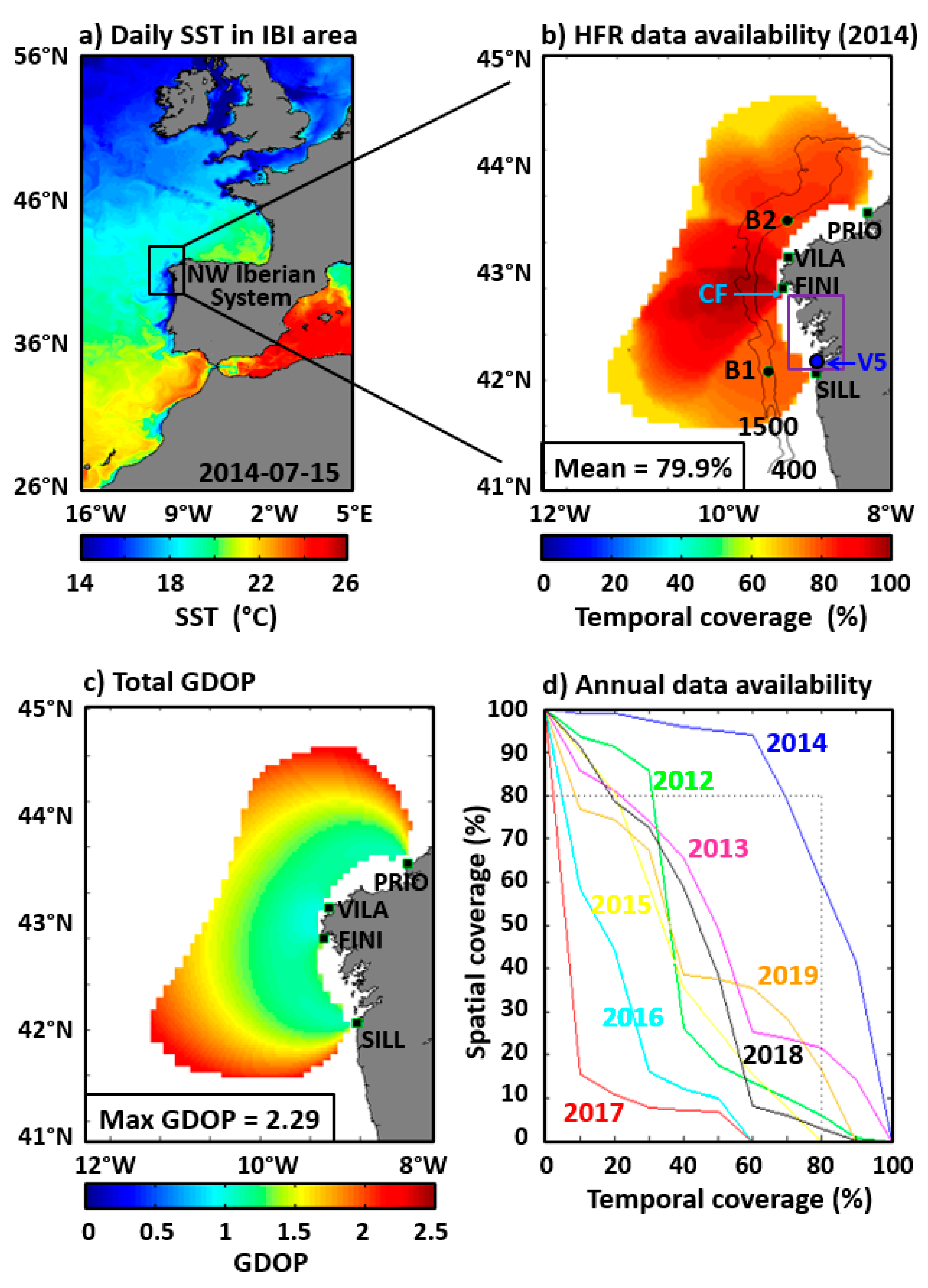
2.1. The Galician HFR System

A four-site long-range CODAR SeaSonde network, deployed along the Galician Coast (Figure 1b), was used in this work. The first two sites (owned by Puertos del Estado) were deployed in 2004: Silleiro (SILL) and Finisterre (FINI). Afterward, the network was extended northward, in December 2011, by installing two additional sites on phased approach: Vilán (VILA) and Prior (PRIO), owned by INTECMAR–Xunta de Galicia. Each single radar site operates at a central frequency of 4.86 MHz, with a 29.41 KHz bandwidth, measuring the following:

(i)

Hourly radial currents, moving toward or away from the site, that are representative of the upper 2 m of the water column. The maximum current speed, horizontal range and angular resolution are 100 cm·s⁻¹, 200 km and 5°, respectively. All of those radial current vectors (from two or several sites) within a predefined search radius of 25 km are geometrically combined by applying an unweighted least squares fitting algorithm [35] to estimate hourly total current vectors on a Cartesian regular mesh of 6 × 6 km horizontal resolution.

(ii)

Thirty-minute wave estimations for five range cells, regularly spaced every 5.1 km, which extend radially from the site. For further details about this dataset, the reader is referred to Reference [22], as the present work is mainly focused on surface circulation.

The hourly data availability during 2014 was significantly high in the center of the domain (above 90%), decreasing to 60–70% in the westernmost borders (Figure 1b). The spatially averaged data availability was almost 80% for the entire year, revealing that the HFR system performed within acceptable ranges despite the severe FINI breakdown since November 2014.

The specific geometry of the HFR domain and, hence, the intersection angles of radial vectors handicap the accuracy of the total current vectors resolved at each grid point. Such a source of uncertainty is quantified by a dimensionless parameter denominated Geometrical Dilution of Precision (GDOP) [36], which typically increases with the distance from the HFR sites. In this work, a cutoff filter of 2.3 was imposed for the GDOP, to get rid of those estimations affected by higher uncertainties. Consequently, GDOP values remain below 2 in the core of the spatial domain, reaching maximum values of 2.29 at the boundaries of the HFR areal coverage (Figure 1c).

Although this four-site HFR system has been working operationally since 2012, the continued data provision was dramatically impacted by a number of serious breakdowns, mainly due to severe weather episodes that typically battered the Galician Coast during wintertime. Additionally, the global economic recession also challenged the financial support to preserve the infrastructure core already implemented. Since the dataset corresponding to 2014 presented both the highest temporal availability and maximum areal coverage (Figure 1d), this work was focused on UPW and DOW events occurred during this specific year.

Finally, note that the present system is part of the cross-border HFR network in the NW of the Iberian Peninsula, reinforced in the framework of the RADAR ON RAIA project (Interreg V, a Spain–Portugal cooperative program). This initiative aims at capitalizing oceanographic knowledge through the extension and consolidation of this HFR network and the development of user-oriented products.

2.2. In Situ Buoys

Basic features of two deep ocean buoys, deployed within the HFR footprint (Figure 1b), are gathered in

Table 1. Description of the buoys deployed within HFR coverage.

Buoy	Name	Model	Deployment	Longitude	Latitude	Depth	Sampling
B1	Silleiro	Seawatch	1998	9.44°W	42.12°N	600 m	1 h
B2	Vilano	Seawatch	1998	9.22°W	43.50°N	386 m	1 h

. Both in situ devices collect quality-controlled estimations of sea surface temperature (SST), among other physical parameters. Furthermore, since B1 buoy is equipped with an acoustic current meter and a wind sensor, it also provides hourly averaged current and wind vectors at 3.5 m depth and 3 m height, respectively.

2.3. Upwelling Indexes

Annual (2014) time series of two coastal upwelling indexes (UIs), based on 6-hourly data of sea level pressure (UI_BAIXAS) and wind (UI_B1), were used as benchmark in this work to assess the credibility of the proposed ocean-based index. Both are freely available at the IEO (Instituto Español de Oceanografía) website: http://www.indicedeafloramiento.ieo.es/index_en.html. UI_BAIXAS, which was calculated at 42°N, 10°W, was derived from the FNMOC (Fleet Numerical Meteorology and Oceanography Center, US Navy) database. UI_B1 was computed by using wind data obtained from B1 buoy. For further information about these two UIs, the reader is referred to Reference [15].

2.4. CTD Device

Water temperature and salinity profiles were measured on a weekly basis, at the inner part of the Rías Baixas, using a CTD device (denoted by a purple box and a blue dot, respectively, in Figure 1b), which belongs to a network of 43 oceanographic stations operated by INTECMAR. Since the IBI ocean forecast system is not able to adequately resolve the jagged intricate coastline deep inside the Rías Baixas, only one of the outermost CTD stations was selected to conduct the comparisons: V5 (located at 42.18°N–8.87°W).

2.5. Satellite-Derived Products

Two daily satellite-derived products, gap-filled and interpolated on a regular grid, were used in this study, to characterize the UPW and DOW episodes: the first one for the SST (OSTIA: Operational Sea Surface Temperature and Ice Analysis) and the second one for the chlorophyll (CHL) concentration. Essential features of both products are summarized in

Table 2. Description of the satellite products used in this work.

Name	Variable	Type	Level	Resolution	Frequency	Provider
OSTIA	SST	L4 (gap-filled)	Surface	0.05°	Daily	UK MetOffice
CHLL4	CHL	L4 (gap-filled)	Surface	0.01°	Daily	Ocean Color TAC

OSTIA = Operational Sea Surface Temperature and Ice Analysis. CHL = chlorophyll. TAC = Thematic Assembly Center.

. Additional information can be obtained in their respective Product User Manuals (PUMs), freely accessible through the Copernicus Marine Environment Monitoring Service (CMEMS) catalogue (https://marine.copernicus.eu/)

2.6. IBI Ocean Forecast System

The CMEMS IBI operational suite consists of a NEMO model v3.6 [37] application, run daily over a regional grid (Figure 1a) with a horizontal resolution of $~$3 km and 50 unevenly distributed vertical levels. A best estimate of the ocean state (also called “hindcast”) and a five-day-ahead forecast are routinely produced for a number of hydrodynamic variables: temperature, salinity, mixed layer depth, zonal and meridional velocity currents and sea surface height, among others. While hourly averaged estimations are provided at the sea surface, daily averaged values are computed for the rest of the three-dimensional water column. The system is driven every 3 h by high-resolution (1/8°) meteorological forcings provided by the European Center for Medium-Range Weather Forecast (ECMWF). Initial and lateral open-boundary conditions, imposed from daily 3D outputs from the parent system (CMEMS GLOBAL), are complemented with 11 tidal harmonics. The freshwater discharges are prescribed through 33 points corresponding to the main rivers present in the IBI area. This version of IBI ocean forecast system does not include an assimilation scheme. For further technical specifications, the reader is referred to Reference [38].

2.7. Methods

A battery of basic processing steps was applied to the sea surface temperature, salinity, current velocity and wind observations. Given the focus on the low-frequency characteristics of the flow field, any short gap of 6 h or less was filled by applying linear interpolation.

The agreement between two datasets was evaluated by computing a variety of conventional statistics: mean ($\overline{\mathrm{x}}$) and the related standard deviation (σ), mean absolute difference (MAD), root mean squared error (RMSE), scalar correlation, complex correlation (CC) coefficient $(\rho$) and the associated phase ($\mathsf{\theta },\mathrm{in}\mathrm{degrees}$) between two vector fields [39], defined as ${\mathrm{w}}_1\left(\mathrm{t}\right)={\mathrm{u}}_1\left(\mathrm{t}\right)+{\mathrm{iv}}_1\left(\mathrm{t}\right)$ and ${\mathrm{w}}_2\left(\mathrm{t}\right)={\mathrm{u}}_2\left(\mathrm{t}\right)+{\mathrm{iv}}_2\left(\mathrm{t}\right)$, among others.

$$\overline{\mathrm{x}}=\frac{1}{\mathrm{N}}{\displaystyle \sum }_{\mathrm{i}=1}^{\mathrm{N}}{\mathrm{x}}_{\mathrm{i}}$$

(1)

$$\mathsf{\sigma }=\sqrt{\frac{1}{\mathrm{N}-1}{\displaystyle \sum }_{\mathrm{i}=1}^{\mathrm{N}}{\left({\mathrm{x}}_{\mathrm{i}}-\overline{\mathrm{x}}\right)}^2}$$

(2)

$$\mathrm{MAD}=\frac{1}{\mathrm{N}}{{\displaystyle \sum }}_{\mathrm{i}=1}^{\mathrm{N}}\left|{\mathrm{x}}_{\mathrm{i}}-{\mathrm{y}}_{\mathrm{i}}\right|$$

(3)

$$\mathrm{RMSE}=\sqrt{\frac{1}{\mathrm{N}}{\displaystyle \sum }_{\mathrm{i}=1}^{\mathrm{N}}{\left({\mathrm{x}}_{\mathrm{i}}-{\mathrm{y}}_{\mathrm{i}}\right)}^2}$$

(4)

$$\mathrm{Correlation}=\frac{1}{\mathrm{N}-1}{\displaystyle \sum }_{\mathrm{i}=1}^{\mathrm{N}}\left(\frac{{\mathrm{x}}_{\mathrm{i}}-\overline{\mathrm{x}}}{{\mathsf{\sigma }}_{\mathrm{x}}}\right)\left(\frac{{\mathrm{y}}_{\mathrm{i}}-\overline{\mathrm{y}}}{{\mathsf{\sigma }}_{\mathrm{y}}}\right)$$

(5)

$$\rho =\frac{\langle {\mathrm{u}}_1{\mathrm{u}}_2+{\mathrm{v}}_1{\mathrm{v}}_2\rangle }{\sqrt{\langle {\mathrm{u}}_1^2+{\mathrm{v}}_1^2\rangle }\sqrt{\langle {\mathrm{u}}_1+{\mathrm{v}}_1\rangle }}+\mathrm{i}\frac{\langle {\mathrm{u}}_1{\mathrm{u}}_2-{\mathrm{v}}_1{\mathrm{v}}_2\rangle }{\sqrt{\langle {\mathrm{u}}_1^2+{\mathrm{v}}_1^2\rangle }\sqrt{\langle {\mathrm{u}}_1+{\mathrm{v}}_1\rangle }}$$

(6)

$$\mathsf{\theta }=ta{n}^{-1}\frac{\langle {\mathrm{u}}_1{\mathrm{v}}_2-{\mathrm{u}}_2{\mathrm{v}}_1\rangle }{\langle {\mathrm{u}}_1{\mathrm{u}}_2-{\mathrm{v}}_1{\mathrm{v}}_2\rangle }$$

(7)

HFR estimations were bilinearly interpolated on the finer resolution IBI hindcast mesh, in order to adequately compare both datasets in a common regular domain. The prevailing wind-driven surface circulation during UPW and DOW episodes was examined from a Eulerian perspective, by means of 10-day averaged patterns of surface currents. Complementarily, spatial maps of the CC between observed and modelled current velocity vectors were also calculated, to study their concordance and infer those areas where the model performance might be more consistent. With the purpose of better understanding the flow dynamics, we estimated a wealth of ancillary diagnostics, such as the horizontal divergence (DIV), the vorticity (VOR) and the mean kinetic energy (MKE).

$$\mathrm{DIV}=\frac{\partial \mathrm{u}}{\partial \mathrm{x}}+ \frac{\partial \mathrm{v}}{\partial \mathrm{y}}$$

(8)

$$\mathrm{VOR}=\frac{\partial \mathrm{v}}{\partial \mathrm{x}}- \frac{\partial \mathrm{u}}{\partial \mathrm{y}}$$

(9)

$$\mathrm{MKE}=\frac{1}{\mathrm{N}}{\displaystyle \sum }_{\mathrm{i}=1}^{\mathrm{N}}\frac{1}{2}\left({\mathrm{u}}_{\mathrm{i}}^2+{\mathrm{v}}_{\mathrm{i}}^2\right)$$

(10)

where N, u and v represent the total number of data, the zonal and meridional velocity fields, respectively.

Another method to investigate the flow dynamics and seawater dispersion is the Instantaneous Rate of Separation (IROS), which is a Eulerian metric that determines how an infinitesimally small particle will be moved by an instantaneous velocity field, and is equal to the finite-time Lyapunov exponent (FTLE) at time t = 0 [40]. This diagnostic, successfully used in previous studies with HFR data [41,42], can be calculated from the sum of divergence and total strain:

$$\mathrm{IROS}=\left(\frac{\partial \mathrm{u}}{\partial \mathrm{x}}+\frac{\partial \mathrm{v}}{\partial \mathrm{y}}\right)+\sqrt{{\left(\frac{\partial \mathrm{v}}{\partial \mathrm{x}}+\frac{\partial \mathrm{u}}{\partial \mathrm{y}}\right)}^2+{\left(\frac{\partial \mathrm{u}}{\partial \mathrm{x}}-\frac{\partial \mathrm{v}}{\partial \mathrm{y}}\right)}^2}$$

(11)

While the FTLE unveils a variety of features that dominate over longer time periods, IROS indicates how the particles react in the selected moment, estimating particle separation from a snapshot without integrating the flow over time. Since IROS does not require time integration, it is a rather simple and useful diagnostic to examine mean characteristics of the flow in the NW upwelling system. High values of IROS indicate potential regions of elevated particle dispersion, which has relevant implications for cross-shelf exchange of passive tracers between offshore and coastal waters.

Finally, a novel ocean-based coastal upwelling index (UI_HFR) was developed for the NW Iberian upwelling system. Assuming a direct relationship between atmospheric forcing and the prompt response of the upper ocean layer, a rather simple index was constructed from HFR-derived hourly estimations of sea surface currents, spatially averaged over the Galician continental shelf. Similar to the classical Ekman upwelling index [43], the UI_HFR is defined as follows:

$${\mathrm{UI}}_{\mathrm{HFR}}\left({\mathrm{m}}^3·{\mathrm{s}}^{-1}·{\mathrm{km}}^{-1}\right)=-\frac{{\rho }_A·C_d\sqrt{{\mathrm{u}}^2+{\mathrm{v}}^2}·\mathrm{v}}{f·{\rho }_w}·3\times {10}^6$$

(12)

where ρ_w is the seawater density (1025 kg·m⁻³), C_d is a dimensionless empirical drag coefficient (1.4 × 10⁻³), ρ_A is the air density in normal conditions (1.22 kg·m⁻³) and f is the Coriolis parameter. In this case, u and v denote the detided hourly time series of HFR zonal and meridional current velocities (m·s⁻¹), respectively. The sign is changed to define positive (negative) magnitudes of UI_HFR as response of the predominant equatorward (poleward) surface flow over the Galician shelf.

3. Results

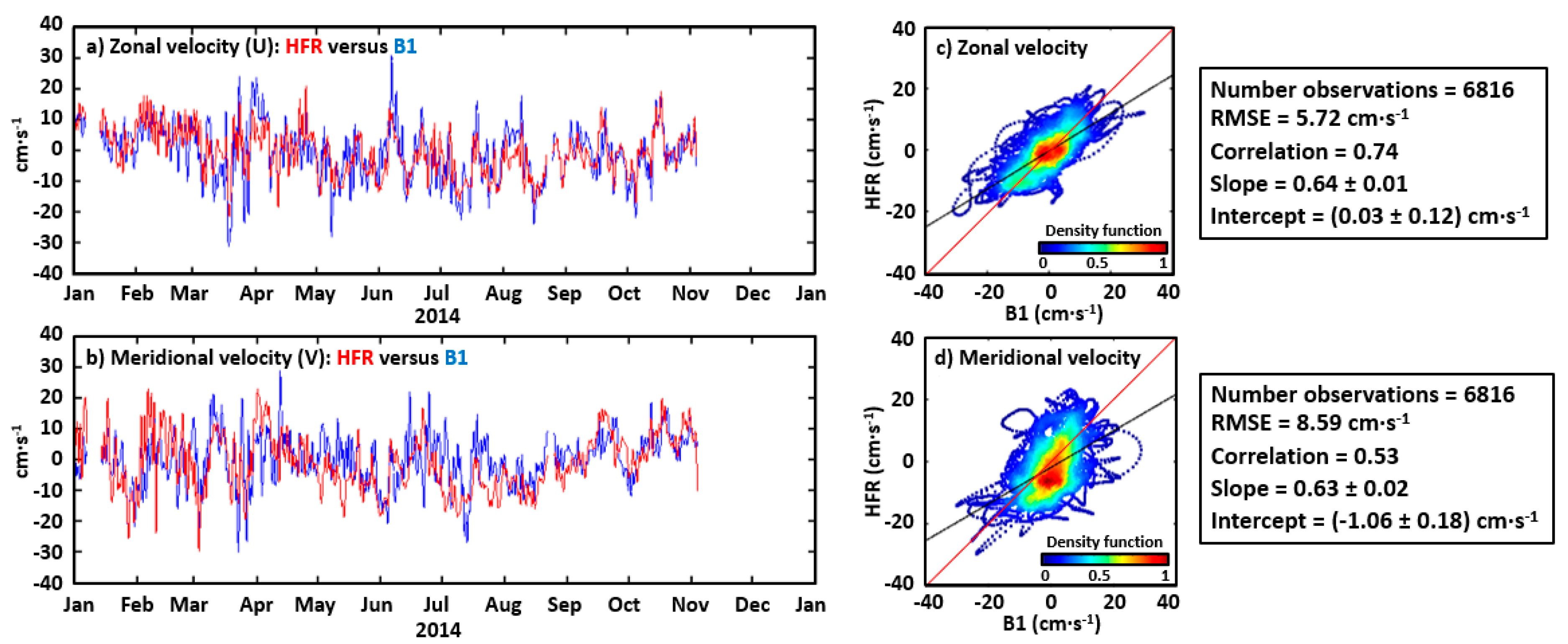
3.1. Skill Assessment of HFR Estimations

The credibility of HFR-derived current data has been extensively assessed worldwide [44,45,46] by conducting quantitative comparisons with independent observations provided by in situ platforms such as drifters, acoustic Doppler current profilers (ADCPs) or current meters (CMs). Routine validation exercises are pertinent since the accuracy of remotely sensed estimations might be negatively affected by inherent problems of radar technology such as radio frequency interferences, reflections from moving ships, antenna pattern distortion, adverse environmental conditions or hardware failures, among others [47].

In this context, a preliminary skill assessment of the Galician HFR system was performed for 2014. Hourly HFR current estimations at the grid point closest to B1 location were compared with concurrent observations from a CM installed in B1 (Figure 1b). Comparisons were attempted for both the zonal and meridional sub-inertial currents, obtained after applying a 10th-order digital low-pass Butterworth filter with a cutoff period of 30 h [48]. This scheme is adequate, as the study is mainly concerned with the low-frequency characteristics of the surface flow.

The visual resemblance between the HFR and CM time series is significantly high for both current components (Figure 2a,b), with correlation coefficient and RMSE values emerging in the ranges (0.53–0.74) and (5.72–8.59) cm·s⁻¹, respectively. These figures are in accordance with similar investigations previously conducted in the Iberian waters (

Table 3. Series of prior studies dealing with the validation of HFR total current vectors against in situ observations in the Iberian waters.

Reference	HFR (MHz)	Region	RMSE/Correlation
[49]	CODAR SeaSonde (4.86)	Galicia	5–7 cm·s−1/0.68–0.88
[50]	CODAR SeaSonde (4.53)	Bay of Biscay	8–13 cm·s−1/0.34–0.86
[51]	CODAR SeaSonde (4.53)	Bay of Biscay	8–15 cm·s−1/0.27–0.67
[52]	CODAR SeaSonde (27)	Strait of Gibraltar	8–22 cm·s−1/0.31–0.81
[53]	CODAR SeaSonde (13.5)	Ibiza Channel	7–12 cm·s−1/0.59–0.72
[20]	CODAR SeaSonde (4.86)	Galicia	8–13 cm·s−1/0.56–0.74

). According to the best linear fit of scatterplots, remote-sensed estimations seem to underestimate, to a small extent, the speed of the surface currents observed at B1 (Figure 2c,d).

3.2. Skill of IBI to Reproduce Two Upwelling/Downwelling Events

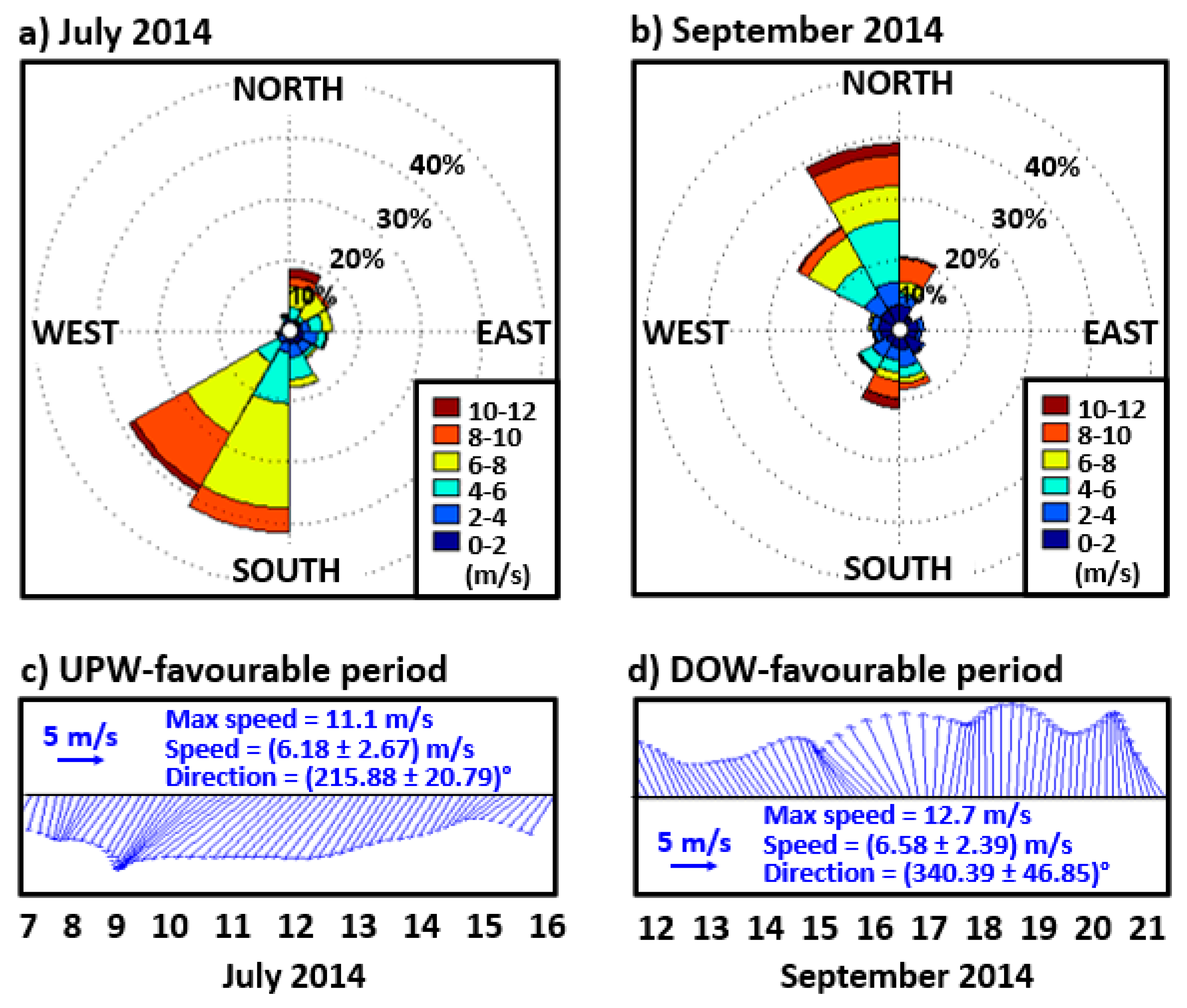
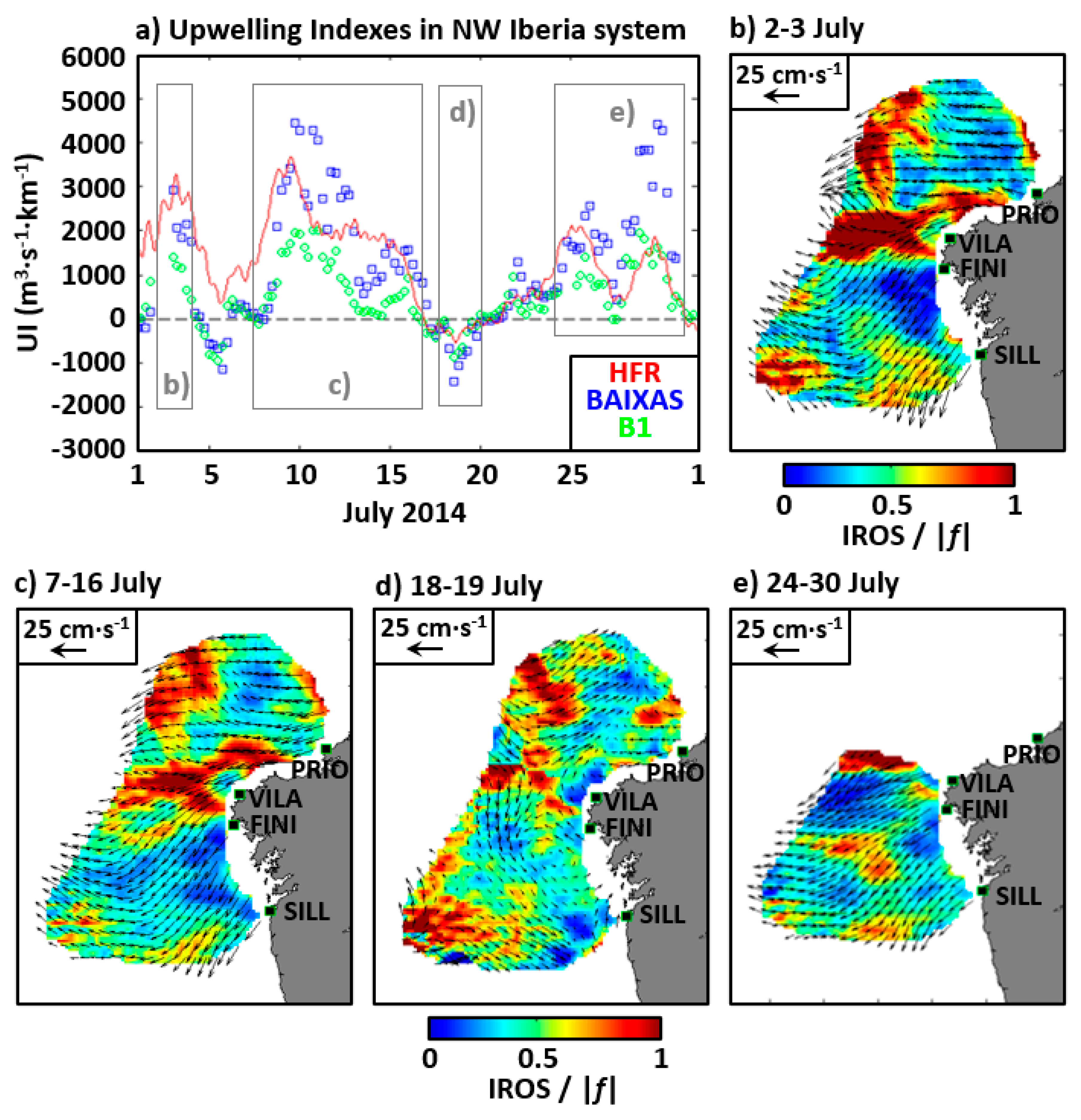
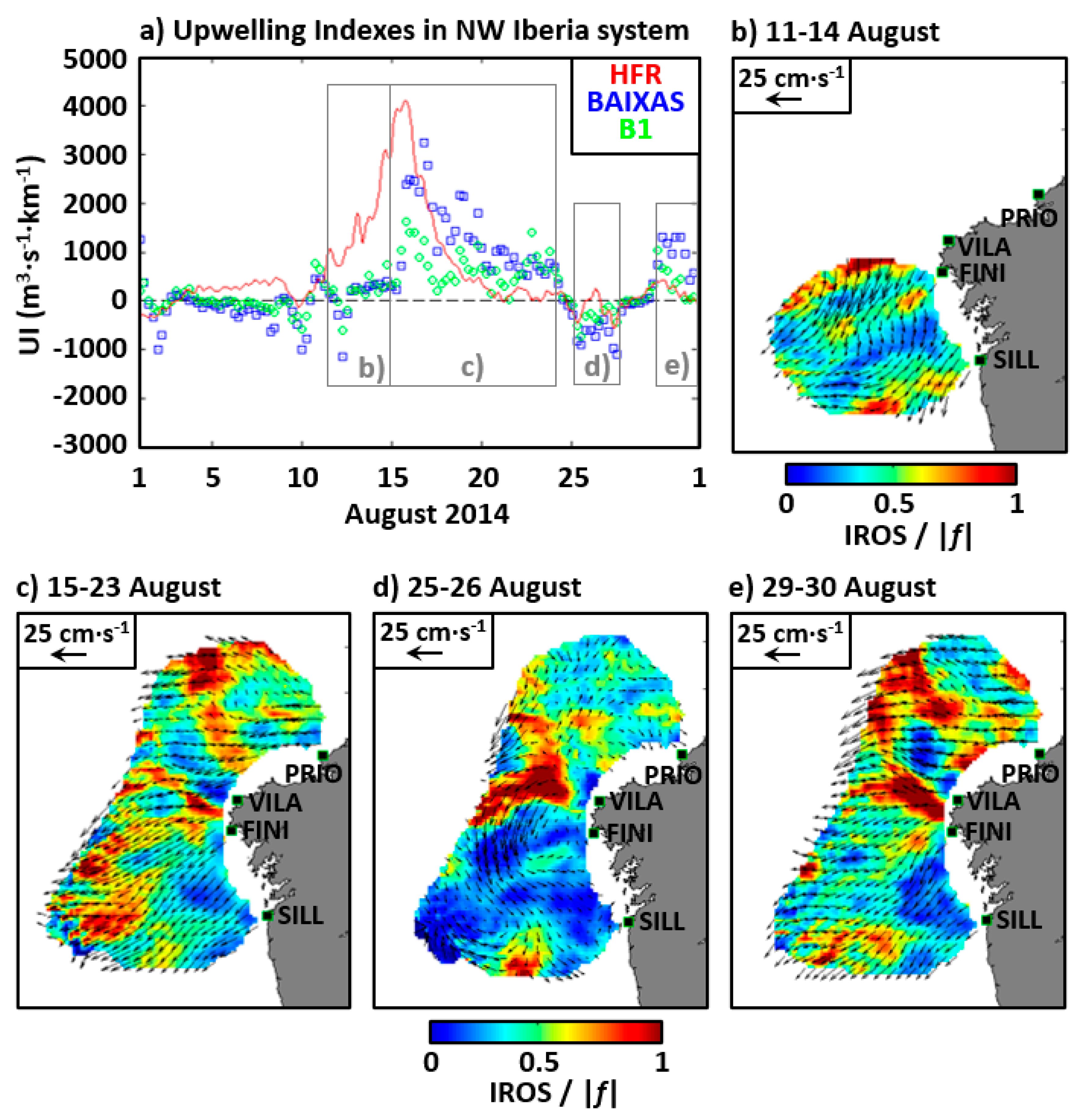
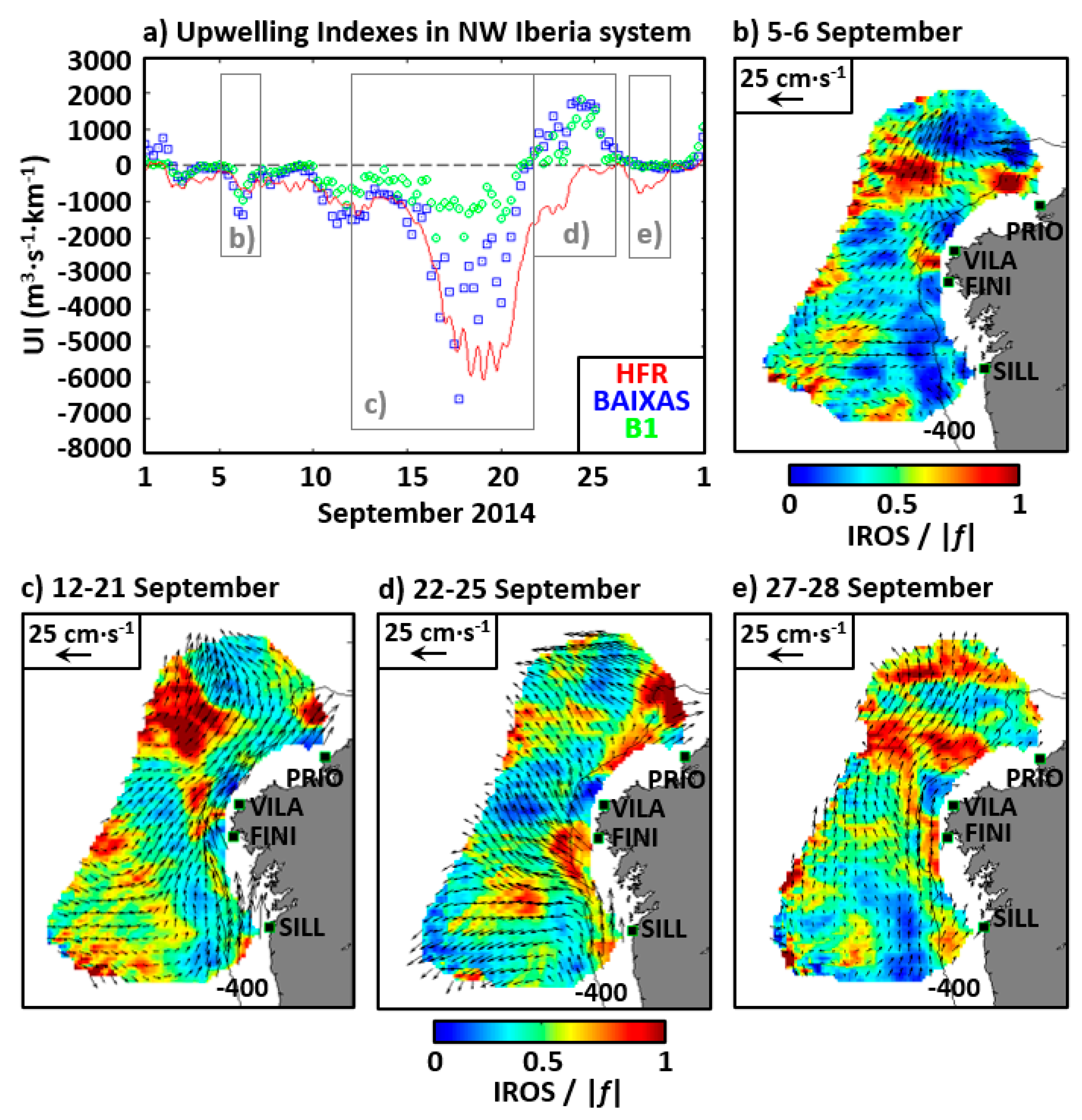
3.2.1. Selection of Upwelling and Downwelling Events

Although observations at a single point are unlikely to be fully representative of the oceanographic conditions found over the entire study area, hourly wind measured at B1 was low-pass filtered, depicted every 3 h and later analyzed as a proxy for the local open sea wind regime. An abrupt shift in local wind directions, from July to September 2014, is evidenced in monthly wind roses (Figure 3). Northerly and northeasterly winds clearly predominated in July (Figure 3a). By contrast, persistent southerly and southeasterly winds prevailed during September 2014, with strong gusts up to 12.7 m·s⁻¹ (Figure 3b). Following References [54,55], we identified two anomalously long-lasting UPW and DOW events during summer 2014, by looking at persistently dominant wind directions and sustained high wind speeds above a predefined threshold of 3 m·s⁻¹. The meridional wind regime was permanently directed southward and northward, respectively, during 10 consecutive days when no relevant relaxation (below the imposed cutoff) in between was exhibited (Figure 3c,d). Although Reference [56] already documented the UPW conditions and the resulting coastal dynamics as response to two unusually persistent 10-day wind episodes, transient UPW conditions tend to last shorter time [3,4], with an average length of ~3 days on the Galician shelf [19].

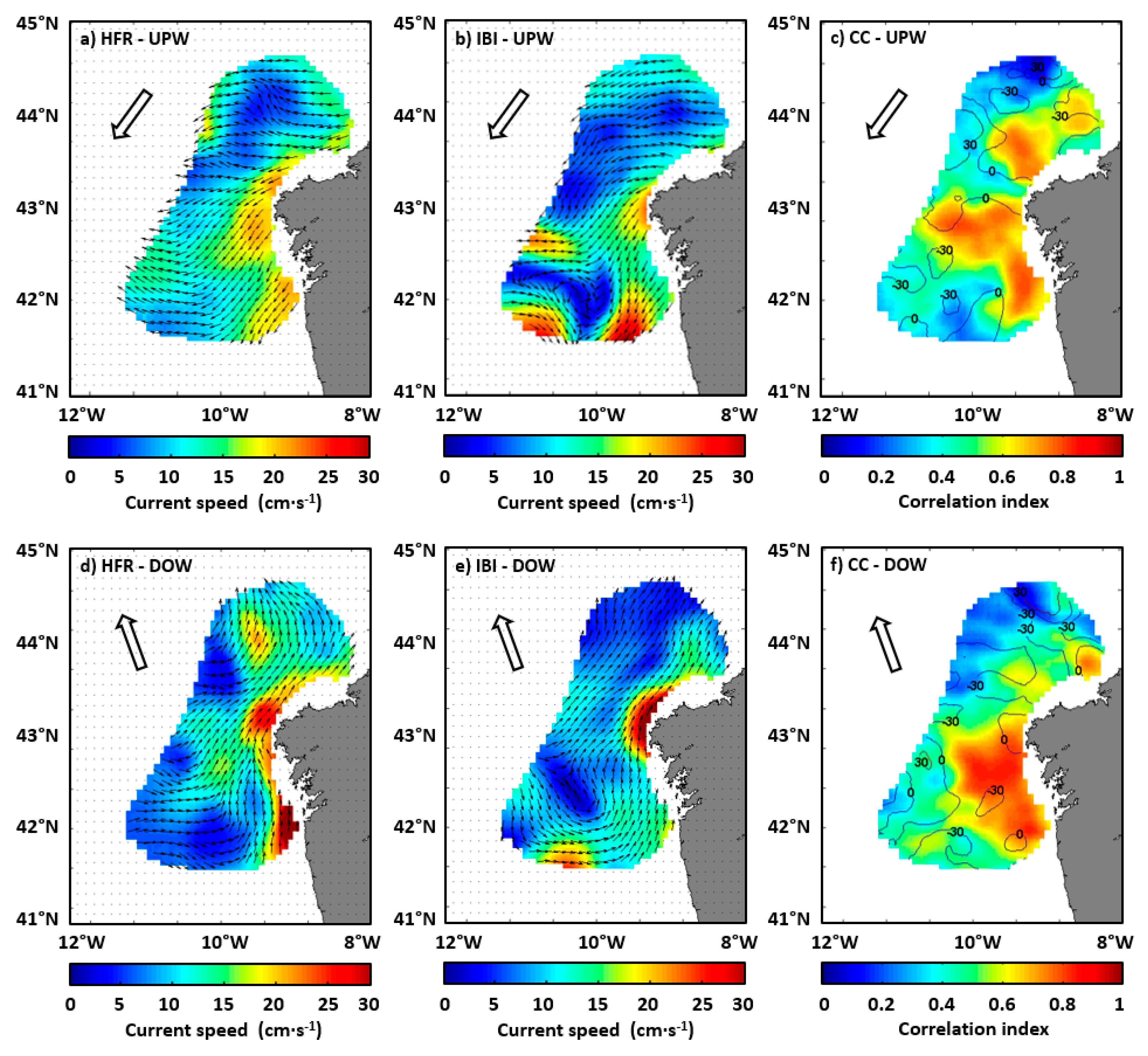
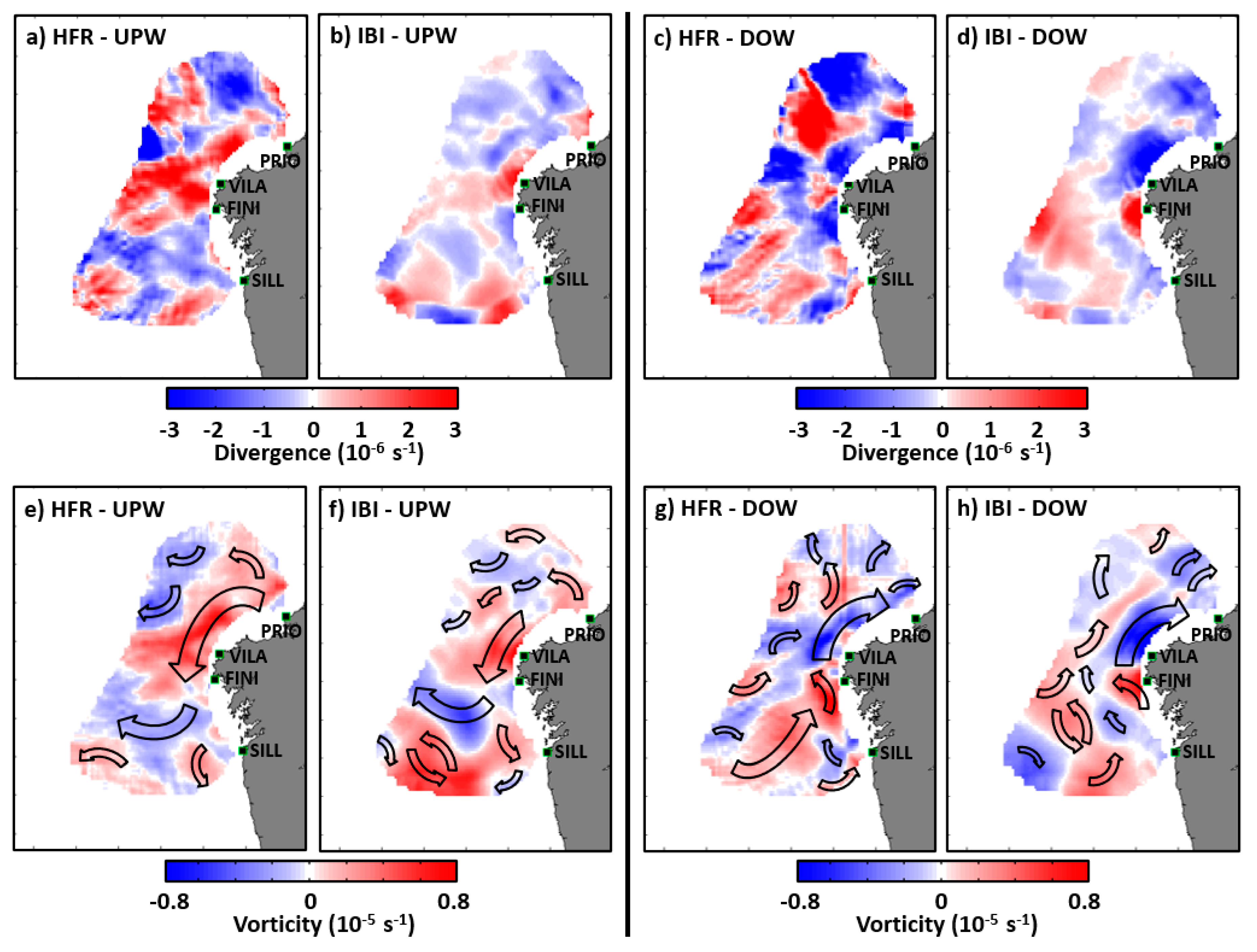
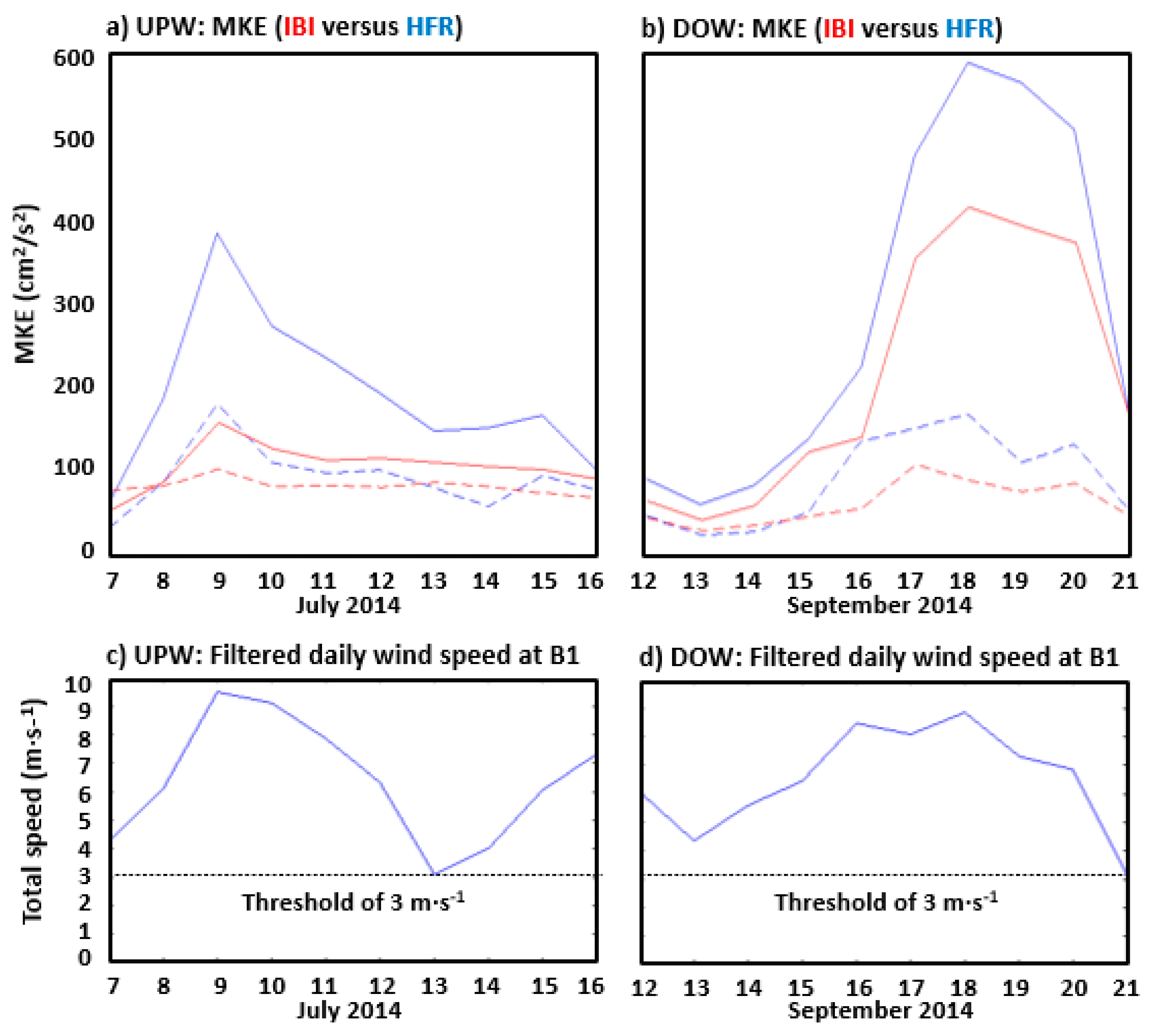
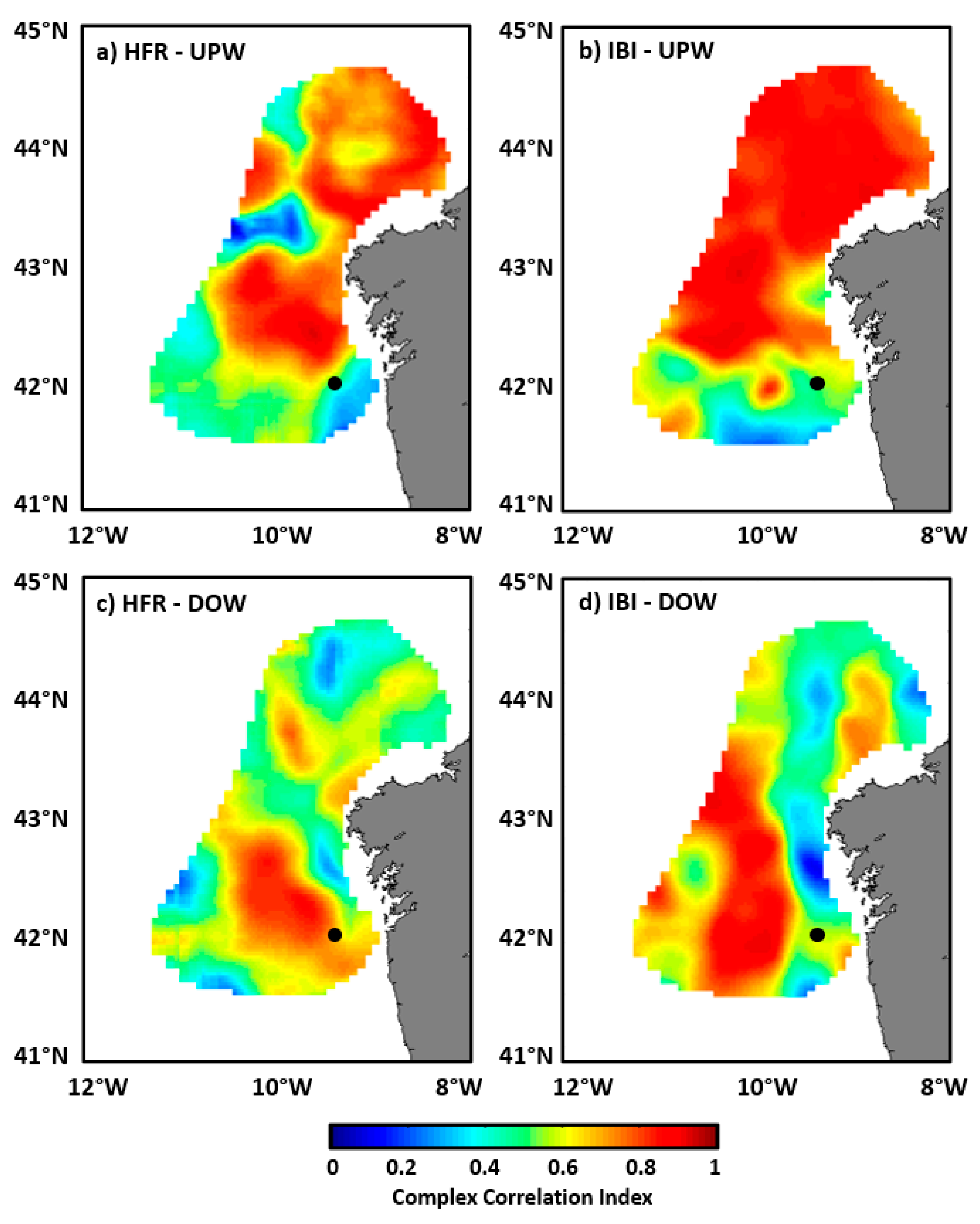
3.2.2. Analysis of the Surface Circulation

According to the significant resemblance between observed and modelled mean circulation patterns, it can be stated that IBI seems to properly resolve the large-scale surface dynamics in the study area for both UPW and DOW events (Figure 4). The UPW episode is characterized by a wind-induced southwestward flow, with an offshore advection of coastal waters to the open ocean, in accordance with Ekman´s theory that postulates a net movement to the right of wind direction in the northern hemisphere (Figure 4a,b). An advective acceleration of surface currents speed over the continental shelf is revealed in both datasets, especially in the periphery of CF.

By contrast, a rather uniform poleward surface circulation is evidenced in response to prevailing southerly winds during the DOW episode (Figure 4d,e). On the southern inner shelf, the interplay between the existing topographic barriers and the cross-shore transport led to a marked directional change of the coastal flow to the left, intensified in form of a narrow jet, the well-documented IPC, which circulated along the NW Iberian shelf edge [8,57]. Since river plumes are mainly confined landward during DOW conditions [58], this northward coastal jet apparently was not significantly perturbated by impulsive-type freshwater outflows at this stage of the year.

The primary IBI-HFR disagreement arises from the presence, detached from the coast, of a southern counter-clockwise eddy-like circulation structure (Figure 4b) and an elongated meander (Figure 4e) in the modelled currents under UPW and DOW conditions, respectively. Conversely, the HFR-derived circulation patterns seem to be more homogeneous, with no proof of the existence of any coherent vortex (Figure 4a,d).

Maps of CC reflect an overall higher IBI–HFR correspondence in regions close to the shoreline, with the CC index and the related phase lying in the ranges (0.6–0.9) and (0–10°), respectively, for both the UPW (Figure 4c) and DOW (Figure 4f) events. These outcomes are in line with earlier works dealing with the same topic [59,60], where the CC coefficients and the associated (absolute) phases were reported to lie between 0.2 and 0.8 and between 0° and 20°, respectively. The degree of accordance tends to decline in areas near the limits of the HFR footprint, where higher GDOP values are indeed encountered, especially within the northernmost sectors (Figure 1c): the CC coefficient drops to (0.2–0.4), and the associated phase increases up to 30° (in absolute value) in nearby edges of the HFR domain (Figure 4c,f). Accordingly, Reference [59] also obtained lower CC coefficients ($~$0.4) in remote areas, distant from the coastline. Spatially averaged skill metrics that were derived from the IBI–HFR comparison of surface currents for the two selected events are gathered in

Table 4. Overview of skill metrics derived from IBI–HFR comparison of surface currents for the selected UPW and DOW events, spatially averaged over the entire common domain (Entire) and exclusively over the Galician continental shelf (Shelf).

Skill Metric	UPW-Entire	UPW-Shelf	DOW-Entire	DOW-Shelf
Zonal RMSE (cm·s−1)	11.00	9.59	11.77	10.48
Meridional RMSE (cm·s−1)	10.94	8.26	12.68	11.87
Zonal correlation	0.51	0.61	0.51	0.63
Meridional correlation	0.44	0.58	0.42	0.61
CC	0.50	0.63	0.50	0.66

. IBI performance was similar for both episodes, with comparable levels of accuracy for the zonal and meridional current components. Better statistics were obtained over the continental shelf than in open waters.

Horizontal divergence at the sea surface was calculated to discriminate zones of contraction and expansion of the flow where vertical flux might be significant in terms of proximal origins and destinations of water particles [27]. Positive surface divergence is generally associated with a convergence at deeper levels and the subsequent vertical uplift of waters (i.e., UPW). By contrast, regions of negative surface divergence (i.e., convergence) are related to downward motions to lower levels (i.e., DOW). Therefore, in order to unveil localized areas of UPW and DOW conditions, maps of horizontal divergence were computed by using both the HFR and IBI datasets (Figure 5). Under UPW-favorable winds, a common peak of positive divergence is exposed in the central portion of the domain (43° N of latitude) and also in the periphery of CF, indicating accumulated upward vertical motions and strong UPW. A large belt of positive coastal divergence, extended from FINI to PRIO radar sites, is exhibited in the HFR dataset (Figure 5a). On the contrary, in the case of IBI, the divergence over the continental shelf seems to be weaker and alternated with areas of horizontal convergence (Figure 5b). Under dominant southerly winds, strong coastal convergence is evidenced north of CF, indicating that the surface flow is presumably sinking downward (Figure 5c,d). Both the HFR and IBI maps agree to determine an UPW core around CF (larger and stronger for the latter), confined between two bands of horizontal convergence. This is in agreement with previous historical works where CF was identified as a locus of permanent offshore advection [10,12,56].

The horizontal vorticity was also examined as descriptor of the rotational flow (Figure 5e–h). Ten-day averaged maps of vorticity were computed from HFR data and IBI model outcomes to track recirculation patterns in time: Positive and negative values represent counterclockwise (CCW) and clockwise (CW) rotation, respectively. Under UPW conditions, the qualitative resemblance between observed and modelled maps was noticeable, with a strong cyclonic circulation (positive vorticity) over the northern shelf (Figure 5e,f) that transitioned into an offshore-directed anticyclonic flow (negative vorticity) after surrounding CF promontory. During DOW-favorable conditions, the vorticity maps derived from HFR and IBI data looked rather alike, with similar recirculation structures (Figure 5g,h). A predominantly CCW flow moved northeastward, until reaching the periphery of CF, where the surface currents tended to circulate in an anticyclonic way. As the poleward flow separated from the headland, the vorticity increased offshore of CF, inducing the positive divergence already observed in Figure 5c,d and, hence, the recurrent UPW locus extensively described in this manuscript.

While the 10-day averaged surface circulation patterns represented in Figure 4 allow the characterization of the permanent structures and the mean flows, the MKE provides a complementary diagnostic accounting for the temporal variability along the analyzed UPW and DOW periods [61]. The comparison of daily MKE values for both episodes, spatially averaged on and off shelf, shows a good IBI–HFR correspondence, despite the fact that HFR represents a more energetic surface dynamics than IBI model (Figure 6). Furthermore, the MKE is generally higher in coastal shallower areas (solid lines in Figure 6), while lower MKE values are observed at deep waters (dashed lines).

During the UPW event, the upper ocean over the shelf takes only three days for its MKE to reach a prominent peak around 400 (150) cm²·s⁻² in the case of HFR (IBI), followed by a steady weakening of the current field (Figure 6a). The evolution of daily MKE in open waters is similar, albeit rather attenuated. This is especially true in the case of IBI, with MKE (red dashed line) smoothly fluctuating in the range (80–100) cm²·s⁻². Under DOW conditions, there is a significant correspondence over the shelf between HFR observations and IBI model, with the latter resolving properly both the abrupt rise of MKE during the second half of the event and the peak reached by the seventh day (Figure 6b). Such a noticeable increase, higher in the case of HFR, is presumably due to the reported migration of the IPC core from the shelf-break depths to the surface, becoming an intensified northward jet as response to the interplay between stronger DOW-favorable southerly wind regime and the local Galician topography [57]. Again, lower MKE values were observed off shelf during DOW-favorable wind regime (dashed lines).

Changes in daily averaged wind speed (i.e., module), derived from hourly estimations registered at B1 buoy, are in close qualitative agreement with the temporal evolution of MKE values under UPW and DOW states, with no apparent delay in the wind-driven response (Figure 6c,d). Therefore, it seems convenient to further analyze the role of the atmospheric forcing in the modulation of surface circulation.

3.2.3. Wind Forcing

In order to comprehend, to a greater extent, the correspondence between hourly subtidal circulation and prevalent wind conditions, we calculated CC maps for both UPW and DOW events (Figure 7). At first glance, observed and modelled surface currents seem to be readily induced by the forcing of strong winds, with a spatially averaged CC coefficient of 0.64 and 0.74, respectively, under UPW conditions (Figure 7a,b). By contrast, lower correlation coefficients were identified in the southernmost sector of the spatial coverage.

During the DOW event, higher correlations (above 0.8) were detected in open waters (Figure 7c,d), with a relevant drop (below 0.4) along the Western Iberian continental shelf (Figure 7d). Albeit not as noticeable, a similar tendency was encountered in HFR observations (Figure 7c). Both the HFR and IBI agree to determine a locus of minimum CC in the periphery of CF, indicating that the surface circulation around this coastal promontory might not be primarily driven by wind forcing but likely by a blend of factors, including topo-bathymetric constraints, local wind and tidal effects. The spatially averaged CC coefficients were 0.57 and 0.61 for the observed and modelled flow, respectively.

Complementarily, the time-lagged CC investigation between subtidal currents and low-pass filtered wind time series (not shown) revealed the timely response of the upper layer flow, observed and modelled, to prevalent wind forcing. As expected, a peak of correlation (above 0.8) was generally detected during the first four hours and later accompanied by a gradual decrease in CC coefficient, in accordance with previous works [53,62,63] which reported correlation peaks in the range (0.42–0.64) at zero lag.

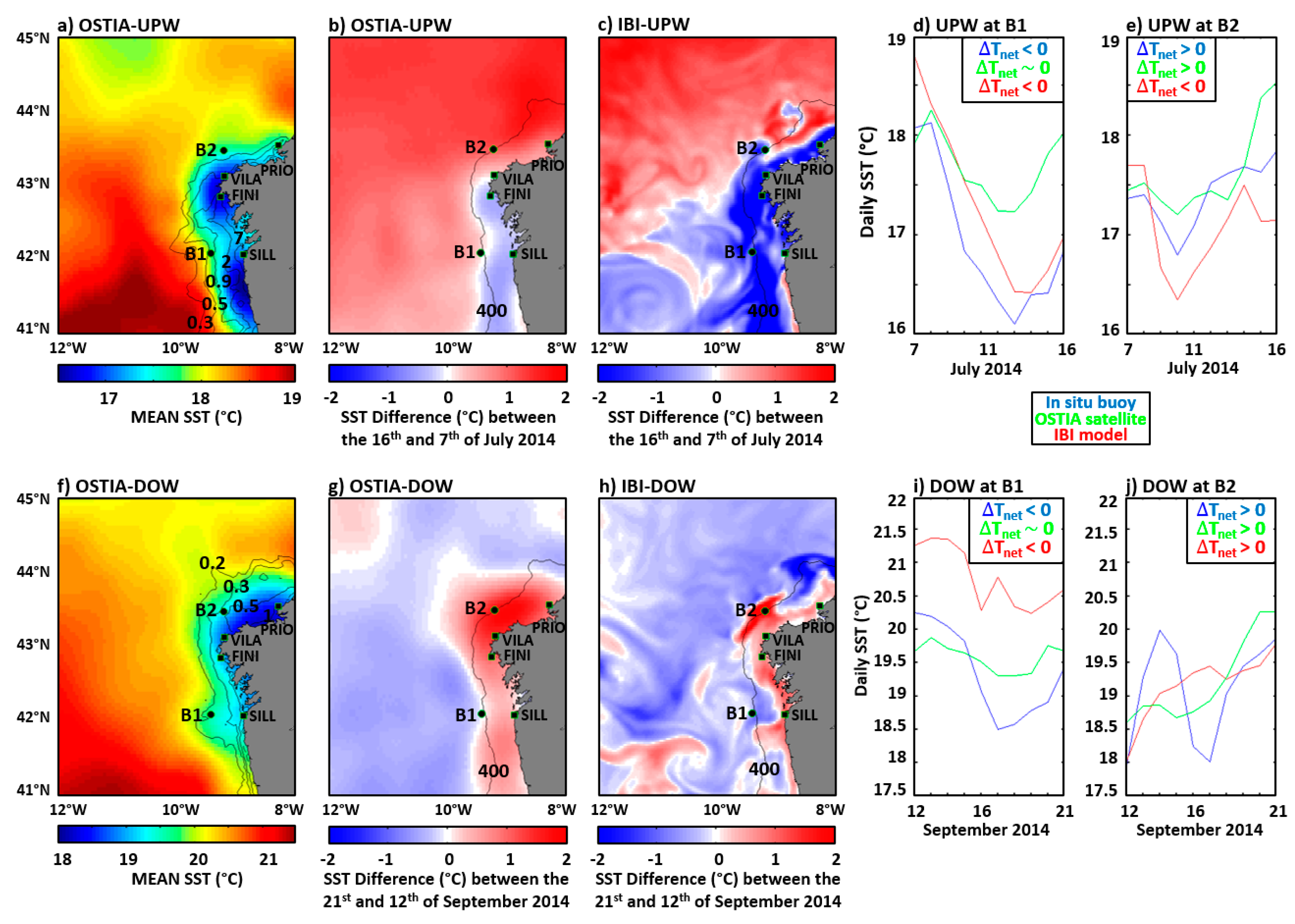
3.2.4. Sea Surface Temperature Analysis

The 10-day averaged map of satellite-derived SST and CHL during the UPW episode highlights the importance of the coastline orientation (Figure 8a). A marked cooling (below 17 °C) along the Western Galician Coast is evidenced, with surrounding warmer waters reaching up to 19 °C. Two main cores of lower SST can be observed: one located to the south of the Rias Baixas and the second one in the vicinity of CF. Isolines of constant CHL exhibit a spatial distribution in concordance with thermal fronts location. Peaks of CHL (above 7 mg·m⁻³) are detected close to the western shoreline, thus suggesting accrued injection of subsurface nutrients. By contrast, the sea surface in the Northern Galician shelf is warmer (around 17.5 °C) and not so nutrient-rich, with lower CHL concentrations, lying between 0.2 and 0.5 mg·m⁻³. These results underline the importance of the coastal orientation and confirm that stronger UPW conditions are developed in the western coast of the NW Iberian system, in concordance with References [9,10].

In order to analyze the SST evolution during the 10-day UPW event, the SST difference between the end and the beginning of such episode was explored by means of OSTIA satellite estimations (Figure 8b) and IBI model outputs (Figure 8c). Both share similarities like the overall summer warming in open-waters or the signal of upwelled waters (cooler than the original surface water), represented by a characteristic band of low SST close to the western coast. However, discrepancies arise in the intensity of the wind-driven cooling, which is broader and more intense in the case of IBI (|ΔT| > 2 °C), extended along the northern shelf in the form of a narrow strip of cool water. On the contrary, remote-sensed estimations indicate a general and relevant warming north of VILA radar site (Figure 8b). An additional difference in the modelled SST is the offshore cooling (Figure 8c), probably related to southern cyclonic recirculation cell (Figure 4b), that is absent from OSTIA map (Figure 8b).

As OSTIA is a satellite-derived product with intrinsic uncertainties, we also used in situ SST observations from B1 and B2 buoys as a reference benchmark to elucidate unequivocally the magnitude of SST variations during the two wind-induced events here analyzed. Since OSTIA is a daily satellite product, hourly estimations from IBI and both buoys were daily averaged, to gain consistency in the data sampling.

As shown in Figure 8d, in situ observations at B1 (represented by a blue line) exhibit a steep temperature decrease of 2 °C, followed by a slight recovery by the end of the UPW event, with a related net cooling of 1.5 °C. The modelled SST at the closer grid point (red line), albeit exposing a positive daily bias, is in clear qualitative accordance with in situ observations in terms of temporal evolution and net decrease of SST under UPW conditions. However, OSTIA estimations at the B1 location (green line) show a moderate drop of 1 °C and a marked recovery until reaching back the pre-UPW conditions (18 °C), in accordance with the whitish color around B1 in Figure 8b. In situ observations provided by B2 reveal a slight cooling of 0.5 °C and a gradual warming during the rest of the episode that led to a positive gradient in temperature (blue line in Figure 8e). Nevertheless, IBI outputs show a sharper decrease of 1.3 °C, followed by a water heating of 1 °C and an eventual small SST drop, yielding a final negative balance of 0.5 °C. This is already shown in Figure 8c, where the high resolution of IBI can effectively resolve sub-mesoscale dynamics like meanders and the intrusion of UPW filaments off shelf, like the one detached from the coast and presumably wrongly extended northward beyond B2 location. OSTIA estimations (green line) barely captured the SST decrease at the first stage of the UPW event, experiencing later a significant warming until 18.5 °C. Despite such a positive bias, satellite-derived estimations could replicate (and slightly overestimate) the overall warming at B2 location.

Under DOW conditions, the core of lowest SST (below 18 °C) was confined close to the Northern Galician Coast, wrapped in a strip of warmer waters (around 19.5 °C) that expanded southwestward over the shelf, far beyond B1 location (Figure 8f). The concentration of CHL revealed a significantly lower nutrient fertilization of surface waters, with isolines closer to the western shoreline but, by contrast, more distantly spaced from the northern coast, where a peak of chlorophyll (1 mg·m⁻³) was detected. By comparing the 10-day averaged maps obtained for UPW (Figure 8a) and DOW (Figure 8f), it can be readily deduced that thermal fronts (i.e., zones with a pronounced horizontal SST gradient) are often associated with higher biological productivity in coastal regions. Such a relationship between front structures and CHL concentration has been previously documented [64,65].

The SST evolution during the DOW episode was also investigated with OSTIA satellite estimations (Figure 8g) and IBI model outputs (Figure 8h). Again, the resemblance between both maps is relevant, with an overall SST increment in coastal areas, ranging from 0.5 to 2 °C. In the case of OSTIA, the warming is smoothly extended over the entire continental shelf and expose a vast peak of 2 °C in the northernmost region, surrounding B2 buoy location (Figure 8g). By contrast, IBI exhibits a narrow belt of warmer waters, confined in shallower coastal areas. A significant increase of SST (above 2 °C) is detected over the edge of the continental break, just in the periphery of B2 buoy location and detached from the coast (Figure 8h). Moreover, note that IBI seems to indicate a cooling in the close vicinity of B1, whereas OSTIA estimations reveal no substantial SST trend in that place (Figure 8g). The daily SST evolution registered at B1 buoy exhibits a net decrease of temperature, with an abrupt drop of 2 °C during the first days and a moderate recovery afterward (blue line, Figure 8i). The IBI model (red line), despite the observed bias (1 °C) in the daily outputs at the grid point closer to B1 emplacement, seems to properly resolve the overall cooling of 1 °C during the DOW event. On the contrary, OSTIA estimations scarcely captured the SST drop and the subsequent warming, reflecting a negligible SST variation between the first and the last day of the analyzed DOW episode. The situation at B2 location was, conversely, rather different (Figure 8j). The SST collected at B2 (blue line) experienced an abrupt increase, followed by an equivalent sharp drop and again by an eventual increase of almost 2 °C. The IBI model (red line) failed to capture those oscillations but agreed to reproduce adequately the net warming, with rather similar initial and final SST values. This time, OSTIA remote estimations properly reproduced the ocean water heating, despite the water temperature overestimation by the end of the event.

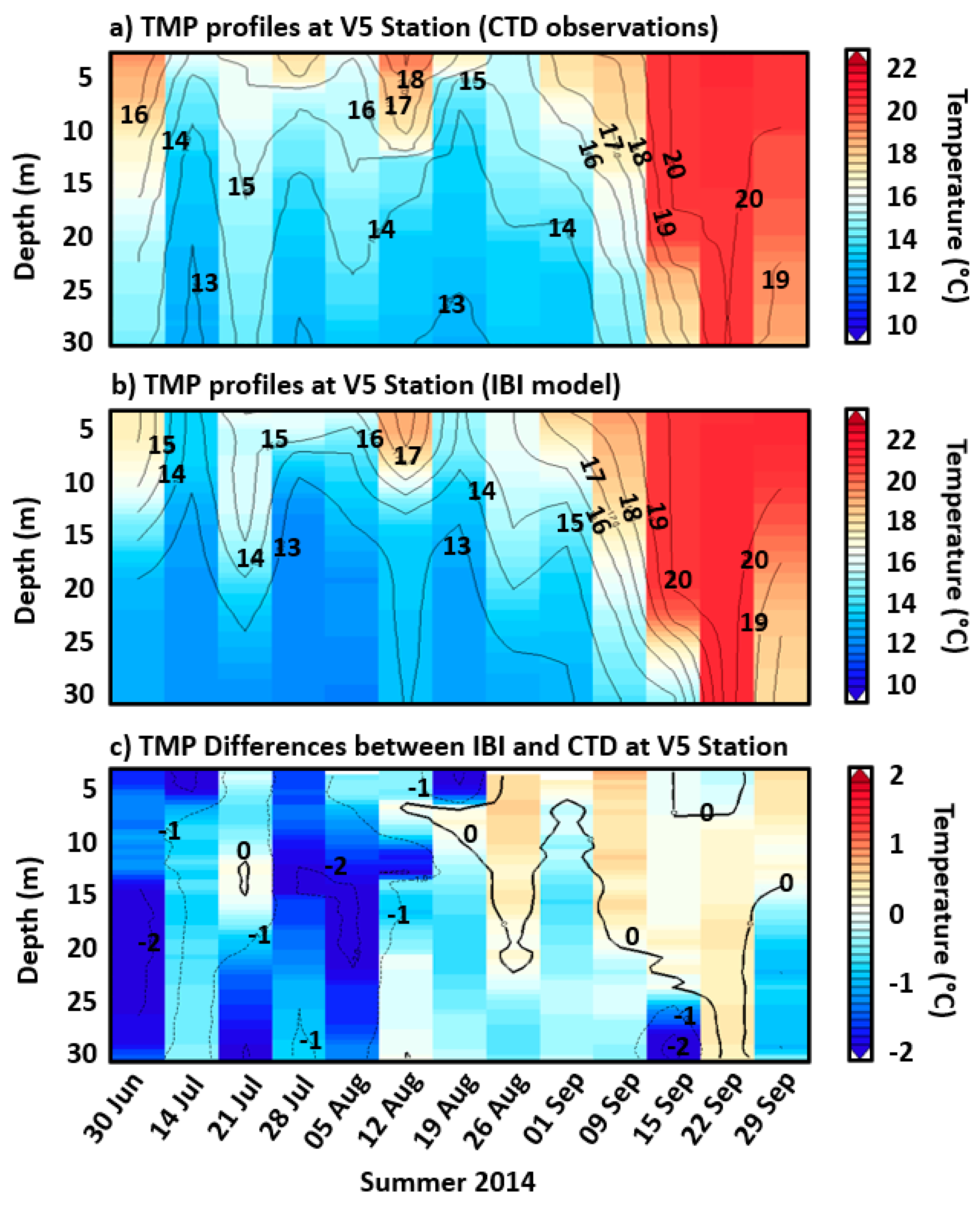
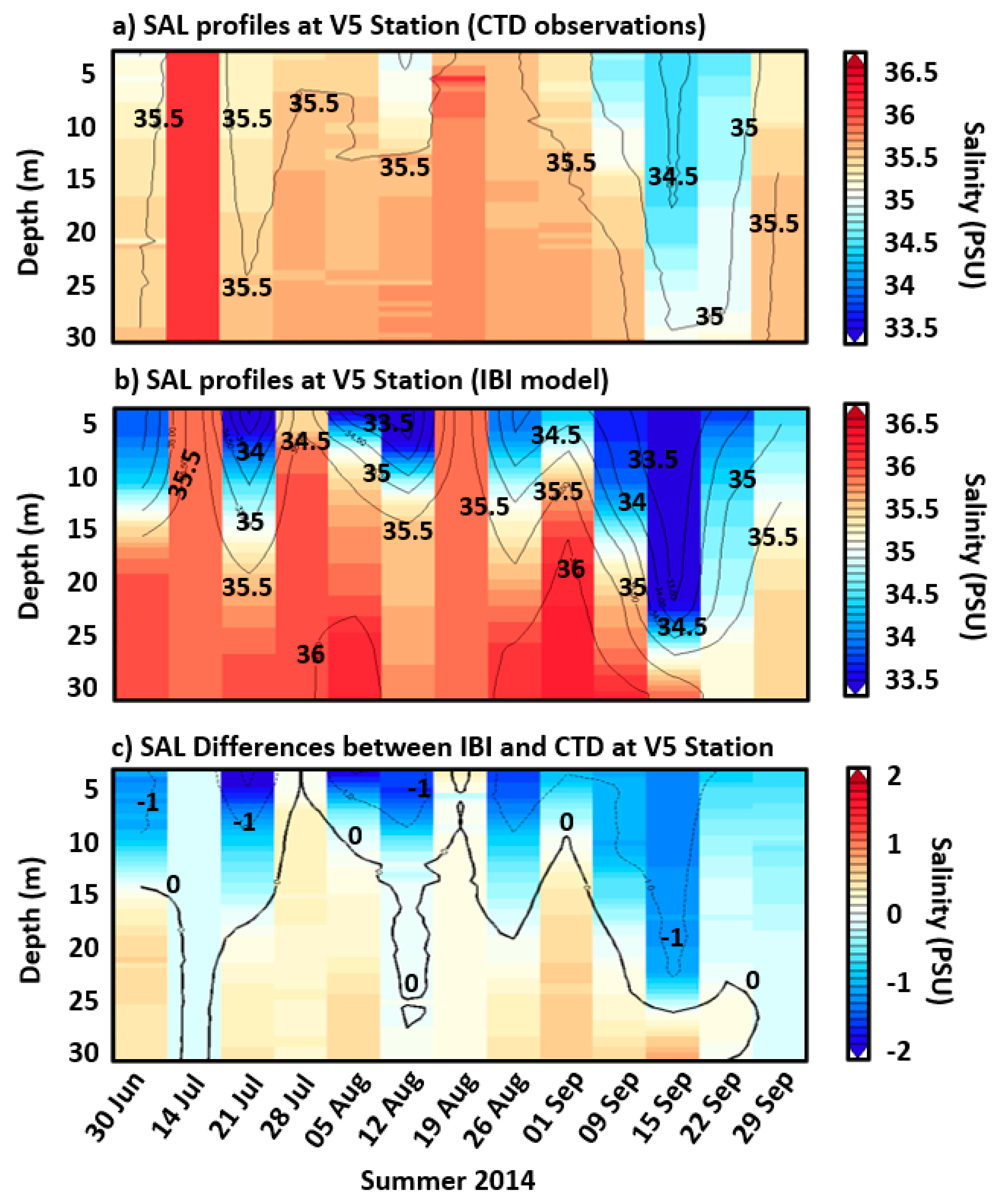
3.2.5. Vertical Analysis

In this section, the IBI model outputs were compared against independent (i.e., not assimilated) profiles of temperature and salinity, collected during the entire summer 2014, at one CTD station deployed inside of Rias Baixas (V5, denoted in Figure 1b), with the aim of portraying the vertical structure and gaining an improved insight into the three-dimensional flow geometry under UPW and DOW conditions. To this aim, IBI daily estimations at the closest grid point were used.

As shown in Figure 9a,b, the IBI–CTD accordance in the temporal evolution of the temperature field is relevant. The IBI performance appears to be sound in terms of timing, intensity and vertical extension of successive water-cooling and -warming episodes, likely related to the alternation of wind-driven UPW and DOW conditions, respectively. Especially relevant is the increase of temperature by the second half of September, where the subduction of warmer waters (20 °C) reached 30 m in depth. The agreement between CTD observations and IBI estimations, in terms of onset, strength and duration of this DOW event, is significantly high, as reflected by the moderate differences, evidenced in Figure 9c. By contrast, higher discrepancies can be observed in July 2014 when the main UPW event analyzed here took place. Negative differences seem to indicate that IBI overestimated the vertical uplift of colder waters (Figure 9c).

With regards to the salinity field (Figure 10), the model appeared to overrate the noticeable intrusion of fresher (33.5 PSU) waters into deeper levels (up to 25 m depth), related to downward motions under dominant southerly wind conditions (Figure 10b). However, IBI properly captured the upward flux of deep, dense and saltier (35.5 PSU) waters into the sea surface for several dates (14th and 28th of July, and 19th of August) coincident with UPW-favorable events, as indicated by the negligible differences observed in Figure 10c.

In order to get a more realistic diagnosis of IBI three-dimensional performance, instead of computing the bias (where positive and negative differences might partially cancel each other, leading to a more benevolent skill score), the mean absolute difference (MAD), vertically averaged over the entire study period, was used. A MAD of 0.79 °C (0.48 PSU) was derived from the IBI–CTD comparison for the temperature and salinity fields, respectively. Similar qualitative results were recently reported by Reference [66] during a validation experiment of a MOHID modelling suite against V5 CTD station.

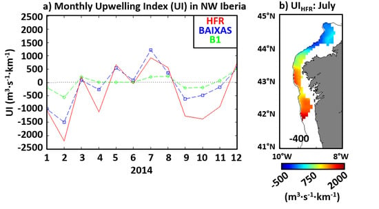
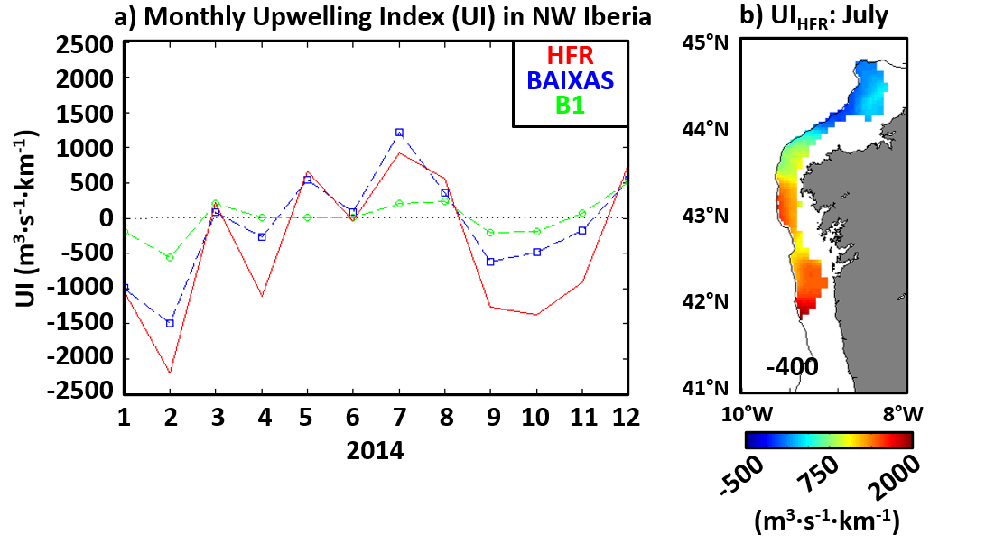
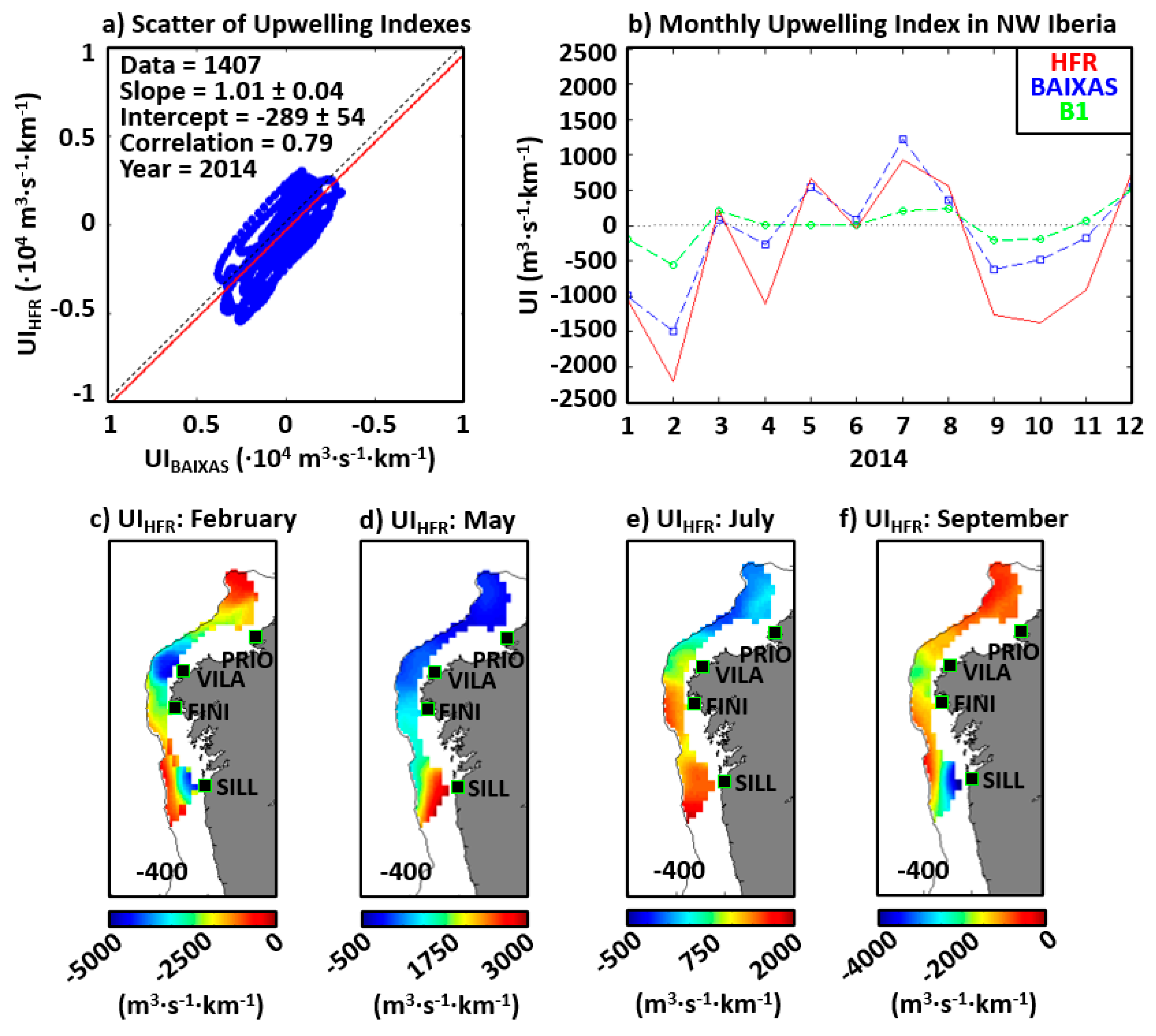
3.3. New HFR-Derived Upwelling Index: UI_HFR

In order to assess the consistency of the proposed UI_HFR, an annual validation against two preexisting coastal UIs was conducted for the entire 2014. According to the best linear fit of scatterplot between UI_HFR y UI_BAIXAS, the agreement between this novel ocean-based index and UI_BAIXAS seemed to be significantly high (Figure 11a). The slope and the correlation coefficient were close to 1 and 0.8, respectively. The comparison against UI_B1 (not shown) revealed a moderate agreement, with a lower correlation coefficient (0.49).

The temporal evolution of monthly averaged UIs showed that UI_HFR could appropriately reproduce the annual cycle along 2014, with a predominant UPW phase during the central part of the year (May–July) and prevailing DOW-favorable conditions during the rest of the months (Figure 11b). The visual resemblance with UI_BAIXAS is noticeable, although UI_HFR appears to generally overestimate the intensity of DOW scenarios. In contrast, the accordance with UI_B1 was substantially lower despite the similar evolution.

The spatial distribution of the monthly UI_HFR values exhibited recurrent features over the Galician continental shelf (Figure 11c–f). During DOW-favorable months, this coastal index persistently reached two localized minimums in the periphery of SILL and VILA radar sites. In February, UI_HFR dropped to −4800 m³·s⁻¹·km⁻¹ (Figure 11c). In September, it only decreased until −3900 m³·s⁻¹·km⁻¹ in the vicinity of SILL site. A secondary minimum, less intense (about −2000 m³·s⁻¹·km⁻¹), was detected in northern areas, around the VILA site (Figure 11f). By contrast, a prominent peak of UI_HFR (~3000 m³·s⁻¹·km⁻¹) was confined in the southernmost region under UPW-favorable conditions in May (Figure 11d). Later, a dipole-like structure was observed in July (Figure 11e), with two main cores of maximum UI_HFR (close to 2000 m³·s⁻¹·km⁻¹). Since both cores were coincident with each center of cooler and fertilized water previously evidenced in the satellite-derived SST and CHL map (Figure 8a), these results seem to confirm the viability of the proposed HFR-derived index.

With the purpose of gaining further insight into the capabilities of the new UI_HFR, we selected a variety of UPW and DOW events of diverse duration and strength, during summer 2014, and later characterized them by means of IROS metric. During July, the evolution of the three UIs shared some similarities (Figure 12a): three UPW episodes were clearly evidenced (persistently positive UI magnitudes), while a short and more elusive DOW event was categorized according to UI_BAIXAS and UI_B1 negative values. Both the time-averaged surface circulation and the spatial distribution of IROS under UPW conditions presented common peculiarities (Figure 12b,c,e). A prominent peak of IROS was clearly evidenced along the northern shallower coastal waters, expanding westward offshore in the form of a longitudinal belt (Figure 12b,c). As a result of a temporal outage that affected the northern HFR sites, the spatial coverage was substantially reduced during the last part of the month (Figure 12e). However, the strip of higher IROS values was still partially observable. By contrast, the surface circulation and IROS patterns related to the short DOW episode were kind of noisy (Figure 12d).

During August 2014, the resemblance between the three different Uis was again noticeable (Figure 13a). A relevant peak of UPW (above 4000 m³·s⁻¹·km⁻¹) was captured by each UI, although UI_HFR indicated not only more intense UPW conditions but also anticipated in the timeline. Four different episodes were eventually categorized. The first one, comprised between the 11th and 14th of August, was chosen according to high UI_HFR values, while the other remaining indexes indicated weak UPW or even DOW conditions. However, the time-averaged map of surface currents confirmed the typical offshore deflection of the flow, associated with UPW-favorable conditions (Figure 13b). Equally, we could get a glimpse of the aforementioned belt of high IROS magnitudes between FINI and VILA sites, despite the limited areal coverage. Two additional UPW events were selected, and the resulting time-averaged maps revealed similar characteristics in terms of surface circulation and IROS distribution (Figure 13c,e), in spite of the different time span (nine days versus two days). Again, a rather noisy circulation map was obtained under DOW conditions (Figure 13d), although a longitudinal belt of high IROS values was still present between FINI and VILA sites. These peculiarities were in clear accordance with the previous DOW event analyzed in July (Figure 12d).

During September 2014, the three indexes generally looked alike (Figure 14a) and jointly identified a relatively weak two-day DOW episode (days five and six). The associated circulation pattern depicted the well-documented poleward flow (Figure 14b). A delimited peak of IROS was observed, confined in coastal areas between FIST and VILA sites. A strong DOW event was classified according to the extremely persistent negative values of UI_HFR and UI_BAIXAS (around −6000 m³·s⁻¹·km⁻¹). Again, the surface waters flowed northward with higher IROS values detected over the shelf break and the NW sector (Figure 14c). Between the 22nd and 25th of September, UI_BAIXAS and UI_B1 indicated the existence of predominant UPW conditions, in opposition to UI_HFR, which simply denoted a steady relaxation of DOW until reaching a calm state (Figure 14a). The related circulation pattern indeed exhibited a prevailing poleward flow over the shelf, whereas a cyclonic recirculation could be observed in the southernmost sector of the HFR domain, likely induced by northerly winds that started to constantly blow (Figure 14d). Finally, a brief DOW event (27–28 of September) was selected according to UI_HFR negative values, although the other two indexes reflected calm conditions. The associated map of surface currents confirmed the validity of the proposed ocean-based index: The flow was effectively oriented to the north, and an elongated strip of high IROS values was encountered along the shelf break (Figure 14e).

4. Discussion

According to the results derived from the annual comparison of filtered HFR hourly time series against independent in situ current observations (Figure 2), it can de concluded that the HFR system performance was reliable for 2014, operating within suitable ranges and in line with the typical values previously reported in the literature (Table 3). RMSE (correlation) values were lower (higher) for the zonal velocity component than for the meridional: 5.72 cm·s⁻¹ vs. 8.59 cm·s⁻¹ (0.74 vs. 0.53). To some extent, such disparity might be due to the geometry of the HFR system where the site closest to B1 buoy, SILL, is installed at almost the same latitude (42°N in Figure 1b). Thus, SILL’s electromagnetic signal was the strongest over the B1 location and provided reliable radial currents, moving toward or away from the site in the latitudinal west–east axis.

Detected differences between HFR and CM current time series could be, in part, attributed a number of relevant elements, as indicated by References [67,68]: (i) sensors’ limitations (and the related instrumental noise); (ii) mismatch in the horizontal sampling (HFR provided current estimations spatially averaged over extensive areas, whereas PC gave point measurements); (iii) disparity in the depth sampling (HFR estimations were vertically integrated and representative of the upper 2 m of the water column, while CM collected at a specific 3.5 m deeper level); (iv) variations in the mixed layer and thermohaline stratification (that might impact on the vertical shear of ocean currents, especially in summertime when the two selected UPW and DOW events occurred).

The inspection of the time-averaged surface circulation patterns unveiled that the HFR adequately resolved well-known oceanographic aspects of UPW and DOW processes in the Galician Coast, such as the prevailing southwestward flow or the settlement of the poleward IPC along the NW Iberian shelf edge, respectively [7,8,9,10,11,12,13,14,15,16,17]. Equally, modelled currents appeared to reproduce satisfactorily the large-scale surface dynamics for both episodes, in close qualitative agreement with HFR-derived maps (Figure 4b,e). The correspondence was higher in regions near the shoreline, with CC coefficients generally exceeding 0.7 (Figure 4c,f). In terms of overall skill metrics (Table 4) that were spatially averaged over the common domain, the CC, zonal and meridional correlation coefficients were 0.50, 0.51 and 0.44 (0.50, 0.51 and 0.42) under UPW (DOW) conditions, respectively. These magnitudes are similar to those documented in earlier works focused on HFR-model comparisons [59,60,69] and provide added confidence in both the approach adopted and the quantitative consistency of the IBI model. Over the Galician continental shelf, model performance was even better for both the zonal and the meridional current velocities: Higher correlations and lower RMSE emerged in the ranges (0.58–0.66) and (8.26–11.87) cm·s⁻¹, respectively. In summary, the accuracy of IBI to portray the surface dynamics was not only acceptable but also similar for the UPW and DOW episodes.

The principal IBI–HFR differences stemmed from the existence of two southern cyclonic recirculation cells in the modelled currents under UPW and DOW conditions (Figure 4b,e). This is likely attributable to the significantly higher horizontal resolution of IBI, which is based on an eddy-resolving NEMO model application ($~$3 km versus 6 km). Moreover, Reference [20] previously opened the debate over the convenience or not of imposing a search radius of 25 km (already mentioned in Section 2.1) to estimate HFR total current vectors that presumably might lead to an oversmoothness of the surface circulation field. This is particularly true in the NW Iberian waters, where coastal meanders and migratory eddies have been documented to exist and have ecological implications as nutrient conveyors [70,71]. In this context, previous studies demonstrated that small-scale coastal processes are poorly reproduced (or even misrepresented) in coarser grid meshes, suggesting the strong necessity of finer horizontal resolution in both hydrodynamic models [72] and HFR systems [46] to properly capture such littoral phenomena. Since this topic remains open and disputable, further investigations should be conducted to shed light on it.

Analysis of surface divergence and vorticity fields from both IBI and HFR datasets corroborated not only the key role of the Galician shoreline orientation in modulating UPW conditions but also the importance of CF promontory and its ambient waters as a locus of permanent positive vorticity and surface divergence, independently of the dominant along-shore wind regime (Figure 5). IBI was apparently successful at reproducing broad-scale features of the HFR-derived patterns of divergence and vorticity. To the authors’ knowledge, this is the first attempt to characterize UPW and DOW conditions in the Galician waters by means of divergence and vorticity fields derived from both hourly modelled and remote-sensed surface currents. Similar initiatives were effectively addressed in the west coast of the USA [26,27,29], also identifying localized areas of positive divergence at the tip of headlands, such as Point Loma [26] or Point Reyes [27] in California, that ultimately induced topographic upwelling. With regards to the main discrepancies between the modelled and observed vorticity, they were identified in the southern sector of the common spatial domain (Figure 5f,h). Two broad cores of positive vorticity were found in IBI outcomes, presumably associated with the coherent and elongated vortexes in the along-shore direction previously described (Figure 4b,e). Over the rest of the domain, the IBI–HFR correspondence was fairly good.

Spatially averaged MKE was computed as an ancillary indicator of the temporal variability of the flow during the selected UPW and DOW periods (Figure 6). Although IBI statistically reproduced the daily evolution of MKE, the overall kinetic energy of the modelled currents was lower, indicating that a fraction of the total flow variance was not entirely replicated. Similar conclusions in relation to the limited kinematic content of the modelled flow were previously drawn by References [59,60]. The moderate but systematic underestimation of IBI currents energy at the uppermost level might be related to a limited representation of vertical stratification during the warm summer period. Indeed, results exposed in Section 3.2.5 of this paper seem to confirm this conjecture, as IBI tended to overestimate (in intensity and spatial extension) both the cooling and warming during the UPW and DOW episodes, respectively (Figure 9), thus driving an enhanced vertical mixing that might have partially slowed down the wind-induced currents speed.

The relationship of atmospheric forcing and flow variability was analyzed by means of CC maps between the wind collected at B1 buoy and observed and modelled surface currents (Figure 7). Results appeared to indicate a relevant sensitivity of IBI ocean forecast system to wind stresses in the Galician tidally dominated environment. A time-lagged vector correlation analysis was applied to investigate the reaction of the upper-layer circulation for a 24-hour interval (not shown). Maximum correlations (above 0.7) were found during the first four hours, illustrating that only a brief time is required for the subtidal current to establish the equilibrium with local wind, thus staying in conformity with Reference [56,73]. Once again, HFR and IBI exhibited a similar qualitative performance. Notwithstanding, results should be interpreted with caution since the spatial inhomogeneity of the wind field in Galicia has been previously suggested [10,56]. Although Reference [74] acknowledged that B1 buoy was free of possible errors in the correction of the terrain roughness and was, hence, the better station to represent ocean–atmosphere interactions at both Rias Baixas and the adjacent western shelf, local wind in the complex Northern Galician Coast may substantially differ and cause a decrease of maximum correlation between wind and surface currents.

The 10-day averaged map of satellite-derived SST and CHL during the UPW and DOW events confirmed the relevance of the Galician coastline’s shape (Figure 8). Abrupt changes in coastal orientation can induce noticeable wind stress fluctuations and, hence, different UPW conditions with subsequent biophysical implications, as here observed and previously documented by References [9,10,12,56]. Stronger upwelling, with cooler and more enriched waters, was evidenced in the Western Galician shelf [9,10].

The comparison of the SST field observed by OSTIA mission and modelled by IBI during the UPW event revealed interesting differences. Despite sharing similar features, the intensity of the wind-driven cooling was broader and more intense in the case of IBI. These results are in line with a recent work published by Reference [75] where a variety of L4 satellite-derived SST products (including OSTIA) were reported to underestimate the thermal fingerprint of strong coastal UPW, not only in the NW Iberian system but also in other regions worldwide. While performing satisfactorily over broad areas for most of the year, such products seemed to misrepresent UPW-induced abrupt temperature transitions in coastal waters. Notwithstanding, it is worth noting that both in situ and remote-sensing devices are affected by technical limitations and intrinsic uncertainties so SST observations from B1 and B2 buoys should only be considered as a close approximation of “ground truth”.

Additionally, IBI model daily outputs were compared against temperature and salinity profiles collected at one CTD station, with the aim of gaining further insight into the three-dimensional flow geometry under UPW and DOW conditions (Figure 9 and Figure 10). Therefore, the skill metrics here presented appear to indicate that IBI represented appropriately the main signatures of the vertical thermohaline structure along summer 2014 in the intricate Rias Baixas, where the irregular coastal morphology and abrupt gradients in local bathymetry might handicap precise hydrodynamic models forecast. Focusing on the UPW event here studied (7th–16th July), we see that the results seem to suggest that IBI misrepresented, to some extent, the associated cooling, but accurately resolved the associated salinity variability. On the contrary, the model slightly overestimated the temperature of sinking water masses under persistent DOW conditions (12th–21st September), but failed to capture their salinity. Nonetheless, since this is a single isolated example, ancillary validation exercises along the Galician Coast should be performed in the future. The detected discrepancies within the Rias Baixas might be in part attributed to discordant time sampling: While CTD devices capture instantaneous pictures of the water column state, the IBI model provides daily averaged estimations that could hypothetically include high-frequency effects of a variety of coastal processes, including riverine freshwater discharges, tidal mixing or land–sea breezes.

A variety of constraint factors inherently restrict the IBI–HFR comparison and must be taken into account when interpreting the results previously exposed. Such elements encompass remote-sensor limitations and the aforementioned GDOP, discrepancies in both the depth sampling and the horizontal grid mesh, or any potential limitation in the meteorological forcing used to run IBI ocean forecasting system (which is out of the scope of the present paper but probably deserves a detailed examination elsewhere). In the same line, model comparisons against in situ buoys, satellite-derived SST products or CTD profiles are handicapped by similar idiosyncratic aspects. As data assimilation provides the integrative framework for maximizing the joint utility of observations and ocean forecasting systems, a SAM-2 assimilation scheme [76] was later incorporated in the following version of IBI system (released in April 2018). Since then, altimetry data (along-track sea-level anomalies), OSTIA SST product and CORA (Coriolis Ocean database ReAnalysis) datasets (including ARGO, gliders, drifting buoys, etc.) are routinely assimilated into IBI operational chain in order to enhance its predictive skills. Additional efforts should be also devoted to optimizing the observations-model strategy by combining HFR synoptic circulation maps and high-resolution coastal simulations. In this context, classic observing system experiments (OSEs) could be useful to evaluate the impact of assimilating HFR data on model prognostic capabilities.

With the aim of characterizing the variability of the NW Iberian UPW system, a novel and rather simple coastal UPW index was generated from HFR-derived hourly surface current estimations, the so-called UI_HFR. Assuming the prompt and direct reaction of the upper ocean layer to intense and prolonged wind forcing, we think it seemed reasonable to develop an ocean-based proxy of UPW and DOW conditions. The proposed high-frequency index was compared with two preexisting six-hourly UPW indexes for the entire 2014. Results confirmed the consistency of UI_HFR in terms of mean values and temporal variability (Figure 11a,b). The spatial distribution of UI_HFR along the Galician continental shelf was also sound (Figure 11c–f). The map of UI_HFR corresponding to July (Figure 11e) matched well with the remotely sensed SST and CHL fields associated with the 10-day UPW event (Figure 8a), confirming the existence of relevant biophysical interactions in the NW Iberian coastal UPW system.

The skill of UI_HFR to categorize and describe UPW and DOW events during summer 2014 was also qualitatively evaluated. The most intense episodes were properly captured by UI_HFR, in agreement with the other two indexes (Figure 12a, Figure 13a and Figure 14a). Discrepancies arise from relatively short events of moderate intensity: While UI_BAIXAS and UI_B1 indicated predominant DOW (Figure 12a and Figure 13a) and UPW (Figure 14a) conditions, UI_HFR appeared to contradict the formers, revealing by contrast relaxation episodes (i.e., UI_HFR values close to zero). The related time-averaged circulation maps exhibited noisy patterns with recirculation structures: While some sectors depicted a northward circulation, other areas presented a southward flow (Figure 12d and Figure 13d). This was probably due to the transient response of the sea surface dynamics to an abrupt change in the dominant wind regime. These results support the potential of the proposed UI_HFR, albeit more exhaustive investigations should be conducted to determine not only the required thresholds to accurately discriminate UPW/DOW events but also its applicability to other regions worldwide.

The IROS diagnostic was calculated for hourly HFR surface current maps and later time-averaged to investigate some aspects of the flow dynamics under specific UPW/DOW events. High values of IROS indicate potential areas for strong dispersion of passive tracers. Under UPW conditions, maps of IROS revealed a significant offshore-directed advection in the form of a longitudinal band of high values, spatially comprised between FINI and VILA sites (Figure 12 and Figure 13) where the coastal orientation abruptly changes. Under predominant northerly winds, an elevated westward dispersion of particles in this subregion is suggested, regardless of the length and intensity of the UPW episode. The analyzed events ranged from two consecutive days of moderate UI_HFR (below 500 m³·s⁻¹·km⁻¹) to 10 days of high UI_HFR (above 2000 m³·s⁻¹·km⁻¹), leading to similar IROS magnitudes and spatial distribution, as exposed in Figure 13e and Figure 12c, respectively.

Conversely, DOW events were characterized by an acceleration of the northward jet, depicting a strong poleward advection associated with high IROS values along the shelf-break, likely due to the interplay between southerly winds and local topography (Figure 14b–e). Another peak of IROS was recurrently observed in the NW sector of the HFR domain, Once again, the ocean response was similar independently of the strength and life span of the chosen DOW episodes. The selected events ranged from two consecutive days of moderately negative UI_HFR (about −700 m³·s⁻¹·km⁻¹) to 10 days of extremely negative UI_HFR (far below −5000 m³·s⁻¹·km⁻¹), yielding similar IROS magnitudes, as shown in Figure 14e,c, respectively.

In order to expand and complete the present work, future efforts should be devoted to analyze a broader number of UPW and DOW events from a Lagrangian perspective, with a focus on particle tracking, transport and dispersion processes, residence times and water renewal mechanisms. Equally, the skill assessment of HFR Lagrangian trajectories against drifting buoys should remain as a preliminary priority before addressing this topic [46,67]. An integrated HFR-model strategy could be effective to better understand the connectivity between offshore and littoral areas along with the biophysical interactions at coastal scales, especially in the vulnerable Rias Baixas ecosystem.

Finally, a question that has emerged in recent years is the role of global warming in potential variations of UPW strength and timing that could consequently affect both the delivery of nutrients into the euphotic zone and the marine fish stocks. Former researches have investigated changes on UPW trends worldwide, reporting contradictory results that are highly dependent on the region and season selected and the characteristics of the dataset used [77,78,79]. With a focus on the NW Iberian system, recent studies have hypothesized that coastal UPW will be not as effective in the future, regardless of the tendency for an intensification of both the Azores High and UPW-favorable winds [80]. The UPW imprint is expected to be less intense during the ongoing century due to the sea surface warming and the enhanced thermal stratification of the water column that might inhibit nutrients exchange through vertical mixing.

5. Conclusions

In the present contribution, the first focus was placed on the synergistic blend of multi-platform observations and the CMEMS IBI ocean forecast system, working in concert to adequately depict the main oceanographic features of two persistent UPW and DOW events in the NW Iberian coastal system during summer 2014.

Results seem to suggest that the HFR performance was sound and credible for 2014, operating within suitable ranges and providing reliable surface current estimations in near-real time that could be effectively used for coastal monitoring and the characterization of recurring UPW and DOW episodes. Furthermore, the examination of HFR-derived surface circulation patterns confirms that this land-based technology properly resolved well-known oceanographic aspects of the Galician UPW and DOW processes, in accordance with the historical literature.

The significant resemblance between observed and modelled wind-driven currents revealed the strong connectivity between offshore and coastal ecosystems and also confirmed the importance of CF promontory as a locus of stationary peak of upwelling, in agreement with previous studies. Skill metrics showed that IBI performance was quantitatively similar for both events, with a higher degree of accuracy over the continental shelf. The primary role of the predominant wind regime in the prompt modulation of surface circulation, nutrient supply and productivity in Galicia was also evidenced. Again, a considerable accordance between IBI and the HFR was revealed in terms of surface patterns of divergence and vorticity. Equally, a good agreement in the MKE evolution was also observed, despite the reduced kinematic energy of the modelled flow.

Complementarily, the skill assessment of IBI against temperature and salinity profiles collected at one CTD station inside of Rias Baixas demonstrated that the principal signatures of the vertical thermohaline structure along summer 2014 were satisfactorily captured by the model. In conclusion, IBI may be deemed as a consistent regional ocean forecast system, able to properly resolve the large-scale surface dynamics in the NW Iberian coastal system, regardless of few shortcomings, such as the overestimation of the cooling (warming) associated with UPW (DOW) conditions. The adopted approach appears to be well-founded to efficiently characterize the hydrodynamic features of the coastal circulation but also to identify ocean modelling aspects where IBI system is still susceptible to improvement in future operational versions.

The second goal of this contribution was to develop a purely ocean-based UPW index for the NW Iberian coastal system, constructed from HFR-derived hourly surface current estimations (UI_HFR). The proposed index was validated for 2014 against traditional indexes, based on six-hourly observations of sea level pressure (UI_BAIXAS) and wind (UI_B1). Results obtained were promising, revealing the following: (i) a noticeable concordance between UI_HFR and UB_AIXAS at different timescales; (ii) a proven ability of UI_HFR to categorize properly a wealth of relevant UPW and DOW episodes that took place during summer 2014, regardless of their length and intensity; (iii) the existing biophysical interactions in the NW Iberian coastal UPW system, hence, underlying the strong link between HFR-derived wind-induced circulation and the modulation of SST and CHL fields at the uppermost layer.

Additionally, a Eulerian diagnostic denominated IROS was computed to investigate additional features of the surface flow under UPW/DOW favorable conditions. IROS emerged as a simple useful, easily computable metric that is able to determine areas of high dispersive nature. This has direct implications for the connectivity between open ocean and littoral waters though the cross-shelf transport of pollutants and larvae communities. Equally, IROS may deliver essential information for policy-making and the timely management of search-and-rescue (SAR) operations or accidental oil spills.

References

1. Botsford, L.W.; Lawrence, C.A.; Dever, E.P.; Hastings, A.; Largier, J. Effects of variable winds on biological productivity on continental shelves in coastal upwelling systems. Deep-Sea Res. Part II 2006, 53, 3116–3140. [Google Scholar] [CrossRef]
2. Lachkar, Z.; Gruber, N. What controls biological production in coastal upwelling systems? Insights from a comparative modelling study. Biogeosciences 2011, 8, 2961–2976. [Google Scholar] [CrossRef] [Green Version]
3. Hill, A.E.; Hickey, B.M.; Shillington, F.A.; Strub, P.T.; Brink, K.H.; Barton, E.D.; Thomas, A.C. Eastern ocean boundaries coastal segment (E). In The Global Coastal Ocean, Regional Studies and Syntheses, The Sea; Robinson, A.R., Brink, K.H., Eds.; John Wiley and Sons, Inc.: New York, NY, USA, 1998; Volume 11, pp. 29–67. [Google Scholar]
4. Largier, J.L.; Magnell, B.A.; Winant, C.D. Subtidal circulation over the northern California shelf. J. Geophys. Res. 1993, 98, 18147–18179. [Google Scholar] [CrossRef]
5. Bjorkstedt, E.; Roughgarden, J. Larval transport and coastal upwelling: An application of HF radar in ecological research. Oceanography 1997, 10, 64–67. [Google Scholar] [CrossRef]
6. Pitcher, G.C.; Figueiras, F.G.; Hickey, B.M.; Moita, M.T. The physical oceanography of upwelling systems and the development of harmful algal blooms. Prog. Oceanogr. 2010, 85, 5–32. [Google Scholar] [CrossRef] [Green Version]
7. deCastro, M.; Gómez-Gesteira, M.; Álvarez, I.; Lorenzo, M.; Cabanas, J.M.; Prego, R.; Crespo, A.J.C. Characterization of fall-winter upwelling recurrence along the Galician western coast (NW Spain) from 2000 to 2005: Dependence on atmospheric forcing. J. Mar. Syst. 2008, 72, 145–158. [Google Scholar] [CrossRef]
8. Torres, R.; Barton, E.D. Onset and development of the Iberian poleward flow along the Galician coast. Cont. Shelf Res. 2006, 26, 1134–1153. [Google Scholar] [CrossRef] [Green Version]
9. Álvarez, I.; Gómez-Gesteira, M.; deCastro, M.; Prego, R. Variation in upwelling intensity along the North-West Iberian Peninsula (Galicia). J. Atmos. Ocean Sci. 2005, 10, 309–324. [Google Scholar] [CrossRef]
10. Torres, R.; Barton, E.D.; Miller, P.; Álvarez-Fanjul, E. Spatial patterns of wind and sea surface temperature in the Galician upwelling region. J. Geophys. Res. 2003, 108, 3130. [Google Scholar] [CrossRef] [Green Version]
11. Prego, R.; Bao, R. Upwelling influence on the Galician coast: Silicate in shelf water and underlying surface sediments. Cont. Shelf Res. 1997, 17, 307–318. [Google Scholar] [CrossRef] [Green Version]
12. Álvarez, I.; Gómez-Gesteira, M.; deCastro, M.; Lorenzo, M.N.; Crespo, A.J.C.; Dias, J.M. Comparative analysis of upwelling influence between the western and northern coast of the Iberian Peninsula. Cont. Shelf Res. 2011, 31, 388–399. [Google Scholar] [CrossRef]
13. Gómez-Gesteira, M.; Moreira, C.; Álvarez, I.; deCastro, M. Ekman transport along the Galician coast (northwest Spain) calculated from forecasted winds. J. Geophys. Res. 2006, 111. [Google Scholar] [CrossRef]
14. Picado, A.; Álvarez, I.; Vaz, N.; Dias, J.M. Chlorophyll concentration along the north-western coast if the Iberian Peninsula vs. atmosphere-ocean-land conditions. J. Coast. Res. 2013, 65, 2047–2052. [Google Scholar] [CrossRef]
15. González-Nuevo, G.; Gago, J.; Cabanas, J.M. Upwelling Index: A powerful tool for marine research in the NW Iberian upwelling system. J. Oper. Oceanogr. 2014, 7, 47–57. [Google Scholar] [CrossRef]
16. Souto, C.; Gilcoto, M.; Fariña-Busto, L.; Pérez, F.F. Modeling the residual circulation of a coastal embayment affected by wind-driven upwelling: Circulation of the Ría de Vigo (NW Spain). J. Geophys. Res. 2003, 108, 3340. [Google Scholar] [CrossRef] [Green Version]
17. Barton, E.D.; Largier, J.L.; Torres, R.; Sheridan, M.; Trasviña, A.; Souza, A.; Pazos, Y.; Valle-Levinson, A. Coastal upwelling and downwelling forcing of circulation in a semi-enclosed bay: Ria de Vigo. Prog. Oceanogr. 2015, 134, 173–189. [Google Scholar] [CrossRef] [Green Version]
18. Barton, E.D.; Torres, R.; Figueiras, F.G.; Gilcoto, M.; Largier, J. Surface water subduction during a downwelling event in a semi-enclosed bay. J. Geophys. Res. Oceans 2016, 121, 7088–7107. [Google Scholar] [CrossRef] [Green Version]
19. Gilcoto, M.; Largier, J.L.; Barton, E.D.; Piedracoba, S.; Torres, R.; Graña, R.; Alonso-Perez, F.; Villacieros-Robineau, N.; De la Granda, F. Rapid response to coastal upwelling in a semienclosed bay. Geophys. Res. Lett. 2017, 44. [Google Scholar] [CrossRef] [Green Version]
20. Lorente, P.; Piedracoba, S.; Álvarez-Fanjul, E. Validation of high-frequency radar ocean surface current observations in the NW of the Iberian Peninsula. Cont. Shelf Res. 2015, 92, 1–15. [Google Scholar] [CrossRef]
21. Lorente, P.; Sotillo, M.G.; Aouf, L.; Amo-Baladrón, A.; Barrera, E.; Dalphinet, A.; Toledano, C.; Rainaud, R.; De Alfonso, M.; Piedracoba, S.; et al. Extreme Wave Height Events in NW Spain: A Combined Multi-Sensor and Model Approach. Remote Sens. 2018, 10, 1. [Google Scholar] [CrossRef] [Green Version]
22. Lorente, P.; Basañez Mercader, A.; Piedracoba, S.; Pérez-Muñuzuri, V.; Montero, P.; Sotillo, M.G.; Álvarez-Fanjul, E. Long-term skill assessment of SeaSonde radar-derived wave parameters in the Galician coast (NW Spain). Int. J. Remote Sens. 2019, 40. [Google Scholar] [CrossRef]
23. Shkedy, Y.; Fernandez, D.; Teague, C.; Vesecky, J.; Roughgarden, J. Detecting upwelling along the central coast of California during an El Niño year using HF radar. Cont. Shelf Res. 1995, 15, 803–814. [Google Scholar] [CrossRef]
24. Shulman, I.; Anderson, S.; Rowley, C.; DeRada, S.; Doyle, J.; Ramp, S. Comparisons of upwelling and relaxation events in the Monterrey Bay area. J. Geophys. Res. 2010, 115. [Google Scholar] [CrossRef]
25. Ramp, S.R.; Paduan, J.D.; Shulman, I.; Kindle, J.; Bahr, F.L.; Chavez, F. Observations of upwelling and relation events in the northern Monterrey Bay during August 2000. J. Geophys. Res. 2005, 110. [Google Scholar] [CrossRef]
26. Roughan, M.; Terril, E.J.; Largier, J.L.; Otero, M. Observations of divergence and upwelling around Point Loma, California. J. Geophys. Res. 2005, 110. [Google Scholar] [CrossRef] [Green Version]
27. Kaplan, D.M.; Largier, J.L. HF radar-derived origin and destination of surface waters off Bodega Bay, California. Deep-Sea Res. II 2006, 53, 2906–2930. [Google Scholar] [CrossRef]
28. Enriquez, A. An Investigation of Surface Current Patterns Related to Upwelling in Monterrey Bay, Using High Frequency Radar. Ph.D. Thesis, Naval Postgraduate School, Monterey, CA, USA, 2004. [Google Scholar]
29. Paduan, J.D.; Cook, M.S.; Tapia, V.M. Patters of upwelling and relaxation around Monterrey Bay based on long-term observations of surface currents from High Frequency radar. Deep-Sea Res. II 2018, 151, 129–136. [Google Scholar] [CrossRef]
30. Rubio, A.; Mader, J.; Corgnati, L.; Mantovani, C.; Griffa, A.; Novellino, A.; Quentin, C.; Wyatt, L.; Schulz-Stellenfleth, J.; Horstmann, J.; et al. HF Radar Activity in European Coastal Seas: Next Steps Towards a Pan-European HF Radar Network. Front. Mar. Sci. 2017, 20. [Google Scholar] [CrossRef] [Green Version]
31. Roarty, H.; Cook, T.; Hazard, L.; George, D.; Harlan, J.; Cosoli, S.; Wyatt, L.; Fanjul, E.A.; Terrill, E.; Otero, M.; et al. The Global High Frequency Radar network. Front. Mar. Sci. 2019, 14. [Google Scholar] [CrossRef]
32. De Mey-Frémaux, P.; Ayoub, N.; Barth, A.; Brewin, R.; Charria, G.; Campuzano, F.J.; Ciavatta, S.; Cirano, M.; Edwards, C.; Federico, I.; et al. Model-Observations synergy in the coastal ocean. Front. Mar. Sci. 2019, 6. [Google Scholar] [CrossRef] [Green Version]
33. Davidson, F.; Alvera-Azcárate, A.; Barth, A.; Brassington, G.B.; Chassignet, E.P.; Clementi, E.; De Mey-Frémaux, P.; Divakaran, P.; Harris, C.; Hernandez, F.; et al. Synergies in Operational Oceanography: The intrinsic need for sustained ocean observations. Front. Mar. Sci. 2019, 6. [Google Scholar] [CrossRef] [Green Version]
34. Le Traon, P.Y.; Ali, A.; Álvarez-Fanjul, E.; Aouf, L.; Axell, L.; Aznar, R.; Ballarotta, M.; Behrens, A.; Mounir, B.; Bentamy, A.; et al. The Copernicus Marine Environmental Monitoring Service: Main Scientific Achievements and Future Prospects. Mercator Ocean J. 2017, 56, 1–101. [Google Scholar]
35. Barrick, D.E.; Lipa, B.J. Correcting for distorted antenna patterns in CODAR ocean surface measurements. IEEE J. Oceanic Eng. 1986, 11, 304–309. [Google Scholar] [CrossRef]
36. Barrick, D. Geometrical Dilution of Statistical Accuracy (GDOSA) in Multi-Static HF Radar Networks; CODAR Ocean Sensors Ltd.: Mountain View, CA, USA, 2006. [Google Scholar]
37. Madec, G. NEMO Ocean General Circulation Model, Reference Manual, Internal Report; LODYC/IPSL: Paris, France, 2008. [Google Scholar]
38. Sotillo, M.G.; Cailleau, S.; Lorente, P.; Levier, B.; Aznar, R.; Reffray, G.; Amo-Baladrón, A.; Álvarez-Fanjul, E. The MyOcean IBI Ocean Forecast and Reanalysis Systems: Operational products and roadmap to the future Copernicus Service. J. Oper. Oceanogr. 2015, 8, 1–18. [Google Scholar] [CrossRef]
39. Kundu, P. Ekman veering observed near the ocean bottom. J. Phys. Oceanogr. 1976, 6, 238–242. [Google Scholar] [CrossRef]
40. Futch, V. The Lagrangian Properties of the Flow West of Oahu. Master’s Thesis, University of Hawaii, Honolulu, HI, USA, 2009. [Google Scholar]
41. Archer, M.R.; Shay, L.K.; Jaimes, B.; Martinez-Pedraja, J. Observing frontal instabilities of the Florida current using high frequency radar. In Coastal Ocean Observing Systems; Liu, Y., Kerkering, H., Weisberg, R.H., Eds.; Elsevier Inc.: Amsterdam, The Netherlands, 2015; Chapter 11; pp. 179–208. [Google Scholar] [CrossRef]
42. Schaeffer, A.; Gramoulle, A.; Roughan, M.; Mantovanelli, A. Characterizing frontal eddies along the East Australian Current from HF radar observations. J. Geophys. Res. Oceans 2017, 122, 3964–3980. [Google Scholar] [CrossRef]
43. Jacox, M.G.; Edwards, C.A.; Hazen, E.L.; Bograd, S.J. Coastal upwelling revisited: Ekman, Bakun and improved upwelling indexes for the US West Coast. J. Geophys. Res. Oceans 2018, 123, 7332–7350. [Google Scholar] [CrossRef]
44. Cosoli, S.; Mazzoldi, A.; Gacic, M. Validation of surface current measurements in the Northern Adriatic Sea from High Frequency radars. J. Atmos. Ocean. Technol. 2010, 27, 908–919. [Google Scholar] [CrossRef]
45. Robinson, A.M.; Wyatt, L.R.; Howarth, M.J. A two-year comparison between HF radar and ADCP current measurements in Liverpool Bay. J. Oper. Oceanogr. 2011, 4, 33–45. [Google Scholar] [CrossRef] [Green Version]
46. Rypina, I.I.; Kirincich, A.R.; Limeburner, R.; Udovydchenkov, I.A. Eulerian and lagrangian correspondence of High-Frequency radar and surface drifter data: Effects of radar resolution and flow components. J. Atmos. Ocean. Technol. 2014, 31, 945–966. [Google Scholar] [CrossRef] [Green Version]
47. Kohut, J.T.; Glenn, S.M. Improving HF radar surface current measurements with measured antenna beam patterns. J. Atmos. Ocean. Technol. 2003, 20, 1303–1316. [Google Scholar] [CrossRef]
48. Emery, W.J.; Thomson, R.E. Data Analysis Methods in Physical Oceanography; Elsevier Science: Amsterdam, The Netherlands, 2001; p. 654. ISBN 9780080477008. [Google Scholar]
49. Alfonso, M.; Álvarez-Fanjul, E.; López, J.D. Comparison of CODAR SeaSonde HF Radar Operational Waves and Currents Measurements with Puertos del Estado Buoys; Final Internal Report of Puertos del Estado: Madrid, Spain, 2006; pp. 1–32. [Google Scholar]
50. Rubio, A.; Reverdin, G.; Fontán, A.; González, M.; Mader, J. Mapping near-inertial variability in the SE Bay of Biscay from HF radar data and two offshore moored buoys. Geophys. Res. Lett. 2011, 38, L19607. [Google Scholar] [CrossRef]
51. Solabarrieta, L.; Rubio, A.; Castanedo, S.; Medina, R.; Charria, G.; Hernández, C. Surface water circulation patterns in the southeastern Bay of Biscay: New evidences from HF radar data. Cont. Shelf Res. 2014, 74, 60–76. [Google Scholar] [CrossRef] [Green Version]
52. Lorente, P.; Piedracoba, S.; Soto-Navarro, J.; Álvarez-Fanjul, E. Accuracy assessment of high frequency radar current measurements in the Strait of Gibraltar. J. Oper. Oceanogr. 2014, 7, 59–73. [Google Scholar] [CrossRef]
53. Lana, A.; Marmain, J.; Fernández, V.; Tintoré, J.; Orfilia, A. Wind influence on surface current variability in the Ibiza Channel from HF Radar. Ocean Dyn. 2016, 66, 483–497. [Google Scholar] [CrossRef]
54. Mihanović, H.; Cosoli, S.; Vilibić, I.; Ivanković, D.; Dadić, V.; Gačić, M. Surface current patterns in the northern Adriatic extracted from high-frequency radar data using self-organizing map analysis. J. Geophys. Res. 2011, 116. [Google Scholar] [CrossRef] [Green Version]
55. Gačić, M.; Kovačević, V.; Cosoli, S.; Mazzoldi, A.; Paduan, J.D.; Mancero-Mosquera, I.; Yari, S. Surface current patterns in front of the Venice Lagoon. Estuar. Coast. Shelf Sci. 2009, 82, 485–494. [Google Scholar] [CrossRef]
56. McClain, C.R.; Chao, S.Y.; Atkinson, L.P.; Blanton, J.O.; Decastillejo, F. Wind-Driven Upwelling in the Vicinity of Cape Finisterre, Spain. J. Geophys. Res.-Ocean. 1986, 91, 8470–8486. [Google Scholar] [CrossRef] [Green Version]
57. Teles-Machado, A.; Peliz, A.; McWilliams, J.C.; Cardoso, R.M.; Soares, P.M.M.; Miranda, P.M.A. On the year-to-year changes of the Iberian Poleward Current. J. Geophys. Res. Oceans 2015, 120. [Google Scholar] [CrossRef]
58. Otero, P.; Ruiz-Villareal, M.; Peliz, A. Variability of river plumes off Northwest Iberia in response to wind events. J. Mar. Syst. 2008, 72, 238–255. [Google Scholar] [CrossRef]
59. O’Donncha, F.; Hartnett, M.; Nash, S.; Ren, L.; Ragnoli, E. Characterizing observed circulation patterns within a bay using HF radar and numerical model simulations. J. Mar. Syst. 2015, 142, 96–110. [Google Scholar] [CrossRef]
60. Cosoli, S.; Licer, M.; Vodopivec, M.; Malacic, V. Surface circulation in the Gulf of Trieste (northern Adriatic Sea) from radar, model, and ADCP comparisons. J. Geophys. Res. Oceans 2013, 118, 6183–6200. [Google Scholar] [CrossRef]
61. Aguiar, E.; Mourre, B.; Juza, M.; Reyes, M.; Hérnandez-Lasheras, J.; Cutolo, E.; Mason, E.; Tintoré, J. Multi-platform model assessment in the Western Mediterranean Sea: Impact of downscaling on the surface circulation and mesoscale activity. Ocean Dyn. 2020, 70, 273–288. [Google Scholar] [CrossRef] [Green Version]
62. Cosoli, S.; Gacic, M.; Mazzoldi, A. Surface current variability and wind influence in the north eastern Adriatic Sea as observed from high-frequency (HF) radar measurements. Cont. Shelf Res. 2012, 33, 1–13. [Google Scholar] [CrossRef]
63. Lee, S.H.; Kang, C.Y.; Choi, B.J.; Kim, C.S. Surface Current Response to Wind and Plumes in a Bay-shape Estuary of the eastern Yellow Sea: Ocean Radar Observation. Ocean Sci. 2013, 48, 117–139. [Google Scholar] [CrossRef]
64. Stegmann, P.M.; Ullman, D.S. Variability in Chlorophyll and Sea Surface Temperature Fronts in the Long Island Sound Outflow Region from Satellite Observations. J. Geophys. Res. Oceans 2004, 109. [Google Scholar] [CrossRef] [Green Version]
65. Ye, H.; Kalhoro, M.A.; Morozov, E.; Tang, D.; Wang, S.; Thies, P.R. Increased chlorophyll-a concentration in the South China Sea caused by occasional sea surface temperature fronts at peripheries of eddies. Int. J. Remote Sens. 2017, 39, 4360–4375. [Google Scholar] [CrossRef]
66. Venancio, A.; Montero, P.; Costa, P.; Regueiro, S.; Brands, S.; Taboada, J. An integrated Perspective of the Operational Forecasting System in Rías Baixas (Galicia, Spain) with Observational Data and End-Users. In Computational Science, ICCS 2019, Proceedings of the 9th International Conference, Faro, Portugal, 12–14 June 2019; Springer International Publishing: Cham, Switzerland, 2019. [Google Scholar]
67. Ohlmann, C.; White, P.; Washburn, L.; Terril, E.; Emery, B.; Otero, M. Interpretation of coastal HF radar-derived currents with high-resolution drifter data. J. Atmos. Ocean. Technol. 2007, 24, 666–680. [Google Scholar] [CrossRef] [Green Version]
68. Kohut, J.; Roarty, H.J.; Glenn, S. Characterizing Observed Environmental variability with HF Doppler radar surface mappers and Acoustic Doppler Current Profilers: Environmental variability in the Coastal Ocean. J. Ocean. Eng. 2006, 31, 876–884. [Google Scholar] [CrossRef]
69. Yu, P.; Kurapov, A.L.; Egbert, G.D.; Allen, J.S.; Kosro, M. Variational assimilation of HF radar currents in a coastal ocean model off Oregon. Ocean Model. 2012, 49–50, 86–104. [Google Scholar] [CrossRef]
70. Oliveira, P.B.; Peliz, A.; Dubert, J.; Rosa, T.; Santos, A.M.P. Winter geostrophic currents and eddies in the western Iberia coastal transition zone. Deep Sea Res. I 2004, 51, 367–381. [Google Scholar] [CrossRef]
71. Peliz, A.; Santos, A.M.P.; Oliveira, P.B.; Dubert, J. Extreme cross-shelf transport induced by eddy interactions southwest of Iberia in winter 2001. Geophys. Res. Lett. 2004, 31, L08301. [Google Scholar] [CrossRef]
72. Lorente, P.; García-Sotillo, M.; Amo-Baladrón, A.; Aznar, R.; Levier, B.; Sánchez-Garrido, J.C.; Sammartino, S.; de Pascual-Collar, A.; Reffray, G.; Toledano, C.; et al. Skill assessment of global, regional, and coastal circulation forecast models: Evaluating the benefits of dynamical downscaling in IBI (Iberia–Biscay–Ireland) surface waters. Ocean Sci. 2019, 5, 967–996. [Google Scholar] [CrossRef] [Green Version]
73. Huthnance, J.M.; Van Aken, H.M.; White, M.; Barton, E.D.; LeCann, B.; Coelho, E.F.; Álvarez-Fanjul, E.; Miller, P.; Vitorino, J. Ocean margin exchange-water flux estimates. J. Mar. Syst. 2002, 32, 107–137. [Google Scholar] [CrossRef]
74. Herrera, J.L.; Piedracoba, S.; Varela, R.; Rosón, G. Spatial analysis of the wind field on the western coast of Galicia (NW Spain) from in situ measurements. Cont. Shelf Res. 2005, 25, 1728–1748. [Google Scholar] [CrossRef]
75. Meneghesso, C.; Seabra, R.; Broitman, B.R.; Wethey, D.S.; Burrows, M.T.; Chan, B.K.K.; Guy-Haim, T.; Ribeiro, P.A.; Rilov, G.; Santos, A.M.; et al. Remotely-sensed L4 SST underestimates the thermal fingerprint of coastal upwelling. Remote Sens. Environ. 2020, 237, 111588. [Google Scholar] [CrossRef]
76. Brasseur, P.; Bahurel, P.; Bertino, L.; Birol, F.; Brankart, J.M.; Ferry, N.; Losa, S.; Remy, E.; Schröter, J.; Skachko, S.; et al. Data assimilation for marine monitoring and prediction: The MERCATOR operational assimilation systems and the MERSEA developments. Q. J. R. Meteorol. Soc. 2005, 131, 3561–3582. [Google Scholar] [CrossRef] [Green Version]
77. Varela, R.; Álvarez, I.; Santos, F.; deCastro, M.; Gómez-Gesteira, M. Has upwelling strengthened along worldwide coasts over 1982–2010? Sci. Rep. 2015, 5. [Google Scholar] [CrossRef]
78. Barton, E.D.; Field, D.B.; Roy, C. Canary current upwelling: More or less? Prog. Oceanogr. 2013, 116, 167–178. [Google Scholar] [CrossRef] [Green Version]
79. García-Reyes, M.; Largier, J. Observations of increased wind-driven coastal upwelling off central California. J. Geophys. Res. Oceans 2010, 115, C04011. [Google Scholar] [CrossRef] [Green Version]
80. Sousa, M.C.; Ribeiro, A.; Des, M.; Gomez-Gesteira, M.; deCastro, M.; Dias, J.M. NW Iberian Peninsula coastal upwelling future weakening: Competition between wind intensification and surface heating. Sci. Total Environ. 2020, 703, 134808. [Google Scholar] [CrossRef] [PubMed]
Figure 1. (a) Daily sea surface temperature (SST) for the 15th of July 2014, as predicted by the Iberia––Biscay–Ireland (IBI) forecast system. Northwestern (NW) Iberian upwelling system denoted by the black box. (b) Temporal availability (%) of high-frequency radar (HFR) hourly data for 2014. Locations of Silleiro (B1) and Vilano (B2) buoys and four radar sites (Silleiro (SILL), Finisterre (FINI), Vilán (VILA) and Prior (PRIO)) are marked with a filled dot and squares, respectively. HFR network jointly managed by INTECMAR and Puertos del Estado. CF (in light blue) represents the Cape Finisterre promontory. Rías Baixas denoted by the purple box, with one tiny dark blue dot inside representing a Conductivity–Temperature–Depth (CTD) station (V5). Bathymetric contours show depths at 400 and 1500 m. (c) Spatial distribution of the Geometric Dilution of Precision (GDOP) for the geometry of the Galician HFR system. (d) Annual availability of HFR data: spatial coverage versus temporal coverage. Black dotted lines represent the recommended 80–80% level of data provision.
Remotesensing 12 02762 g001
Figure 2. Annual (2014) comparison of zonal (a,c) and meridional (b,d) hourly surface current velocities observed by B1 buoy and HFR (at the closest grid point): 30-h low-pass filtered time series (a,b) and best linear fit of scatter plots (c,d). Skill metrics gathered in black boxes.
Remotesensing 12 02762 g002
Figure 3. Wind roses, indicating predominant propagation direction at B1 buoy during July (a) and September (b) of 2014. Stick diagrams (depicted every 3 h) of hourly averaged wind during the 10-day upwelling-favorable (c) and downwelling-favorable events (d).
Remotesensing 12 02762 g003
Figure 4. Ten-day averaged surface circulation patterns during upwelling (UPW, ac) and downwelling (DOW, df) wind-driven events as observed with the high-frequency radar (HFR, a,d) and modelled by IBI ocean forecast system (b,e). The associated complex correlation (CC) index between IBI and HFR is presented (c,f). The isolines show the veering. Bold arrows indicate the predominant propagation direction of the wind registered at B1 buoy (shown in Figure 1b) during the 10-day periods.
Remotesensing 12 02762 g004
Figure 5. Ten-day averaged maps of horizontal divergence (ad) and vorticity (eh) derived from HFR and IBI model estimations during the upwelling (UPW) and downwelling (DOW) events. In lower panels (eh), black arrows show a schematic representation of the mean circulation during the analyzed episodes.
Remotesensing 12 02762 g005
Figure 6. (a) Evolution of daily mean kinetic energy (MKE) under upwelling (UPW) conditions, averaged over the shelf (solid lines) and open waters (dashed lines), derived from hourly surface currents provided by the HFR (blue color) and IBI model (red). (b) Idem, under downwelling (DOW) conditions. (c,d) Evolution of daily averaged low-pass filtered wind speed (module), derived from hourly estimations at B1 buoy, during the UPW and DOW events, respectively.
Remotesensing 12 02762 g006
Figure 7. Maps of complex correlation (CC) index between low-pass filtered hourly wind at B1 buoy and subtidal surface currents provided by the HFR (a,c) and IBI model (b,d), under upwelling (UPW, a,b) and downwelling (DOW, c,d) conditions. Black dot represents B1 buoy.
Remotesensing 12 02762 g007
Figure 8. (a) Ten-day averaged map of OSTIA-derived sea surface temperature (SST, colors) and chlorophyll concentration (CHL, isolines) for the upwelling (UPW) event comprised between the 7th and 16th July 2014. (b,c) SST differences between the end and the beginning of the UPW event, computed from OSTIA satellite and IBI model daily estimations, respectively. (d,e) Daily evolution of SST at B1 and B2 buoys location, respectively, as derived from in situ observations (blue line), OSTIA estimations (green line) and IBI model outputs (red line). (f) Ten-day averaged map of OSTIA-derived SST and CHL for the downwelling (DOW) event comprised between the 12th and 21st September 2014. (g,h) SST differences between the end and the beginning of the DOW event, computed from OSTIA satellite and IBI model daily estimations, respectively. (i,j) Daily evolution of SST at B1 and B2 buoys location, respectively, as derived from in situ observations (blue line), OSTIA estimations (green line) and IBI model outputs (red line).
Remotesensing 12 02762 g008
Figure 9. Comparison of temperature (TMP) profiles registered at V5 station (denoted in Figure 1b) by a CDT device (a) and IBI model (b) at the closest grid point. (c) Differences of TMP between the modelled and the observed profiles. Note that this figure is not a Hovmöller diagram but a temporal concatenation of specific dates: Only those CTD in situ observations that successfully fulfilled the quality control have been depicted.
Remotesensing 12 02762 g009
Figure 10. Comparison of salinity (SAL) profiles registered at V5 station (denoted in Figure 1b) by a CDT device (a) and IBI model (b) at the closest grid point. (c) Differences of SAL between the modelled and the observed profiles. Note that this figure is not a Hovmöller diagram but a temporal concatenation of specific dates: Only those CTD in situ observations that successfully fulfilled the quality control have been depicted.
Remotesensing 12 02762 g010
Figure 11. (a) Best linear fit of scatter plot between two different coastal upwelling indexes, for the entire year 2014; (b) Annual (2014) evolution of monthly-averaged coastal upwelling indexes: upwelling index based on HFR-derived hourly surface current observations (UIHFR) = red line, upwelling index based on hourly data of sea level pressure (UIBAIXAS) = blue line and upwelling index based on wind (UIB1) = green line. (cf) Spatial distribution of monthly averaged UIHFR over the Galician continental shelf under predominant DOW (c,f) and UPW (d,e) conditions. Bathymetric contour shows depth at 400 m.
Remotesensing 12 02762 g011
Figure 12. (a) Temporal evolution of hourly UIHFR (red line) and 6-hourly UIBAIXAS (blue squares) and UIB1 (green dots) during July 2014. Gray boxes indicate four selected UPW and DOW episodes; (be) Maps of time-averaged circulation and Instantaneous Rate of Separation (IROS) for each specific event. IROS magnitudes are normalized by the absolute value of the Coriolis parameter f.
Remotesensing 12 02762 g012
Figure 13. (a) Temporal evolution of hourly UIHFR (red line) and six-hourly UIBAIXAS (blue squares) and UIB1 (green dots) during August 2014. Gray boxes indicate four selected UPW and DOW episodes. (be) Maps of time-averaged circulation and Instantaneous Rate of Separation (IROS) for each specific event. IROS magnitudes are normalized by the absolute value of the Coriolis parameter, f.
Remotesensing 12 02762 g013
Figure 14. (a) Temporal evolution of hourly UIHFR (red line) and 6-hourly UIBAIXAS (blue squares) and UIB1 (green dots) during September 2014. Gray boxes indicate four selected UPW and DOW episodes. (be) Maps of time-averaged circulation and Instantaneous Rate of Separation (IROS) for each specific event. Bathymetric contour shows depth at 400 m. IROS magnitudes are normalized by the absolute value of the Coriolis parameter, f.
Remotesensing 12 02762 g014