


No CrossRef data available.
Article contents
Reply to the comments by Kochtitzky and Edwards (2020) on the study ‘Area changes of glaciers on active volcanoes in Latin America’ by Reinthaler and others (2019)
Published online by Cambridge University Press: 26 August 2020
Abstract
An abstract is not available for this content. As you have access to this content, full HTML content is provided on this page. A PDF of this content is also available in through the ‘Save PDF’ action button.
- Type
- Communication
- Information
- Creative Commons

 This is an Open Access article, distributed under the terms of the Creative Commons Attribution licence (http://creativecommons.org/licenses/by/4.0/), which permits unrestricted re-use, distribution, and reproduction in any medium, provided the original work is properly cited.
- Copyright
- Copyright © The Author(s) 2020
References
Barcaza, G and 7 others (2017) Glacier inventory and recent glacier variations in the Andes of Chile, South America. Annals of Glaciology 58(75), 166–180. doi: 10.1017/aog.2017.28.CrossRefGoogle Scholar
Braun, MH and 8 others (2019) Constraining glacier elevation and mass changes in South America. Nature Climate Change 9, 130–136. doi: 10.1594/PANGAEA.893612.CrossRefGoogle Scholar
Dussaillant, I and 8 others (2019) Two decades of glacier mass loss along the Andes. Nature Geoscience 12(10), 802–808. doi: 10.1038/s41561-019-0432-5.CrossRefGoogle Scholar
Kochtitzky, W and Edwards, B (2020) Comments on ‘Area changes of glaciers on active volcanoes in Latin America’ by Reinthaler and others (2019). Journal of Glaciology 66(257), 520–522. doi: https://doi.org/10.1017/jog.2020.25.CrossRefGoogle Scholar
Kochtitzky, W, Edwards, B, Enderlin, E, Marino, J and Marinque, N (2018) Improved estimates of glacier change rates at Nevado Coropuna Ice Cap, Peru. Journal of Glaciology 64(244), 175–184. doi: 10.1017/jog.2018.2.CrossRefGoogle Scholar
Lea, JM (2018) The Google Earth Engine Digitisation Tool (GEEDiT) and the Margin change Quantification Tool (MaQiT) – simple tools for the rapid mapping and quantification of changing Earth surface margins. Earth Surface Dynamics 6, 551–561. doi: 10.5194/esurf-6-551-2018.CrossRefGoogle Scholar
Paul, F and 10 others (2017) Error sources and guidelines for quality assessment of glacier area, elevation change, and velocity products derived from satellite data in the Glaciers_cci project. Remote Sensing of Environment 203, 256–275. doi: 10.1016/j.rse.2017.08.038.CrossRefGoogle Scholar
Rastner, P, Strozzi, T and Paul, F (2017) Fusion of multi-source satellite data and DEMs to create a new glacier inventory for Novaya Zemlya. Remote Sensing 9(11), 1122. doi: 10.3390/rs9111122.CrossRefGoogle Scholar
Winsvold, HS, Kääb, A and Nuth, C (2016) Regional glacier mapping using optical satellite data time series. IEEE Journal of Selected Topics in Applied Earth Observations and Remote Sensing 9(8), 3698–3711. doi: 10.1109/JSTARS.2016.2527063.CrossRefGoogle Scholar
Zalazar, L and 9 others (2020) Spatial distribution and characteristics of Andean ice masses in Argentina: results from the first National Glacier Inventory. Journal of Glaciology. doi: 10.1017/jog.2020.55.CrossRefGoogle Scholar
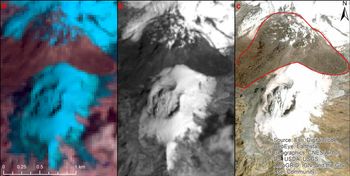
Fig. 1. Satellite scenes of the southern part of Nevado del Huila: (a) Landsat 8 from 14 January 2016: 30 m optical bands 6, 5, 4 as RGB; (b) Landsat 8 from 14 January 2016: 15 m panchromatic band 8 and (c) WorldView-2 from 28 January 2016: 0.5 m multispectral image. With the lower resolution Landsat images it is challenging to identify the newly formed lava dome marked with the red outline in (c). The distinctive texture of the lava cannot be seen at a lower resolution and thus could be misinterpreted as bare rock.
 You have
Access
You have
Access
 Open access
We appreciate the careful analysis performed by Kochtitzky and Edwards (2020). They described an overestimation of glacier area and retreat rates for the Nevado Coropuna Ice Cap and Nevado del Huila in the study by Reinthaler and others (2019), most likely due to the inclusion of seasonal snow in our glacier maps.
They nicely illustrated how large the impact can be when not using the best images available (with regards to snow conditions) and the potentially biased conclusions one might derive from a related change assessment. Their detailed investigation also illustrates that the uncertainty one can derive from theoretical concepts - such as multiple digitising of glaciers or the buffer method (e.g. Paul and others, Reference Paul2017) - are indeed only statistical measures that can be calculated, but might not represent the real issues of a dataset. In reality, the methodological uncertainties (e.g. due to adverse snow conditions or differently interpreted debris cover) can be much higher, reaching up to 50% or even more for some cases. Erroneously mapped snow cover is also a major problem for most of the glacier outlines available for the Andes in the current version 6 of the Randolph Glacier Inventory (RGI). As these outlines are used widely as an input for regional scale (hydrologic) studies or mass-balance assessments (e.g. Braun and others, Reference Braun2019; Duissallant and others, Reference Dussaillant2019), there is an urgent need to get glaciers in the entire Andes properly mapped. The latest national glacier inventories from Chile (Barcaza and others, Reference Barcaza2017) and Argentina (Zalazar and others, Reference Zalazar2020) will likely help reduce the quality issues and improve the dataset for such applications.
Although the satellite scenes used for our study have been carefully selected to avoid the snow problem, we recognise that in the case of Nevado Coropuna better images would have been available as Kochtitzky and Edwards (Reference Kochtitzky and Edwards2020) demonstrate. Nevado Coropuna has been the object of repeated erroneous mapping based on satellite images, as Kochtitzky and Edwards show in their commentary and the Kochtitzky and others (Reference Kochtitzky, Edwards, Enderlin, Marino and Marinque2018) study. They have taken great care to obtain the best possible results for their study area. However, we need to recall that our study was a regionally extensive mapping effort across Latin America, from Mexico down to Patagonia, rather than a local study with a focus on a particular mountain. Thus, for some specific locations we might have missed the best satellite scenes available. Our temporal restriction to three specific time steps (1985, 2000 and 2015 ± 1 year) had been surpassed in a few regions by several years (e.g. 1991 instead of 1985) when the other scenes available were clearly unusable. In the case a scene close to the target date was considered appropriate, further scenes were not analysed. As a consequence, the even better scenes from 1987 and 1998 for the region Coropuna were not found. We agree that it is always worth the effort to check the complete archive for identifying the best possible scenes, even if this is rather time consuming. Automated methods such as image stacking (e.g. Winsvold and others, Reference Winsvold, Kääb and Nuth2016) or Google Earth Engine (Lea, Reference Lea2018) might support the related analysis. Another possibility is to use scenes close to the target date for the glacier outlines and scenes with better snow conditions as a mask to remove possible seasonal snow as applied by Rastner and others (Reference Rastner, Strozzi and Paul2017) for the Novaya Zemlya glacier inventory.
We wish to add that even larger area differences can result from a different interpretation by the analyst, in particular for glacier parts covered by debris or hidden by volcanic ash. We acknowledge, for instance, that on Nevado del Huila, Colombia, a lava dome was falsely mapped as a glacier, but with the available 15–30 m resolution images a correct interpretation of such cases remains challenging (see Fig. 1). We thus also agree with Kochtitzky and Edwards (Reference Kochtitzky and Edwards2020) that a cross check with very high-resolution images as available from Google Earth is in any case highly recommended to aid in the interpretation, at least when appropriate images are available. As very high-resolution imagery from SPOT, Pleiades or WorldView are not directly and freely accessible, we have to work with the images Google Earth and similar services are providing. Unfortunately, due to clouds, snow cover or a very different acquisition date, they are often insufficient to verify glacier extent for many regions in South America.
Fig. 1. Satellite scenes of the southern part of Nevado del Huila: (a) Landsat 8 from 14 January 2016: 30 m optical bands 6, 5, 4 as RGB; (b) Landsat 8 from 14 January 2016: 15 m panchromatic band 8 and (c) WorldView-2 from 28 January 2016: 0.5 m multispectral image. With the lower resolution Landsat images it is challenging to identify the newly formed lava dome marked with the red outline in (c). The distinctive texture of the lava cannot be seen at a lower resolution and thus could be misinterpreted as bare rock.
Overall, for the aggregate figures we presented in our study (Figs. 3 to 6 and 10), as well as the conclusions drawn, we do not expect any major changes in interpretation or key messages of our study due to the overestimation of area for two (or possibly several) of the ice caps. Individual points or circles in these plots could potentially shift slightly upwards (or downwards), but the rather heterogeneous nature of the changes will remain. As mentioned above, this is in part also due to the uncertainty in the interpretation of ash-covered glaciers.
In conclusion, we fully agree that only the best datasets available should be used for glacier mapping, as glacier outlines and changes are widely used (e.g. in hydrological modelling). Although area change rates themselves have limited prognostic power (e.g. to determine related volume changes), their trends for a specific mountain range and across regions provide valuable information about climate change impacts and should thus be derived as accurately as possible.