Flow Regimes and Föhn Types Characterize the Local Climate of Southern Patagonia


Institut für Geographie, Friedrich-Alexander-Universität Erlangen-Nürnberg, 91058 Erlangen, Germany
*
Author to whom correspondence should be addressed.
Atmosphere 2020, 11(9), 899; https://doi.org/10.3390/atmos11090899
Submission received: 8 July 2020
/
Revised: 16 August 2020
/
Accepted: 20 August 2020
/
Published: 25 August 2020
(This article belongs to the Special Issue Climatological and Hydrological Processes in Mountain Regions)
Abstract
:The local climate in Southern Patagonia is strongly influenced by the interaction between the topography and persistent westerlies, which can generate föhn events, dry and warm downslope winds. The upstream flow regime influences different föhn types which dictate the lee-side atmospheric response regarding the strength, spatial extent and phenomenology. We use a combination of observations from four automatic weather stations (AWSs) and high-resolution numerical modeling with the Weather Research and Forecasting (WRF) model for a region in Southern Patagonia (48° S–52° S, 72° W–76.5° W) including the Southern Patagonian Icefield (SPI). The application of a föhn identification algorithm to a 10-month study period (June 2018–March 2019) reveals 81 föhn events in total. A simulation of three events of differing flow regimes (supercritical, subcritical, transition) suggests that a supercritical flow regime leads to a linear föhn event with a large spatial extent but moderate intensity. In contrast, a spatially limited but locally strong föhn response is induced by a subcritical regime with upstream blocking and by a transition regime with a hydraulic jump present. Our results imply that the hydraulic jump-type föhn event (transition case) is the most critical for glacier mass balances since it shows the strongest warming, drying, wind velocities and solar radiation over the SPI. The consideration of flow regimes over the last 40 years shows that subcritical flow occurs most frequently (78%), however transitional flow occurs 14% of the time, implying the potential impact on Patagonian glaciers.
1. Introduction
Patagonia holds the largest glaciated area in the Southern Hemisphere outside Antarctica, with the Northern and Southern Patagonian Icefield (NPI, SPI, respectively) covering a total area of 17,900 km² [1]. Geodetic mass balance observations showed a rapid glacier retreat in this region with an estimated annual mass loss of −0.86 ± 0.08 m w.e. for the SPI and −0.85 ± 0.07 m w.e. for the NPI from 2000 to 2015 [1]. During this period, the Patagonian Icefields constituted 83% of the ice mass loss of South American glaciers, which contributed 0.054 ± 0.002 mm/a to the global sea level rise [1], making the Patagonian Icefields the largest contributor in the Southern Hemisphere. The observed glacier shrinkage, however, contrasts with findings of recent surface mass balance studies, which found an increase in ice mass at the surface in recent years (e.g., [2,3]). This disparity implies that the observed glacier retreat is mainly caused by the dynamic adjustments of tidewater and lake calving glaciers [1]. However, there are large uncertainties in the surface mass balance estimates which in turn translate into the quantification of the dynamic contribution.
The spatial variability of the surface mass balance is mainly controlled by local and regional climates. Given the complex topography of the Andes, the local climatic conditions not only quickly respond to changes in the surface energy budget but are also shaped by the interaction between the topography and persistent westerlies. The interaction can initiate föhn events—dry and warm downslope winds—in the lee of mountain ranges [4]. The warm, gusty winds together with the increase in solar radiation caused by the evaporation of low-level clouds, can lead to an energy surplus that can be critical for ablation, i.e., the mass loss on glaciers [5]. At the same time, a large accumulation can be observed on the windward side through orographically induced precipitation [6,7,8,9,10,11]. Therefore, to quantify melt rates and their variation in space and time, knowledge of the occurrence and on the characteristics of föhn events is required. The significance of such events for the mass balance of glacier surfaces has been proven in many regions of the world, such as Antarctica or South Georgia [12,13,14]. Sauter and Galos (2016) demonstrated that local wind systems cause small-scale sensible heat flux variations on an Alpine mountain glacier [15]. Thus, it is likely that these phenomena also play a decisive role in Patagonia. In this region, the influence of föhn winds is poorly investigated. The characteristics and impact of föhn winds have been studied extensively in the Northern Hemisphere, such as the European Alps [16,17,18], the Rocky Mountains in North America or the Dinaric Alps by the Mediterranean Sea [19]. In the Southern Hemisphere, föhn research has been conducted in New Zealand [20,21] and recently in the Antarctic Peninsula [7,8,22]. In South America, previous studies have been restricted to the higher populated regions in Argentina between the latitudes 30° S–40° S (e.g., [23,24]), where the onset, duration, location and intensity still pose a great challenge to researchers and forecasters [24]. Over the Southern Patagonian Icefield, no study focusing on föhn has been conducted so far. As the frequency, phenomenology and spatial distribution of föhn in this region is yet to be studied, the knowledge of the föhn wind influence on the surface mass balance is also limited.
The two most well-known mechanisms responsible for heating and drying the föhn air are thermodynamic warming and isentropic drawdown as described further by Elvidge et al. (2016) [25]. The former describes an air parcel orographically lifted over a mountain barrier and cooling at the saturated adiabatic lapse rate, which causes the formation of clouds and precipitation on the windward side of the mountains. After the obstacle is passed, the air descends and warms dry adiabatically leading to drier and warmer air masses in the lee than upstream of the range [25,26]. The second mechanism suggests that the low-level flow is blocked by the mountain. Hence, potentially warmer air is isentropically advected upwind and subsides down the lee slope, warming at the dry adiabatic lapse rate [25,26].
Föhn winds can be classified according to the prevailing flow regime upstream of the mountains. Often the Froude number (Fr) is used, denoting the ratio of kinetic to potential energy in a hydrodynamic system. In a supercritical flow regime (Fr >> 1.0), an air parcel with a high wind speed and/or in a less stable stratified environment is able to flow over the barrier [27,28]. Föhn events occurring under these conditions are often associated with the formation of linear mountain waves (linear type) [28]. A Fr just above 1.0 (Fr~1.1) describes a critical or transitional flow regime, in which an internal hydraulic jump may form which is usually accompanied by a strong lee-side downslope wind (hydraulic jump-type) [28]. In a subcritical flow regime (Fr < 1.0), the kinetic energy of a stably stratified air mass is insufficient to overcome the obstacle. In such a case, referred to as a blocking-type föhn, the mountain range blocks the upwind low-level air masses and the flow regime becomes nonlinear [27,28].
Here, we provide a first quantification of the spatial and temporal extent of föhn winds and associated local-scale processes in Southern Patagonia. We use in-situ observations and numerical modeling, in combination with a newly developed föhn identification algorithm to study the processes and phenomenology of föhn events over Southern Patagonia. On the basis of the phenomenological character of föhn types, inferences may be drawn on the spatial variability of the local climate and thus also on the glacier impact. With observational data from four automatic weather stations (AWSs) aligned along a west–east transect across the Andes at around 51° S, we detect föhn events over 10 months (8 June 2018 to 23 March 2019) using the föhn identification algorithm. By undertaking high-resolution modeling with the Weather Research and Forecasting (WRF) model [29], we assess the onset characteristics, intensity, processes and characteristics of three case study föhn events under a supercritical, transitional and subcritical regime. The WRF model has been recently applied in several studies in Patagonia, where it has proven to be an appropriate tool (e.g., [2,10,30,31,32]). Analyses of the Fr within the last 40 years (1979–2019) enables us to draw conclusions about the seasonal and long-term variations in flow regime.
In order to address these research gaps, the study is structured as follows: Section 2 presents the data and methodology, including the föhn identification algorithm. In Section 3, the results are provided, including results of the föhn identification (Section 3.1), a brief evaluation (Section 3.2), an analysis of the flow regimes and atmospheric response for the three cases (Section 3.3), and a climatology of flow regimes (Section 3.4). Case study events are classified into föhn types and discussed regarding their possible impact on glacier surface mass balances in Section 4. Finally, Section 5 summarizes the main findings and draws conclusions for future research.
2. Data and Methods
2.1. Meteorological Data
2.1.1. Observational Data
This study focuses on a region in Southern Patagonia between 48° S–52° S and 72° W–76.5° W including the Southern Patagonian Icefield. We used observational data from four AWSs located along a west–east transect across the Andean chain on the southern edge of the SPI (Figure 1). Table 1 presents metadata information on each AWS. The conditions on the windward side were represented by AWS Fiordo Amalia (FA) (operated by the Chilean Water Directorate (Dirección General de Aguas, DGA)), which is located at the western foot of the Andean chain at an altitude of 45 m. AWS Centinella (CE) (installed by Tobias Sauter) is located at about 1100 m on the eastern side of the plateau and provided the atmospheric conditions in the higher regions. Wind measurements were not available during the investigation period because wind speeds of more than 220 km/h damaged the instrument. The installed sensors and their accuracies, when known, are listed in Table 2. Earlier studies (e.g., [6]) have shown that the precipitation uncertainty needs to be increased due to the extreme wind speeds in the mountainous terrain of Patagonia causing wind-induced undercatch. Therefore, we assume an additional 50% uncertainty for the mountain station. The conditions in the lee were represented by AWS Nunatak Grey (NG) (operated by the research group of C. Schneider at the Humboldt-Universität zu Berlin) and AWS Glacier Tyndall (GT) (operated by DGA), which are situated at an altitude of 230 m and 350 m, respectively. All AWSs are located on rock. In order to obtain the potential temperature at the AWSs, the air pressure and temperature measurements from an additional AWS, situated at Cerro Tenerife (Figure 1), were used to calculate the air pressure at each AWS using the barometric height formula.
Climate diagrams of the four AWSs for the respective measurement periods are shown in Figure 2. All stations show a moderate annual temperature cycle with the highest mean monthly air temperatures in austral summer (DJF) and the lowest mean monthly air temperatures in austral winter (JJA). Apart from seasonal changes, the absolute values differ notably between the AWSs due to the different altitudes. Higher precipitation amounts were measured at FA on the windward side, compared to the two lee stations NG and GT. Both FA and CE record a precipitation maximum in summer, which can be attributed to the higher cyclonic activity due to a seasonal southward shifting of the westerly wind belt [32]. However, the total precipitation amounts were very likely under observed, especially at CE. The prevailing westerly wind direction and the increased wind speeds in summer are also noticeable in the observations (not shown).
In order to have a consistent time series with maximal coverage of the hourly data of all four stations, we consider the period from 8 June 2018 (beginning of hourly measurements at FA and GT) to 23 March 2019 (current end of the available measurements for NG). The data were quality checked and corrected based on the procedures used in [33,34,35] for AWSs, which included screening for outliers or periods of sensor freezing. The global radiation measurements at CE were discovered to have errors regarding the absolute values and were not used in this study.
2.1.2. Reanalysis Data
The ERA5 dataset from the European Center for Medium-Range Weather Forecasts (ECMWF) is the highest resolution globally available reanalysis dataset existing, with an approximate spatial resolution of 31 km, 137 vertical levels and hourly output [36]. Recent studies have shown that it yields an overall improvement compared to other reanalysis datasets [37,38] and previous versions, which have been successfully applied in several studies in Patagonia (e.g., [10,31,39,40,41]).
The use of ERA5 in this study is threefold. Firstly, three-hourly atmospheric variables were used as lateral and boundary conditions to force the WRF model simulations. Secondary, ERA5 was used for a synoptic assessment of the case studies considering the wind field and geopotential height. Finally, the upstream flow regime of the last 40 years was characterized by calculating the Froude number
where U is the upstream wind speed, h is the representative mountain height (here we use 1950 m) and N is the Brunt-Väisälä frequency, a measure of the buoyancy in a continuously stratified atmosphere which is calculated from the potential temperature and geopotential height [28] using the Brunt–Väisälä function in NCL (NCAR (National Center for Atmospheric Research) Command Language). The Fr was calculated hourly between 1979 and 2019 for the lower atmosphere, from the surface to 850 hPa and for an area from 48° S to 52° S and 76° S to 78° W and then horizontally and vertically averaged. Various vertical expansion thresholds (1000 to 850, 750 and 550 hPa) and a variety of domains and grid points were also tested to ensure that the Froude numbers were robust and representative of the upstream flow for the Patagonia region. However, no significant differences were found.
2.2. Föhn Identification Algorithm
For the detection of föhn events, föhn identification algorithms are used, which analyze meteorological processes during föhn from a phenomenological point of view. Föhn identification algorithms have been applied in many locations, above all for the Alps (e.g., [42,43,44]), but also for locations in the Southern Hemisphere such as the Antarctic (e.g., [7,8,9,22]), South Georgia (e.g., [13]) or even some regions of South America (e.g., [45]). However, the classification of föhn events is still a challenge since there is no established best practice [46]. A popular approach is to combine thresholds that identify föhn onset together with features throughout the event (e.g., [8,47]). However, no föhn identification algorithm has been adapted for Patagonia thus far.
In this study, we develop a föhn identification algorithm, which considers the location-specific atmospheric conditions of Southern Patagonia. It is based on the algorithm used by Turton et al. (2018) [8] combined with Vergeiner (2004) [44] and Palese and Cogliati (2015) [45]. The algorithm implements a number of criteria to identify: (i) changes in thermal state, (ii) changes in humidity, (iii) overflow of the mountain, and (iv) the potential temperature difference between the mountain and lee station. The latter avoids a false detection of thermally driven downslope flows during night where the potential temperature at the surface (on the lee side) would not reach or exceed the values of the mountain station [42]. This condition is only fulfilled if the vertical profile between the stations at the mountain and in the lee is dry adiabatically mixed, as it is during föhn events [44].
Previously, thresholds considered changes in temperature and relative humidity over a period of 2–12 h, depending on the study site [8,45]. We focused on changes over 5 h in order to identify föhn onset. The exact thresholds used in this föhn identification algorithm were mainly based on the extreme percentiles of the whole study period, which make the algorithm adaptable to different locations and for different AWSs [8]. While the use of relative humidity and temperature changes ensured that we captured the onset of the föhn event, using a percentile threshold allowed the algorithm to identify sustained periods of föhn characteristics, when the relative humidity was low but not changing. In the following, we outline the criteria.
Two preconditions must be fulfilled:
- θlee + Ofs > θmountain
The potential temperature at the lee stations (θlee) must exceed the potential temperature at the mountain station (θmountain). However, to keep in consideration sensor accuracies, missing intercalibrations between the mountain and lee stations [42] and uncertainties due to the extrapolation of potential temperature with data from a remote AWS, an offset (Ofs = 2.5 K) has been included. By assuming that this offset is large, we ensure that possible föhn events are not falsely thrown out in the first step.
- 2.
- 200°/220° < Dir < 320°
The wind direction Dir must be between 220–320° (NG) and 200–320° (GT), respectively. The intervals were determined based on the topographical conditions around the lee stations, to ensure that the wind had crossed the mountain ridge.
Additionally, at least one of the following criteria needs to be met:
- RH decrease ≥ 14%/18% over 5 h
The relative humidity decrease over 5 h has to be equal or higher than the 90th percentile of all 5-h humidity decreases at lee stations NG (14%) and GT (18%).
- RH < 10th percentile
The relative humidity is below the 10th percentile at lee stations NG (52%) and GT (46%).
- RH < 15th percentile and T increase ≥ 3.0 K/3.5 K over 5 h
The relative humidity is below the 15th percentile (54% for NG, 49% for GT), and simultaneously, the air temperature increases are equal to or above the 90th percentile of all 5-h air temperature increases (3.0 K for NG, 3.5 K for GT).
The identification of föhn conditions and their spatial and temporal characteristics was found to be robust over the Antarctic Peninsula, regardless of the specific thresholds used. For example, [8,9,12,48] all use slightly different approaches, but their main findings are consistent. No significant change in the number of identified events during our study period was found when conducting sensitivity studies, which confirms the robustness of the algorithm.
2.3. WRF Model and Setup
For the high-resolution simulation of atmospheric processes during föhn events, we use the Weather Research and Forecasting (WRF) model version 4.1. The WRF model is a numerical weather prediction and atmospheric simulation system designed for both research and operational applications [29].
In this study, the model was set up using a one-way grid nesting over three domains centered on the SPI (Figure 1). This approach increased the horizontal resolution from 20 km in the parent domain (d01) to 4 km and 1 km in the nested domains d02 and d03. Due to the complex topography at the study site, the high resolution of the innermost domain was necessary to enable a realistic simulation and an analysis of the small-scale processes influencing a föhn event. In the vertical, 50 levels were used, which is common in high-resolution WRF simulations (e.g., [49,50,51]), with a model top of 50 hPa and the lowest model level at 21 m. The initial and boundary conditions were provided by ERA5 at three-hourly intervals. We set the model parametrizations and grid spacing based on the expertise from many years of modeling experience (e.g., [8,10,52,53]) and selected the best performing conditions out of 20 sensitivity runs. The final model setup is summarized in Table 3.
The simulation periods enabled a model spin-up of 48 h and an analysis of the conditions before, during and after the föhn. In order to examine föhn events during different upstream flow regimes, three simulation periods are considered. These are 17–22 July 2018 for the supercritical case, 6–10 August 2018 for the transition case and 2–6 October 2018 for the subcritical case. The temporal resolution of the model output is 6-hourly in the two outer domains and hourly in the innermost domain.
In order to produce a realistic simulation, we compared the WRF model surface variables qualitatively and statistically with the AWS data. The statistics calculated were the mean model bias (MMB), root mean square error (RMSE) and Pearson correlation coefficient (r).
3. Results
3.1. Föhn Identification
We applied the föhn identification algorithm to the study period 8 June 2018 to 23 March 2019. In total, the algorithm identified 81 föhn events at NG and 42 föhn events at GT in this period. The higher number of föhn events identified at NG compared to GT may partially be caused by topographical differences. Troughs and valleys along the mountain chain can channel and direct the föhn flow on a local scale, as has been observed in various locations (e.g., [19,54,55]).
Despite the difference in frequency, the seasonal distribution of föhn events is similar for both stations. The highest occurrence is in spring (SON) followed by summer (DJF). During these seasons, föhn events occur about three times per week at NG and about one to two times per week at GT. Although this frequency is high, it can be seen as realistic because it matches our personal experience on site. In winter (JJA), the frequency is much lower accounting for 17% and 7% of the föhn events at NG and GT, respectively. As only 23 days of data are available for autumn, we refrain from discussing the frequency in this season. Garreaud et al. (2009) found that the westerly winds are generally stronger during summer than during winter [56], which is also observed in the measurements (not shown) and gives further evidence for the seasonal distribution of föhn events.
For the selection of the case studies, we assessed the identified föhn events concerning the flow regime (through Fr), intensity, duration and large-scale forcing. As already mentioned, this procedure delivered three case study events of different flow regimes occurring on 20–21 July 2018 (supercritical case), 8–9 August 2018 (transition case) and 4–5 October 2018 (subcritical case).
3.2. Model Evaluation
Since the föhn response in the lee is of main interest in this study and has been reported to strongly challenge WRF in former föhn studies [57,58], we focus on the lee station NG (Figure 3), where measurements are most reliable and include the largest number of variables. Furthermore, the following cross section figures run through this station and display the surrounding conditions. However, the statistical performance of all AWSs is summarized in Table 4 in order to give a comprehensive insight into the model skills. The simulated wind speeds from WRF have been extrapolated from 10 to 2 m to be comparable with the observations.
Overall, the atmospheric fields are realistically simulated by the WRF model. The main issues are: (i) a timing offset during the transition case, where the WRF model simulates the föhn onset too early, which was similarly found in [58]; (ii) a temperature underestimation (MMB = −3.40 °C) and a relative humidity overestimation (MMB = 12.77%) during the subcritical case; (iii) a slight overestimation of wind speeds probably associated with a moderate representation of the topography in the model (deviation between the simulated and measured altitude of the AWSs is 19–88 m), which can cause a bias between the model and observations [58]. The velocity overestimations are strongest in the subcritical case at NG (MMB = 3.02 m/s, RMSE = 4.23 m/s). In previous studies in mountainous regions, the wind speed errors in the WRF model were associated with problems in the initial and boundary conditions and the representation of the topography [59]. However, the results of the statistical performance are generally in a typical range for the model evaluations of WRF based on hourly data (e.g., [2,13,53,60,61]). The main föhn characteristics are reproduced by the model: With föhn onset (cessation), air temperature and wind speed increase (decrease) and relative humidity decreases (increases). The consistent wind directions during föhn, which are evident in observations, are captured by the model. Although, the simulations produce a stronger northerly component in all three cases.
In the subcritical case, the föhn signals in the observations are less pronounced than in the other two cases, which could indicate that the föhn characteristics are spatially restricted in the lee and do not propagate far downstream in this case. Still, the characteristics were strong enough for the föhn identification algorithm to categorize the event.
3.3. Flow Regimes and Atmospheric Response
Each case study will be individually analyzed concerning the synoptic forcing (derived from ERA5), the upstream conditions (derived from WRF) and the atmospheric response to the föhn wind by cross sections and surface conditions (derived from WRF). Figures show the conditions at the time when, simultaneously, föhn activity and the respective flow regime are most pronounced (supercritical case 20 July 2018 18:00, transition case 8 August 2018 18:00 and subcritical case 5 October 2018 12:00) for each case consecutively. Subsequently, the main differences between the events are outlined.
3.3.1. Supercritical Case
During the supercritical case, the synoptic situation (Figure 4a) is characterized by a strong high-pressure system situated in the south-east Pacific and a low-pressure system south-west of Patagonia moving towards the continent. This produces an intense pressure gradient that forces a strong north-westerly flow with high velocities over the study area. This way, moist air masses from the south-east Pacific are advected towards the Patagonian coast.
The upstream vertical conditions are presented in Figure 4b. A small region of convective available potential energy (CAPE) (red shading) from approximately 920 to 600 hPa is simulated. This weak lower-atmosphere instability provides conditions for air parcels to rise to 600 hPa and therefore flow over the mountains (the ridge is at approximately 750 hPa). The air parcel throughout the column is dry, particularly from approximately 850 hPa and above. The wind direction throughout the column is north-westerly, providing the upstream conditions for föhn development. The wind speeds increase with height, with weaker wind conditions (approximately 15 m/s) below 600 hPa. The wind speed increases to approximately 45 m/s, from 600 to 200 hPa.
The transect through the Andes shows that the horizontal wind velocities are high in this case (Figure 5a). In the lee of the western mountain peak, the zonal wind speeds reach more than 20 m/s, indicating the formation of a downslope windstorm, which propagates to the foot of the mountain. The negative meridional wind component indicates an additional strong northerly flow. Since the northerly winds are simulated on the windward and the lee side and increase in velocity with height, it can be assumed that the north-westerly air flow causes this northerly wind component, as opposed to a blocking situation. The vertical wind component (Figure 5b) shows some updraft on the windward side up to the height of the mountain peak, indicating that air masses are rising over the Andes. The downslope windstorm in the lee is shown by a region of strongly negative vertical winds. Downstream, the vertical motion is low, indicating weak wave formation. Surface wind speeds over the larger area (Figure 6a) are moderately high, but velocities exceed 30 m/s in some areas over the Andean mountain range.
The potential temperature along the transect (Figure 5c) indicates stable atmospheric conditions with small wave formations over the mountains and in the lee. A lee-side warming of around 3 K is simulated at lower levels (approximately lowest 1 km) compared to same altitude on the windward side. This warming is not restricted to the immediate foot of the mountains but extends further downstream. When looking at the larger area, over the whole SPI region, there is evidence for a widespread föhn effect (Figure 6b). The lee-side warming extends downstream of the mountains, to as far east as 72° W, and has a large expanse in the north–south direction too. Over large parts of the study area, temperature increases up to 5 K (compared to regions of similar altitude on the windward side) are simulated. However, the higher potential temperatures are in elevated regions, including the SPI, and the northern lee valleys.
The cloud water mixing ratio along the transect (Figure 5d) shows the formation of clouds over the western mountain peak and of several smaller clouds on the windward side. The clouds are formed by condensation due to an upward wind motion causing condensation and eventually precipitation. In the lee, skies are largely cloud-free. This phenomenon is often referred to as “cloud-clearing” [25]. There is a further evidence of this in the surface shortwave radiation (Figure 6c), which shows high values in the lee (and over the Pacific), but values below 100 W/m2 over large parts of the windward side and the Andean chain. Furthermore, the relative humidity (Figure 6d) indicates dry conditions in the lee, which extend far downstream into the valleys and are strongly pronounced in the southern part of the study area. There is some evidence of trapped lee waves in the northern portion of the study area, shown by the oscillating pattern of lower and higher incoming shortwave radiation (Figure 6c).
3.3.2. Transition Case
In the transition case, the synoptic conditions (Figure 7a) are influenced by a high-pressure system over the continent and the subtropical Pacific and a low-pressure system in the south-east Pacific. By föhn onset, the system propagates towards the continent and the pressure gradient between the high- and low-pressure systems causes extreme wind speeds. Subsequently, the north-westerly to north-north-westerly flow from the southern subtropical Pacific encounters the Andes and advects moist and warm air masses from the south-east Pacific to the study site.
The upstream vertical conditions (Figure 7b) show that there is a saturated lower atmosphere from approximately 920 to 800 hPa. Cloudy and/or moist conditions are simulated upstream in the lower levels. Between 800 and 700 hPa, a more stable, drier layer is sandwiched between a lower and upper approximately moist adiabatic layer, providing suitable conditions for mountain wave activity at the mountain ridge height. Above 700 hPa, the wind direction is consistently north-westerly, underlining the cross-mountain conditions necessary for föhn development. At lower levels, there is evidence for some blocking, highlighted by the northerly wind flow. The wind speeds are higher in the stable layer between 800 and 700 hPa (approximately 40 m/s) than above this layer (25–30 m/s, between 600 and 300 hPa).
Along the transect, very high wind speeds in both the zonal and meridional direction are simulated throughout the troposphere (Figure 8a). In the lee of the western mountain peak, a strong local downslope windstorm evolves with the zonal wind component reaching more than 30 m/s. However, this windstorm does not extend as far downstream as NG (located approximately 20 km from the western peak). The negative meridional wind component values show a strong northerly flow, which could indicate some blocking, consistent with the wind directions of the upstream flow (Figure 7b). However, since the northerly winds prevail not only on the windward side but also in the lee, this northerly flow is likely synoptic, rather than due to blocking. Close to the surface, the zonal wind component is weakly negative in some regions, particularly in the lee, which may indicate flow reversal. The vertical wind component (Figure 8b) shows ascent on the windward side and wave structures in the lee, with the strongest downward acceleration between the two major peaks illustrating the location of the local downslope windstorm. These higher wind speeds are further reflected in the larger study area (Figure 9a), with surface wind speeds exceeding 30 m/s over the mountain peaks throughout the Andes.
The potential temperature transect (Figure 8c) shows that the atmosphere is stable and the isentropes suggest a strong wave motion between the two mountain peaks. There is evidence of warm air entrainment in the wave troughs and some overturning of isentropes. The lee-side potential temperatures are not distinctly higher than the windward ones and the warming is mainly limited to the region between the mountain peaks, indicating a spatially restricted föhn impact. The surface conditions over the wider study area (Figure 9b) show that the potential temperatures are generally high during this föhn event, associated with the north-north-westerly flow regime advecting warm air masses from the subtropics towards the study area. Increased temperatures are simulated over the mountainous areas and in the northern lee, where a warming of up to 7 K compared to the windward side is evident. The warmest conditions are very close to the mountain slopes as high temperatures disappear within a small distance downstream, especially over the southern part, again reflecting the limited spatial impact of the föhn event.
The transect of the cloud water mixing ratio (Figure 8d) indicates little cloud formation upstream and over the mountains, which can be associated with the upward motion and the strong mountain waves. Shortwave radiation at the surface (Figure 9c) is especially enhanced in the northern part of the study site, in the lee and over parts of the mountains. These regions are also mainly affected by a lee-side drying (Figure 9d). However, in this case the dry conditions do not propagate far downstream in the valleys, again providing evidence for a strong but spatially limited föhn impact.
3.3.3. Subcritical Case
In the subcritical case, the synoptic situation (Figure 10a) is characterized by a strong high-pressure system in the south-east Pacific, which migrates further south, and a high-pressure system over the southern South American continent. The pressure gradient between these high-pressure systems and the low-pressure band north of Antarctica provokes a westerly flow over Southern Patagonia. The wind velocities are moderately high.
Figure 10b presents the upstream conditions during the subcritical case. The lower atmosphere, from the surface up to approximately 600 hPa, is moist. There is no clear stable layer or particularly strong temperature inversion. The westerly wind conditions are simulated from approximately 600 hPa and above but the north-westerly flow is simulated near the surface, potentially associated with a low-level blocking. The wind speeds are weaker during this case than the other two case studies at levels below 500 hPa and particularly at mountain height (approximately 15 m/s). However, at higher altitudes (350–200 hPa) the wind speeds are higher than in the other cases, reaching 50 m/s.
The horizontal wind velocities along the transect are moderately high (Figure 11a). In the lee of the western mountain peak, the flow accelerates to zonal wind velocities of more than 30 m/s. The meridional wind component is around 0 m/s over the largest parts of the lower and mid-troposphere, which coincides with the prevailing westerly flow direction. However, on the windward side, up to around the top mountain height, there is northerly flow. Due to the limited vertical extent of this northerly flow (restricted to mountain height) and location (only on the windward side), the formation of a low-level blocking is indicated, which forces the air masses to flow around the obstacle [62] causing a northerly low-level jet along the Andes. Furthermore, at a height of around 3.5 km, a region of flow reversal develops. The vertical wind component shows no ascent on the windward side (Figure 11b), which gives evidence that air masses are not able to overcome the mountains. The downslope winds are high and form a strong wave between the mountain peaks. Further downstream, both the vertical air motion and the wave lengths decrease. When assessing the wider study area, the regions of increased horizontal wind speed at the surface (Figure 12a) are limited to a narrow band along the mountain chain, and the southern region is more affected.
Potential temperature along the transect (Figure 11c) shows that the atmosphere is stable and a strong wave forms between the two peaks, which entrains potentially warmer air masses from the above down to the lower atmosphere. Further waves downstream are of small wavelengths (approximately 3 to 4 km). The near-surface layer on the lee side warms about 2 K near the AWS site. Over the wider study area (Figure 12b), the conditions are generally rather cool. Higher potential temperatures are limited to elevated areas. The warming in the lee valleys is stronger in the northern region of the study site (approximately 5 K of warming), compared to the southern part (less than 3 K of warming).
The regions of increased cloud water mixing ratio along the transect (Figure 11d) indicate the development of low clouds on the windward side. This can be explained by the blocking, which causes air masses to rise over this blocked air masses. Furthermore, the formation of clouds associated with the strong wave between the mountain peaks is indicated. The incoming shortwave radiation at the surface (Figure 12c) is high all over the lee area and over parts of the mountains. The lee-side drying observed in relative humidity (Figure 12d) is moderate, except for one of the larger valleys in the northern region.
3.3.4. Comparison
The major differences between the three cases concern the flow regime and the spatial extent and intensity of the föhn response. In the supercritical case, the lower atmosphere is less stable (Figure 4b) with a consistent north-westerly flow throughout the whole column (Figure 4b), upward motion on the windward side (Figure 5b) and weak wave formation (Figure 5b,c). The processes provide evidence that air masses are able to rise and flow over the Andes. Contrary in the subcritical case, the Andes block the air masses in the lower atmosphere and decrease the wind speeds (Figure 11a). Hence, the near surface winds show a northerly component whereas the winds in the mid-troposphere are westerly (Figure 10b and Figure 11a). The blocking is also apparent in the negligible upward motion on the windward side (Figure 11b). The transition case is between the other two cases, showing features of a partially blocked flow in the wind directions (Figure 7b and Figure 8a) but also an ascent on the windward side (Figure 8b).
The spatial extent of the föhn characteristics is the largest in the supercritical case, where the lee-side warming and drying reach furthest downstream (Figure 5c and Figure 6b,d). In the transition and subcritical case, the warming and drying are limited as being close to the mountains. For the subcritical case study, the incoming shortwave radiation at the surface is particularly large in the lee of the mountains (Figure 12c), providing the greatest evidence for the föhn clearing effect. Locally, the strongest föhn response can be seen in the transition case. Here, the strongest downslope windstorm and strongest waves are formed (Figure 8a,b), causing a nonlinear flow response with flow reversal and overturning isentropes (Figure 8c).
3.4. Flow Regime Climatology
To take a first look at the potential long-term local climate implications, the Fr has been calculated in three-hourly intervals from 1979 to 2019 using the ERA5 reanalysis product, following Equation (1). Over the 40-year period, subcritical conditions (Fr < 0.9) appear most frequently, occurring 78% of the time. Supercritical conditions (Fr > 1.1) and critical or transitional conditions (0.9 > Fr > 1.1) occur 8% and 14% of the time, respectively. Seasonally, the frequencies of different flow regimes vary very little, except for during summer (DJF). For spring (SON), autumn (MAM) and winter (JJA), the frequency of the subcritical flow regimes ranges from 76 to 77% of the time, whilst the supercritical conditions occur approximately 9 to 10% of the time. In summer, the supercritical frequency decreases and the conditions only occur 5% of the time, whilst the subcritical regimes increase in frequency to 82% of the time.
Supercritical conditions have statistically significantly increased in frequency over time by 0.5% per decade, whilst the frequency of subcritical conditions has significantly decreased by 0.8% per decade (tested with Mann–Kendall nonparametric test with a probability of 0.95). Critical or transitional conditions have also increased by 0.3% per decade, although this trend is not significant at the 95% confidence level. Largely, this increasing frequency of supercritical conditions is due to a significant positive trend (95% confidence interval) in the wind speed. The annual average wind speed has increased by 0.1 m/s per decade.
During our study period from 8 June 2018 to 23 March 2019, 71% of observed föhn events began during subcritical upstream flow. In comparison, 12% of föhn events occurred during critical flow and 17% during supercritical flow.
4. Discussion
The regional climate of Patagonia is strongly influenced by the interaction of the prevalent westerly air flow and the Andean mountain chain, thereby creating a wet windward side and a drier lee side [4]. On a smaller scale, the mountain–atmosphere interaction further influences the local climate, e.g., through föhn winds and gap flows, termed föhn jets when associated with föhn [54]. They are bands of moister and cooler föhn air, which flow through passes in the mountain range. Thus, the air does not have to ascend and descend the full height of the mountains, which reduces the experienced warming on the lee side [54]. These elongated, east–west orientated regions of cooler and moister conditions than the surrounding föhn air are visible in Figure 6b,d over the northern lee-side study area (e.g., around the latitudes 49.5° S and 50.2° S). This leads to heterogeneous local-scale climates with some areas experiencing warmer and drier conditions than others [19,27,54]. Furthermore, the föhn winds, whilst characterized by relatively warm and dry conditions, have individual features associated with different föhn types, which are influenced by the flow regime (supercritical, subcritical or transitional) of the upstream atmospheric flow [28,63]. Föhn events within each of these categories are characterized by a different strength, spatial extent and phenomenology, as we outline in more detail below. In the following, we discuss the characteristics of the three föhn case studies and how these relate to the upstream conditions and the development of different types of föhn and assess their potential impact on the glaciers in this region.
4.1. Classification into Föhn Types
The supercritical case is characterized by high horizontal wind velocities over the mountains. A moderate (approximately 20 m/s) local downslope windstorm reaches the foot of the mountains (Figure 5a). These characteristics are similar to a föhn event in the Antarctic Peninsula defined as a “linear” föhn event [63], which is comparable to an event under a supercritical flow regime. The ascent on the windward side, evident in the vertical wind component (Figure 5b), indicates that the air flow is able to ascend the mountains. This reflects the linearity of the flow regime, where the orography has a weaker influence on the flow field [63]. In unblocked flow, the ascending air can cause convective initiation focused over the windward slopes [62]. However, the cloud water mixing ratio (Figure 5d) and small CAPE (Figure 4b) suggest that in this case, the cloud formation is orographically induced. The lee-wave formation is weak, however the waves are proceeding far downwards with large wavelengths, evidenced by the repeated oscillations seen in the fields of the vertical wind (Figure 5b), potential temperature (Figure 5c) and incoming shortwave radiation at the surface over the northern part of the study area (Figure 6c). This indicates horizontally propagating lee waves [63]. The lee-side warming and drying are strong, and the latter is able to propagate far downstream, into the lee valleys (Figure 6d). This behavior, together with the absence of nonlinear features (such as flow reversal, isentropic overturning or upstream blocking), reveals that this föhn event is of a linear, or supercritical (Fr >> 1), type. The Fr along the transect (Figure 13a) confirms that the flow regime is supercritical over the majority of our region of interest, which encourages the prevalence of a linear flow regime [28].
In the transition case, a very strong local downslope windstorm has formed but is not able to penetrate into the lee valleys (Figure 8a). Similarly, the lee-side föhn warming is mainly limited to the mountainous area and does not extend far downstream (Figure 9c and Figure 10b). Downslope windstorms occur when the flow regime transitions from the supercritical upstream flow to the ambient subcritical flow over the lee slope, and energy is subsequently and abruptly dissipated in the form of a hydraulic jump, as explained by hydraulic theory [64,65]. Studies have shown that severe local downslope winds are often associated with the existence of a hydraulic jump [28,65]. The mountain wave activity is extremely strong compared to other föhn studies (e.g., [24,66,67]), visible in the high vertical wind velocities (Figure 8b) causing vertically oriented isentropes (Figure 8c). These are a feature of a local static instability leading to nonlinear flows associated with intense turbulence and wave-breaking [66]. The near-surface easterly flow (Figure 8a) implies the formation of mountain-wave rotors, a phenomenon that is often observed together with the existence of a hydraulic jump [68]. Although the extremely high wind speeds would imply a supercritical flow regime [69], the associated nonlinear phenomena led to the conclusion that this case study covers a hydraulic jump-type föhn event. The Fr along the transect provides further evidence of this as the flow regime abruptly changes from supercritical to subcritical flow downwind of the Andes (Figure 13b). This pattern is an indicator for the existence of a turbulent hydraulic jump on the leeward side [28,62,65] and has been observed in previous studies (e.g., [19]).
The subcritical case is characterized by moderate horizontal wind speeds. However, the velocities of the locally formed downslope windstorm (Figure 11a) are comparable with the transition case. The conditions on the windward side indicate a low-level blocking, causing a northerly jet along the Andes. WRF simulates northerly flow on the windward side which is restricted in the vertical extent (Figure 10b and Figure 11a) and no air ascent over the windward slopes (Figure 11b), showing evidence for the low-level blocking. Furthermore, cloud formation on the windward side could be attributed to air masses rising over the blocked flow at low levels (Figure 11d). Wave formation is only weak in the lee with short wavelengths (Figure 11b,c), which is typical for subcritical flow regimes [69]. However, between the two mountain peaks, strong waves develop where potentially warmer air is mixed downwards (Figure 11c). This föhn warming is mainly limited to the mountain region and is rather small in the lee valleys, evident in comparing potential temperatures between windward and lee side at same altitudes (Figure 12b). No lee-side drying is simulated (Figure 12d). For a low Fr, upstream blocking can cause enhanced precipitation to shift further upstream [62,70,71], as has been seen before for Southern Patagonia by Sauter (2020) [10], which could explain the cloud formation at low levels on the windward side (Figure 11d). The identified blocking allows us to conclude that this is a blocking-type föhn event. Figure 13c further confirms this assumption, indicating mainly subcritical flow along the transect.
4.2. Implications for Glacier Surface Energy and Mass Balances
Recent studies have shown significant mass losses for the Patagonian Icefields in the last years, which have considerably contributed to sea level rise [1,72]. However, individual glaciers record balanced states or even mass gain [72]. This illustrates the complexity and variety of factors that need to be considered when analyzing SPI glacier evolution. The impact of föhn winds on the surface energy and mass balances varies by location and individual events, as shown in the Antarctic and Subantarctic Islands [12,13,22], USA [73] and Japan [74], since the strength of a föhn is influenced by several factors such as the topography, mountain height, stability, flow regime or wind direction. Simultaneously, the strength of a föhn impacts the response of the atmospheric variables that dictate the radiative and turbulent heat fluxes between the glacier surface and atmospheric surface layer, such as the wind speed, temperature and relative humidity [14].
Mass balance studies around the globe have shown that the variability in surface mass balance is largely linked to the incoming shortwave radiation and less to fluctuations in the longwave radiation components (e.g., [35,75]). In Patagonia, it was shown that the surface energy balance of glaciers is dominated by net radiation and sensible heat flux whereas latent heat flux plays a minor role [41,76]. Föhn winds particularly influence two aspects of the surface energy balance, which have the largest impact on melting: (i) increased shortwave radiation due to the “föhn-clearance” and (ii) increased sensible heat flux between the lower atmosphere and the ice surface due to the warm and windy conditions [14]. It was found that föhn winds over the Antarctic Peninsula have the ability to increase the amount of melting [48], to extend the melt season [12,14], and to initiate melting also in winter [77], when sensible heat flux is the dominant control over melt.
The type of föhn wind has been shown to influence the strength and extent of the föhn impact. During the transition case presented here, which is characterized by a nonlinear flow with the evidence of a hydraulic jump, the observed föhn characteristics have been shown to be strong but limited as they are close to the mountains. Similarly, Elvidge et al. (2016) identified that föhn energy dissipated close to the lee side of the Antarctic Peninsula mountains under hydraulic jump conditions [63]. Therefore, during nonlinear flow events, the impact on the glacier surface is often spatially limited [63]. Contrarily, during the supercritical case, which is associated with a more linear regime, the föhn response penetrates further into the lee but with a weaker signal, similar to the conditions outlined by Elvidge et al. (2016) for a linear föhn event over the Antarctic Peninsula [63]. For the SPI, where the glaciers are mainly limited to a narrow band along the Andes, we hypothesize that the strength of the föhn is a more important factor for the surface mass balances than the spatial extent.
For the supercritical case, the increased shortwave radiation at the ground is evident only in the lee whereas on the windward side and over the western slopes the values are low due to the formation of clouds associated with the rising air masses (Figure 6c). Thus, a significant increase in the shortwave flux over the SPI is only evident over the eastern part. The local climate over the SPI is further characterized by moderate to strong wind speeds, moderate warming and a divided relative humidity response with moist conditions (relative humidity > 80%) on the western and dry conditions (relative humidity between 50–70%) on the eastern part (Figure 6a,b,d). Regions with air temperature above freezing are mostly limited to the glacier tongues proceeding into lower elevated regions on both the windward (regions below 1000 m) and the lee side (regions below 1500 m–1000 m) whereas the largest portion of the SPI remains below the freezing point (not shown).
For the transition case, shortwave radiation at the surface is high in the lee and over large parts of the mountains and the SPI (Figure 9c), which causes strong radiative fluxes on the glacier surface, possibly inducing melting. The local climate over the SPI is further influenced by very high wind speeds, intense warming and rather dry conditions (relative humidity between 40–80%) almost over the entire glacierized area (Figure 9a,b,d). Air temperatures are above the freezing point over major parts of the SPI that lie below 1500 m altitude (not shown). The equilibrium line altitude (ELA), which separates the accumulation and ablation zone, for the SPI is identified with values between 861 to 1438 m a.s.l. for individual glaciers [30,41]. Malz et al. (2018) specified an area weighed average ELA of 1050 m a.s.l. for the SPI [72]. The transition case in this study shows that föhn winds potentially influence melting on glacierized areas at higher altitudes than the ELA. This finding is even more critical considering that this case occurred in austral winter. The warming is evident on both the western and eastern part of the SPI.
In the subcritical case, high values of shortwave radiation are simulated in the lee and over large parts of the SPI (Figure 12c), again conducive to melting. The SPI’s local climate is further characterized by rather low wind speeds that are strongly accelerated in a narrow band along the lee slopes of the highest mountains (Figure 12a). The temperature and relative humidity respond two-fold with cool and moist conditions over the western part of the SPI and warm and dry conditions over the eastern part (Figure 12b,d). Air temperatures above freezing are evident in regions below 1000 m altitude and are mainly concentrated over the lee slopes (not shown).
To provide a preliminary, quantitative angle for our discussion above, Table 5 gives anomalies of some key energy balance components during the föhn events obtained from WRF at the glacier grid point closest to NG and CE; the two sites represent the conditions at a lower elevation in the lee (NG) and over the eastern part of the mountain plateau (CE). The increase in shortwave radiation is evident for all three cases, even if neglecting the seasonal detrending of incoming solar radiation due to the small sample size. The increased sensible heat fluxes are particularly expressed at the lower altitude of NG. The importance of positive sensible heat flux anomalies vanishes at higher altitudes where surface melt is less essential, which is most obvious for CE in the supercritical case. Beyond event time scales, this is in line with glaciers in climatic zones where melt is not the dominating ablation mechanism [35]. The strongest positive sensible heat flux anomaly at CE occurs during the transition case, which likely impacts the higher elevated regions of the SPI. We also include the turbulent latent heat flux in Table 5 which shows that the predominantly negative anomalies indicate a tendency for sublimation to increase during föhn events, which has been observed before over the Antarctic Peninsula [12,14]. This response seems plausible, as field measurements support that windy and dry conditions favor sublimation [78]. The fraction of melt hours associated with the respective föhn event demonstrates the possible influence of föhn on glacier ablation. At NG, where melting occurs very frequently, between 40 and 76% of the melt hours coincide with the respective föhn event. During the subcritical case, the fraction is lower because further föhn events occurred during this simulation, thus melting occurs over many hours. At CE, where no melting occurs at all during the supercritical case, 100% of the melt hours are associated with the föhn event for the transition case. This emphasizes that, in the transition case, the föhn-induced warming also impacts the higher altitudes of the SPI.
Additionally to the impact on ablation, the conditions, which lead to föhn development on the lee side of the mountains, may eventually contribute to glacier mass gain through increased precipitation when air masses rise and saturate on the windward side [25]. However, since WRF, similar to many other regional climate models, is challenged by the simulation of clouds and precipitation over areas with complex topographies [79], the interpretation of cloud formation and precipitation will be kept brief and needs to be treated with some caution, which is why it will be discussed together with the related variables incoming shortwave radiation and relative humidity. In the supercritical case, a low shortwave radiation over the mountains and the windward side (Figure 6c) implies the formation of clouds and precipitation associated with air masses rising over the Andes. These are simulated close to the ridge, which together with the high relative humidity values (Figure 6d) and the cloud water mixing ratio (Figure 5d) suggests precipitation at least over parts of the SPI. Indeed, a three-hourly precipitation up to above 20 mm is simulated over large parts of the SPI (not shown). Since the largest parts of the SPI located above 1000 m a.s.l. show air temperatures below freezing, potential snowfall may contribute to mass gain in this case. In the subcritical case, the low shortwave flux at the ground is shifted further upwind, stretching far westward (Figure 12c). The same applies for moist conditions, evident in the relative humidity (Figure 12d) and indicated cloud formation from the cloud water mixing ratio (Figure 11d). These results support the findings that, in blocking föhn events, precipitation is often shifted further upwind compared to nonblocking föhn events, where it is concentrated over the windward slopes [10,62,70,71]. For the glacier mass balances of the SPI, this means that no significant mass gain through snowfall is to be expected with blocking situations.
Overall, of the three cases considered in this study, the transition case would likely cause strongest ablation over the SPI regarding sensible heat flux due to the warmest and windiest conditions over large regions of the SPI and a higher radiative flux due to an increased shortwave radiation over the SPI. During the supercritical case, föhn-induced ablation is likely to be limited to the lee slopes and furthermore, mass gain through snowfall over the Andes is possible. Thus, considering the three different types of föhn events analyzed in this study, it can be assumed that the föhn event of a nonlinear type associated with the formation of a hydraulic jump has the strongest negative impact on the surface energy and mass balances of SPI glaciers, whereas the föhn event of a linear type has the weakest impact.
The analysis of the Froude number over the last 40 years shows that the dominant flow regime upstream of the Patagonian Icefields is subcritical flow (Fr < 0.9), occurring 78% of the time. In the subcritical case presented here, a blocking-type föhn developed with stronger (drier and warmer) föhn conditions than during the supercritical case, however the spatial extent of the föhn warming is relatively limited, and above-freezing conditions are only simulated at elevations lower than 1000 m. The hydraulic jump-type föhn in the transition case associated with a critical flow regime (Fr between 0.9 and 1.1) is likely to have the strongest negative impact on the surface mass balance due to the intense warming, high wind speeds and cloud-clearing effect. This flow regime, whilst not the most frequent, still occurs 14% of the time from 1979 to 2019, and therefore could have a substantial impact on the surface mass balance. From our observations, föhn conditions occurred 81 times at NG within 10 months, which is a similar frequency to those found at South Georgia (annual average of 87) [13]. During our 10-month study period, 17% of föhn conditions at onset were associated with supercritical flow, whereas 71% and 12% were associated with subcritical and transitional flow regimes, respectively. This distribution is in good agreement with the last 40 years’ Fr values.
Given the nonlinear nature of the dominant flow regime and the föhn characteristics simulated with this flow pattern, we hypothesize that föhn conditions have an impact on the surface mass balance, but only on small spatial areas of the icefields and glaciers on the lee side of the mountains. On the windward side, under subcritical or nonlinear flow, the presence of low-level blocking leads to a wider area of precipitation at more upstream elevations (than simulated under supercritical flow), which most likely does not influence the snowfall on the SPI substantially [10].
It should be noted that the characteristics of föhn types associated with different flow regimes, as well as the discussed implications for glacier surface and mass balances, cannot be generalized, yet the three föhn cases analyzed in this study provide a preliminary guide. Furthermore, there are a number of assumptions in the calculation of nondimensional mountain heights and Fr, for example, to assume a continuously stratified atmosphere and an average of the lower atmosphere. As evident in Figure 4b, Figure 7b and Figure 10b, there is a lot of variation in the atmosphere below the height of the mountains, including inversions which can lead to a more subcritical or nonlinear flow in the lee of the mountains [25,64]. However, these are useful measures of the linearity of flow and an indicator of which föhn characteristics may occur in the lee of the mountains.
5. Summary and Conclusions
In this study, we provided a quantification of the spatial and temporal extent of föhn winds and associated local-scale processes in Southern Patagonia. This study can serve as the basis for further research into the processes influencing the local climate and the surface mass balance of the SPI. Within the study period of 10 months, 81 föhn events were found by a föhn identification algorithm at the lee station NG. This considerable frequency demonstrates the important role that föhn events play in the climatic conditions of this region.
Three föhn events of differing flow regimes, associated with different föhn types, were analyzed regarding their strength, spatial extent and phenomenology through high-resolution modeling with WRF. It was shown that individual föhn types have different impacts on the local climate, which further implies individual influences on the surface energy and mass balances of the SPI glaciers. In the supercritical case, a supercritical flow regime prevails and the air masses can rise and overflow the mountains. The orography has a weaker influence on the flow field which is seen in a more linear atmospheric response and weak wave formation. This way, a linear föhn develops, where the föhn flow can propagate far downstream into the lee. In the subcritical case, the prevailing flow regime is subcritical and the upstream air masses are blocked by the orography, forcing a blocking-type föhn. The atmospheric response is nonlinear with the formation of an intense downslope windstorm, and is mainly limited to the mountainous region. However, the strongest nonlinear atmospheric response occurs for the transition case under a critical flow regime with a hydraulic jump present. In this hydraulic jump-type föhn, a very strong downslope windstorm, extreme wave activity and mountain-wave rotors form. The föhn energy is dissipated close to the lee side of the mountains, which limits the spatial extent of the föhn flow.
Föhn events influence glacier ablation mainly through an increase in shortwave radiation and an increased sensible heat flux [14]. For the glaciers of the SPI, the föhn case of a linear type can be seen as less harmful since the spatial extent of the föhn response into the lee is larger, but the strength is weaker. Furthermore, this type is associated with cloud formation over the windward slopes, which reduces the shortwave flux over the western part of the SPI, and with possible precipitation, which potentially supports mass gain. In total, 17% of the 81 identified föhn events between 8 June 2018 and 23 March 2019 were associated with supercritical flow in this study. By contrast, in both the blocking-type and hydraulic jump-type föhn, the lee-side response is locally stronger and limited to the mountain area, including the SPI. In this study, the transition case, representing a hydraulic jump-type föhn event, shows the most critical characteristics for glacier ablation over the SPI due to the most intense föhn response, particularly regarding increased temperatures and wind speeds. During our study period, 12% of the identified föhn events were associated with a critical flow regime implicating a hydraulic jump-type föhn. The largest amount of föhn events during our study period is associated with subcritical flow (71%), indicating a blocking-type föhn. This ratio is in rather good agreement with the general upstream flow conditions from 1979–2019, where the dominant flow regime is subcritical (78%). Critical flow regimes, which in our case generated a hydraulic jump-type föhn event with the strongest potential impact on the Patagonian glaciers, account for 14%, and thus may have a substantial impact on the surface mass balance.
However, due to the limited number of case studies to infer the föhn characteristics associated with differing flow regimes, the findings of this study must be critically assessed. As in all case study approaches, the brief study period can only provide a basis for the föhn research in Southern Patagonia. To give a reliable climatology of föhn winds, including the number and seasonal distribution over Southern Patagonia, larger observational datasets are necessary, and research needs to be extended from case study approaches to longer term modeling studies. In order to gain further knowledge about the impact of föhn winds on the Patagonian Icefields, future research in this area should focus on the effect of local climates on surface energy and mass balances through a coupled atmosphere–surface mass balance modeling approach.
Author Contributions
T.S. developed the concept of this study and enabled the provision of AWS data. Analysis of the AWS data and development of the methods was undertaken by F.T. The WRF model was set up by F.T. and T.S. in consultation with T.M. and J.V.T., and run by F.T. and J.V.T. Analysis and investigation were undertaken by all authors. F.T. and J.V.T. wrote the manuscript, which was reviewed and edited by all authors. All authors have read and agreed to the published version of the manuscript.
Funding
This research was funded by the German Research Foundation (DFG), grant number SA 2339/3-1. F.T. is supported by the German Research Foundation (DFG) with grant number FU 1032/5-1. J.V.T. is supported by the German Federal Ministry for Research (BMBF) with grant number 03F0778F.
Acknowledgments
The authors acknowledge the High Performance Computing center (HPC) at the University of Erlangen-Nürnberg’s computation center (RRZE), for their support and resources whilst running the WRF model. The authors want to thank the Dirección General de Aguas (DGA) of the Chilean Ministry of Public Works, the research group of Christoph Schneider from the Humboldt-Universität zu Berlin, and Francisco Aguirre from Instituto Antárctico Chileno for providing them with observational data. The authors want to thank Philipp Malz for the provision of the SPI outlines. The authors thank the two reviewers and the editors for their helpful feedback and comments which improved the manuscript considerably.
Conflicts of Interest
The authors declare no conflict of interest. The funders had no role in the design of the study; in the collection, analyses, or interpretation of data; in the writing of the manuscript, or in the decision to publish the results.
References
- Braun, M.H.; Malz, P.; Sommer, C.; Farías-Barahona, D.; Sauter, T.; Casassa, G.; Soruco, A.; Skvarca, P.; Seehaus, T.C. Constraining glacier elevation and mass changes in South America. Nat. Clim. Change 2019, 9, 130–136. [Google Scholar] [CrossRef]
- Schaefer, M.; Machguth, H.; Falvey, M.; Casassa, G. Modeling past and future surface mass balance of the Northern Patagonia Icefield. J. Geophys. Res. Earth Surf. 2013, 118, 571–588. [Google Scholar] [CrossRef] [Green Version]
- Mernild, S.H.; Liston, G.E.; Hiemstra, C.; Wilson, R. The Andes Cordillera. Part III: Glacier surface mass balance and contribution to sea level rise (1979–2014). Int. J. Climatol. 2017, 37, 3154–3174. [Google Scholar] [CrossRef]
- Garreaud, R.; Lopez, P.; Minvielle, M.; Rojas, M. Large-Scale Control on the Patagonian Climate. J. Clim. 2013, 26, 215–230. [Google Scholar] [CrossRef]
- Elvidge, A.D.; Kuipers Munneke, P.; King, J.C.; Renfrew, I.A.; Gilbert, E. Atmospheric drivers of melt on Larsen C Ice Shelf: Surface energy budget regimes and the impact of foehn. J. Geophys. Res. Atmos. 2020. [Google Scholar] [CrossRef]
- Schneider, C.; Glaser, M.; Kilian, R.; Santana, A.; Butorovic, N.; Casassa, G. Weather Observations across the Southern Andes At 53° S. Phys. Geogr. 2003, 24, 97–119. [Google Scholar] [CrossRef]
- Speirs, J.C.; Steinhoff, D.F.; McGowan, H.A.; Bromwich, D.H.; Monaghan, A.J. Foehn Winds in the McMurdo Dry Valleys, Antarctica: The Origin of Extreme Warming Events. J. Clim. 2010, 23, 3577–3598. [Google Scholar] [CrossRef] [Green Version]
- Turton, J.V.; Kirchgaessner, A.; Ross, A.N.; King, J.C. The spatial distribution and temporal variability of föhn winds over the Larsen C ice shelf, Antarctica. Q. J. R. Meteorol. Soc. 2018, 144, 1169–1178. [Google Scholar] [CrossRef] [Green Version]
- Wiesenekker, J.; Kuipers Munneke, P.; van den Broeke, M.; Smeets, C. A Multidecadal Analysis of Föhn Winds over Larsen C Ice Shelf from a Combination of Observations and Modeling. Atmosphere 2018, 9, 172. [Google Scholar] [CrossRef] [Green Version]
- Sauter, T. Revisiting extreme precipitation amounts over southern South America and implications for the Patagonian Icefields. Hydrol. Earth Syst. Sci. 2020, 24, 2003–2016. [Google Scholar] [CrossRef] [Green Version]
- Weidemann, S.; Sauter, T.; Schneider, L.; Schneider, C. Impact of two conceptual precipitation downscaling schemes on mass-balance modeling of Gran Campo Nevado ice cap, Patagonia. J. Glaciol. 2013, 59, 1106–1116. [Google Scholar] [CrossRef] [Green Version]
- King, J.C.; Kirchgaessner, A.; Bevan, S.; Elvidge, A.D.; Kuipers Munneke, P.; Luckman, A.; Orr, A.; Renfrew, I.A.; van den Broeke, M.R. The Impact of Föhn Winds on Surface Energy Balance during the 2010–2011 Melt Season Over Larsen C Ice Shelf, Antarctica. J. Geophys. Res. Atmos. 2017, 122, 12062–12076. [Google Scholar] [CrossRef]
- Bannister, D.; King, J. Föhn winds on South Georgia and their impact on regional climate. Weather 2015, 70, 324–329. [Google Scholar] [CrossRef] [Green Version]
- Turton, J.V.; Kirchgaessner, A.; Ross, A.N.; King, J.C.; Kuipers Munneke, P. The influence of föhn winds on annual and seasonal surface melt on the Larsen C Ice Shelf, Antarctica. Cryosphere 2020. [Google Scholar] [CrossRef]
- Sauter, T.; Galos, S.P. Effects of Local Advection on the Spatial Sensible Heat Flux Variation on a Mountain Glacier. Cryosphere 2016, 10, 2887–2905. [Google Scholar] [CrossRef] [Green Version]
- Gohm, A.; Mayr, G.J. Hydraulic aspects of föhn winds in an Alpine valley. Q. J. R. Meteorol. Soc. 2004, 130, 449–480. [Google Scholar] [CrossRef]
- Gohm, A.; Zängl, G.; Mayr, G.J. South Foehn in the Wipp Valley on 24 October 1999 (MAP IOP 10): Verification of High-Resolution Numerical Simulations with Observations. Mon. Weather Rev. 2004, 132, 78–102. [Google Scholar] [CrossRef]
- Armi, L.; Mayr, G.J. Continuously stratified flows across an Alpine crest with a pass: Shallow and deep föhn. Q. J. R. Meteorol. Soc. 2007, 133, 459–477. [Google Scholar] [CrossRef]
- Gohm, A.; Mayr, G.J.; Fix, A.; Giez, A. On the onset of bora and the formation of rotors and jumps near a mountain gap. Q. J. R. Meteorol. Soc. 2008, 134, 21–46. [Google Scholar] [CrossRef] [Green Version]
- McGowan, H.A.; Sturman, A.P. Regional and local scale characteristics of foehn wind events over the South Island of New Zealand. Meteorol. Atmos. Phys. 1996, 58, 151–164. [Google Scholar] [CrossRef]
- McGowan, H.A.; Sturman, A.P.; Kossmann, M.; Zawar-Reza, P. Observations of foehn onset in the Southern Alps, New Zealand. Meteorol. Atmos. Phys. 2002, 79, 215–230. [Google Scholar] [CrossRef]
- Cape, M.R.; Vernet, M.; Skvarca, P.; Marinsek, S.; Scambos, T.; Domack, E. Foehn winds link climate-driven warming to ice shelf evolution in Antarctica. J. Geophys. Res. Atmos. 2015, 120, 11037–11057. [Google Scholar] [CrossRef] [Green Version]
- Garreaud, R. The Andes climate and weather. Adv. Geosci. 2009, 7, 1–9. [Google Scholar] [CrossRef] [Green Version]
- Norte, F.A. Understanding and Forecasting Zonda Wind (Andean Foehn) in Argentina: A Review. ACS 2015, 5, 163–193. [Google Scholar] [CrossRef] [Green Version]
- Elvidge, A.D.; Renfrew, I.A. The Causes of Foehn Warming in the Lee of Mountains. Bull. Am. Meteorol. Soc. 2016, 97, 455–466. [Google Scholar] [CrossRef] [Green Version]
- Richner, H.; Hächler, P. Understanding and Forecasting Alpine Foehn. In Mountain Weather Research and Forecasting; Chow, F.K., de Wekker, S.F.J., Snyder, B.J., Eds.; Springer Netherlands: Dordrecht, The Netherlands, 2013; pp. 219–260. ISBN 978-94-007-4097-6. [Google Scholar]
- Seluchi, M.E.; Norte, F.A.; Satyamurty, P.; Chan Chou, S. Analysis of Three Situations of the Foehn Effect over the Andes (Zonda Wind) Using the Eta-CPTEC Regional Model. Weather Forecast. 2003, 18, 481–501. [Google Scholar] [CrossRef] [Green Version]
- Lin, Y.-L. Mesoscale Dynamics; Cambridge University Press: Cambridge, UK, 2007; ISBN 9780511619649. [Google Scholar]
- Skamarock, W.C.; Klemp, J.B.; Dudhia, J.; Gill, D.O.; Liu, Z.; Berner, J.; Wang, W.; Powers, J.G.; Duda, M.G.; Barker, D.M.; et al. A Description of the Advanced Research WRF Model Version 4. Environ. Sci. 2019. [Google Scholar] [CrossRef]
- Schaefer, M.; Machguth, H.; Falvey, M.; Casassa, G.; Rignot, E. Quantifying mass balance processes on the Southern Patagonia Icefield. Cryosphere 2015, 9, 25–35. [Google Scholar] [CrossRef] [Green Version]
- Lenaerts, J.T.M.; van den Broeke, M.R.; van Wessem, J.M.; van de Berg, W.J.; van Meijgaard, E.; van Ulft, L.H.; Schaefer, M. Extreme Precipitation and Climate Gradients in Patagonia Revealed by High-Resolution Regional Atmospheric Climate Modeling. J. Clim. 2014, 27, 4607–4621. [Google Scholar] [CrossRef]
- Villarroel, C.; Carrasco, J.F.; Casassa, G.; Falvey, M. Modeling Near-Surface Air Temperature and Precipitation Using WRF with 5-km Resolution in the Northern Patagonia Icefield: A Pilot Simulation. IJG 2013, 4, 1193–1199. [Google Scholar] [CrossRef] [Green Version]
- Durre, I.; Menne, M.J.; Gleason, B.E.; Houston, T.G.; Vose, R.S. Comprehensive Automated Quality Assurance of Daily Surface Observations. J. Appl. Meteor. Clim. 2010, 49, 1615–1633. [Google Scholar] [CrossRef] [Green Version]
- Mölg, T.; Cullen, N.J.; Hardy, D.R.; Kaser, G.; Klok, L. Mass balance of a slope glacier on Kilimanjaro and its sensitivity to climate. Int. J. Climatol. 2008, 28, 881–892. [Google Scholar] [CrossRef]
- Mölg, T.; Cullen, N.J.; Hardy, D.R.; Winkler, M.; Kaser, G. Quantifying Climate Change in the Tropical Midtroposphere over East Africa from Glacier Shrinkage on Kilimanjaro. J. Clim. 2009, 22, 4162–4181. [Google Scholar] [CrossRef] [Green Version]
- Hersbach, H.; Bell, W.; Berrisford, P.; Horányi, A.; Sabater, J.M.; Nicolas, J.; Radu, R.; Schepers, D.; Simmons, A.; Soci, C.; et al. Global reanalysis: Goodbye ERA-Interim, hello ERA5. ECMWF Newsl. 2019, 159, 17–24. [Google Scholar] [CrossRef]
- Albergel, C.; Dutra, E.; Munier, S.; Calvet, J.-C.; Munoz-Sabater, J.; de Rosnay, P.; Balsamo, G. ERA-5 and ERA-Interim driven ISBA land surface model simulations: Which one performs better? Hydrol. Earth Syst. Sci. 2018, 22, 3515–3532. [Google Scholar] [CrossRef] [Green Version]
- Olauson, J. ERA5: The new champion of wind power modelling? Renew. Energy 2018, 126, 322–331. [Google Scholar] [CrossRef] [Green Version]
- Weidemann, S.S.; Arigony-Neto, J.; Jaña, R.; Netto, G.; Gonzalez, I.; Casassa, G.; Schneider, C. Recent Climatic Mass Balance of the Schiaparelli Glacier at the Monte Sarmiento Massif and Reconstruction of Little Ice Age Climate by Simulating Steady-State Glacier Conditions. Geosciences 2020, 10, 272. [Google Scholar] [CrossRef]
- Bravo, C.; Bozkurt, D.; Gonzalez-Reyes, Á.; Quincey, D.J.; Ross, A.N.; Farías-Barahona, D.; Rojas, M. Assessing Snow Accumulation Patterns and Changes on the Patagonian Icefields. Front. Environ. Sci. 2019, 7, 1–18. [Google Scholar] [CrossRef]
- Weidemann, S.S.; Sauter, T.; Malz, P.; Jaña, R.; Arigony-Neto, J.; Casassa, G.; Schneider, C. Glacier Mass Changes of Lake-Terminating Grey and Tyndall Glaciers at the Southern Patagonia Icefield Derived From Geodetic Observations and Energy and Mass Balance Modeling. Front. Earth Sci. 2018, 6, 1–16. [Google Scholar] [CrossRef] [Green Version]
- Drechsel, S.; Mayr, G.J. Objective Forecasting of Foehn Winds for a Subgrid-Scale Alpine Valley. Wea. Forecast. 2008, 23, 205–218. [Google Scholar] [CrossRef]
- Plavcan, D.; Mayr, G.J.; Zeileis, A. Automatic and Probabilistic Foehn Diagnosis with a Statistical Mixture Model. J. Appl. Meteor. Climatol. 2014, 53, 652–659. [Google Scholar] [CrossRef] [Green Version]
- Vergeiner, J. South Foehn Studies and a New Foehn Classification Scheme in the Wipp and Inn Valley; University of Innsbruck: Innsbruck, Austria, 2004. [Google Scholar]
- Palese, C.; Cogliati, M. Viento Zonda Norpatagónico en Neuquén; Parte I: Detecctión; XXVII Reunión Científica de la Asociación Argentina de Geofísicos y Geodestas: San Juan, Argentina, 2015. [Google Scholar]
- Mayr, G.J.; Plavcan, D.; Armi, L.; Elvidge, A.; Grisogono, B.; Horvath, K.; Jackson, P.; Neururer, A.; Seibert, P.; Steenburgh, J.W.; et al. The Community Foehn Classification Experiment. Bull. Am. Meteorol. Soc. 2018, 99, 2229–2235. [Google Scholar] [CrossRef] [Green Version]
- Steinhoff, D.F.; Bromwich, D.H.; Speirs, J.C.; McGowan, H.A.; Monaghan, A.J. Austral summer foehn winds over the McMurdo dry valleys of Antarctica from Polar WRF. Q. J. R. Meteorol. Soc. 2014, 140, 1825–1837. [Google Scholar] [CrossRef] [Green Version]
- Datta, R.T.; Tedesco, M.; Fettweis, X.; Agosta, C.; Lhermitte, S.; Lenaerts, J.T.M.; Wever, N. The Effect of Foehn-Induced Surface Melt on Firn Evolution Over the Northeast Antarctic Peninsula. Geophys. Res. Lett. 2019, 46, 3822–3831. [Google Scholar] [CrossRef]
- Mölg, T.; Maussion, F.; Collier, E.; Chiang, J.C.H.; Scherer, D. Prominent Midlatitude Circulation Signature in High Asia’s Surface Climate during Monsoon. J. Geophys. Res. Atmos. 2017, 122. [Google Scholar] [CrossRef]
- Bonekamp, P.N.J.; de Kok, R.J.; Collier, E.; Immerzeel, W.W. Contrasting Meteorological Drivers of the Glacier Mass Balance Between the Karakoram and Central Himalaya. Front. Earth Sci. 2019, 7. [Google Scholar] [CrossRef]
- Bonekamp, P.N.J.; Collier, E.; Immerzeel, W.W. The Impact of Spatial Resolution, Land Use, and Spinup Time on Resolving Spatial Precipitation Patterns in the Himalayas. J. Hydrometeorol. 2018, 19, 1565–1581. [Google Scholar] [CrossRef] [Green Version]
- Mölg, T.; Maussion, F.; Yang, W.; Scherer, D. The footprint of Asian monsoon dynamics in the mass and energy balance of a Tibetan glacier. Cryosphere 2012, 6, 1445–1461. [Google Scholar] [CrossRef] [Green Version]
- Collier, E.; Mölg, T.; Sauter, T. Recent Atmospheric Variability at Kibo Summit, Kilimanjaro, and Its Relation to Climate Mode Activity. J. Clim. 2018, 31, 3875–3891. [Google Scholar] [CrossRef]
- Elvidge, A.D.; Renfrew, I.A.; King, J.C.; Orr, A.; Lachlan-Cope, T.A.; Weeks, M.; Gray, S.L. Foehn jets over the Larsen C Ice Shelf, Antarctica. Q. J. R. Meteorol. Soc. 2015, 141, 698–713. [Google Scholar] [CrossRef] [Green Version]
- Mayr, G.J.; Armi, L.; Gohm, A.; Zängl, G.; Durran, D.R.; Flamant, C.; Gaberšek, S.; Mobbs, S.; Ross, A.; Weissmann, M. Gap flows: Results from the Mesoscale Alpine Programme. Q. J. R. Meteorol. Soc. 2007, 133, 881–896. [Google Scholar] [CrossRef] [Green Version]
- Garreaud, R.D.; Vuille, M.; Compagnucci, R.; Marengo, J. Present-day South American climate. Palaeogeogr. Palaeoclimatol. Palaeoecol. 2009, 281, 180–195. [Google Scholar] [CrossRef]
- Rögnvaldsson, Ó.; Bao, J.-W.; Ágústsson, H.; Ólafsson, H. Downslope windstorm in Iceland–WRF/MM5 model comparison. Atmos. Chem. Phys. 2011, 11, 103–120. [Google Scholar] [CrossRef] [Green Version]
- Turton, J.V.; Kirchgaessner, A.; Ross, A.N.; King, J.C. Does high-resolution modelling improve the spatial analysis of föhn flow over the Larsen C Ice Shelf? Weather 2017, 72, 192–196. [Google Scholar] [CrossRef] [Green Version]
- Jiménez, P.A.; Dudhia, J.; González-Rouco, J.F.; Montávez, J.P.; García-Bustamante, E.; Navarro, J.; Vilà-Guerau de Arellano, J.; Muñoz-Roldán, A. An evaluation of WRF’s ability to reproduce the surface wind over complex terrain based on typical circulation patterns. J. Geophys. Res. Atmos. 2013, 118, 7651–7669. [Google Scholar] [CrossRef] [Green Version]
- Collier, E.; Immerzeel, W.W. High-resolution modeling of atmospheric dynamics in the Nepalese Himalaya. J. Geophys. Res. Atmos. 2015, 120, 9882–9896. [Google Scholar] [CrossRef]
- Turton, J.V.; Mölg, T.; Collier, E. High-resolution (1 km) Polar WRF output for 79° N Glacier and the northeast of Greenland from 2014 to 2018. Earth Syst. Sci. Data 2020, 12, 1191–1202. [Google Scholar] [CrossRef]
- Kirshbaum, D.; Adler, B.; Kalthoff, N.; Barthlott, C.; Serafin, S. Moist Orographic Convection: Physical Mechanisms and Links to Surface-Exchange Processes. Atmosphere 2018, 9, 80. [Google Scholar] [CrossRef] [Green Version]
- Elvidge, A.D.; Renfrew, I.A.; King, J.C.; Orr, A.; Lachlan-Cope, T.A. Foehn warming distributions in nonlinear and linear flow regimes: A focus on the Antarctic Peninsula. Q. J. R. Meteorol. Soc. 2016, 142, 618–631. [Google Scholar] [CrossRef] [Green Version]
- Durran, D.R. Another Look at Downslope Windstorms. Part I: The Development of Analogs to Supercritical Flow in an Infinitely Deep, Continuously Stratified Fluid. J. Atmos. Sci. 1986, 43, 2527–2543. [Google Scholar] [CrossRef]
- Durran, D.R. Mountain Waves and Downslope Winds. In Atmospheric Processes over Complex Terrain; Banta, R.M., Berri, G., Blumen, W., Carruthers, D.J., Dalu, G.A., Durran, D.R., Egger, J., Garratt, J.R., Hanna, S.R., Eds.; American Meteorological Society: Boston, MA, USA, 1990; pp. 59–81. ISBN 978-1-935704-25-6. [Google Scholar]
- Mofidi, A.; Soltanzadeh, I.; Yousefi, Y.; Zarrin, A.; Soltani, M.; Masoompour Samakosh, J.; Azizi, G.; Miller, S.T.K. Modeling the exceptional south Foehn event (Garmij) over the Alborz Mountains during the extreme forest fire of December 2005. Nat. Hazards 2015, 75, 2489–2518. [Google Scholar] [CrossRef]
- Zängl, G.; Gohm, A.; Geier, G. South foehn in the Wipp Valley? Innsbruck region: Numerical simulations of the 24 October 1999 case (MAP-IOP 10). Meteorol. Atmos. Phys. 2004, 86, 213–243. [Google Scholar] [CrossRef]
- Jackson, P.L.; Mayr, G.; Vosper, S. Dynamically-Driven Winds. In Mountain Weather Research and Forecasting; Chow, F.K., de Wekker, S.F.J., Snyder, B.J., Eds.; Springer Netherlands: Dordrecht, The Netherlands, 2013; pp. 121–218. ISBN 978-94-007-4097-6. [Google Scholar]
- Stull, R.B. An Introduction to Boundary Layer Meteorology; Springer Netherlands: Dordrecht, The Netherlands, 1988; ISBN 978-90-277-2769-5. [Google Scholar]
- Bousquet, O.; Smull, B.F. Observations and impacts of upstream blocking during a widespread orographic precipitation event. Q. J. R. Meteorol. Soc. 2003, 129, 391–409. [Google Scholar] [CrossRef]
- Medina, S.; Houze, R.A., Jr. Air motions and precipitation growth in Alpine storms. Q. J. R. Meteorol. Soc. 2003, 129, 345–371. [Google Scholar] [CrossRef] [Green Version]
- Malz, P.; Meier, W.; Casassa, G.; Jaña, R.; Skvarca, P.; Braun, M. Elevation and Mass Changes of the Southern Patagonia Icefield Derived from TanDEM-X and SRTM Data. Remote Sens. 2018, 10, 188. [Google Scholar] [CrossRef] [Green Version]
- Hood, E.; Williams, M.; Cline, D. Sublimation from a seasonal snowpack at a continental, mid-latitude alpine site. Hydrol. Process. 1999, 13, 1781–1797. [Google Scholar] [CrossRef]
- Hayashi, M.; Hirota, T.; Iwata, Y.; Takayabu, I. Snowmelt Energy Balance and Its Relation to Foehn Events in Tokachi, Japan. JMSJ 2005, 83, 783–798. [Google Scholar] [CrossRef] [Green Version]
- Marzeion, B.; Hofer, M.; Jarosch, A.H.; Kaser, G.; Mölg, T. A minimal model for reconstructing interannual mass balance variability of glaciers in the European Alps. Cryosphere 2012, 6, 71–84. [Google Scholar] [CrossRef] [Green Version]
- Schneider, C.; Kilian, R.; Glaser, M. Energy balance in the ablation zone during the summer season at the Gran Campo Nevado Ice Cap in the Southern Andes. Glob. Planet. Change 2007, 59, 175–188. [Google Scholar] [CrossRef]
- Kuipers Munneke, P.; Luckman, A.J.; Bevan, S.L.; Smeets, C.J.P.P.; Gilbert, E.; van den Broeke, M.R.; Wang, W.; Zender, C.; Hubbard, B.; Ashmore, D.; et al. Intense Winter Surface Melt on an Antarctic Ice Shelf. Geophys. Res. Lett. 2018, 45, 7615–7623. [Google Scholar] [CrossRef]
- MacDonell, S.; Kinnard, C.; Mölg, T.; Nicholson, L.; Abermann, J. Meteorological drivers of ablation processes on a cold glacier in the semi-arid Andes of Chile. Cryosphere 2013, 7, 1513–1526. [Google Scholar] [CrossRef] [Green Version]
- Yáñez-Morroni, G.; Gironás, J.; Caneo, M.; Delgado, R.; Garreaud, R. Using the Weather Research and Forecasting (WRF) Model for Precipitation Forecasting in an Andean Region with Complex Topography. Atmosphere 2018, 9, 304. [Google Scholar] [CrossRef] [Green Version]
Figure 1.
Topographic overview of the study site. Yellow dots mark the four AWSs, the yellow square marks the location of Cerro Tenerife, the white dashed line displays the course of the cross sections and “P” indicates the location of upstream profiles. The inlay shows the Weather Research and Forecasting (WRF) model domains and topography.

Figure 2.
Climate diagrams at (a) Fiordo Amalia (FA), (b) CE, (c) NG and (d) Glacier Tyndall (GT) for the respective recording periods presented in Table 1. The station name, position and altitude are given above the respective panel.
Figure 2.
Climate diagrams at (a) Fiordo Amalia (FA), (b) CE, (c) NG and (d) Glacier Tyndall (GT) for the respective recording periods presented in Table 1. The station name, position and altitude are given above the respective panel.

Figure 3.
Comparison of the modeled (red line) meteorological surface variables of the respective closest grid cell with measurements (black line) at NG for the subcritical, transition and supercritical case. Simulated wind speeds have been extrapolated from 10 to 2 m to be comparable with the measurements. Wind directions are centered around 270° due to the dominant westerlies.

Figure 4.
(a) Synoptic situation of 850 hPa geopotential height (color scheme) and wind vectors (arrows) derived from ERA5 and (b) skew-T diagram of upstream conditions, derived from WRF, at the location indicated by “P” in panel (a) for the supercritical case. Wind directions and speeds (one barb marks 10 m/s) are given on the right border.

Figure 5.
Vertical cross section (90° angle) of (a) zonal (color scheme) together with meridional (contour lines) wind component, (b) vertical wind component (positive values reveal upward motion, negative values reveal downward motion), (c) potential temperature, and (d) cloud water mixing ratio for the supercritical case at 20th July 2018 18:00. The black line indicates the location of NG. Data are derived from WRF.

Figure 6.
Surface conditions of (a) horizontal wind speed 10 m above ground, (b) potential temperature 2 m above ground, (c) downward shortwave flux at the ground, and (d) relative humidity 2 m above ground for the supercritical case on 20th July 2018 18:00. Black dots indicate the AWS locations. The green contour outlines the glacierized area. Black/grey contours mark the terrain height in 500 m intervals. Data are derived from WRF.

Figure 7.
(a) Synoptic situation of 850 hPa geopotential height (color scheme) and wind vectors (arrows) derived from ERA5 and (b) skew-T diagram of upstream conditions, derived from WRF, at the location indicated by “P” in panel (a) for the transition case. Wind directions and speeds (one barb marks 10 m/s) are given on the right border.

Figure 8.
Vertical cross section (90° angle) of (a) zonal (color scheme) together with meridional (contour lines) wind component, (b) vertical wind component (positive values reveal upward motion, negative values reveal downward motion), (c) potential temperature, and (d) cloud water mixing ratio for the transition case at 8th August 2018 18:00. The black line indicates the location of NG. Data are derived from WRF.

Figure 9.
Surface conditions of (a) the horizontal wind speed 10 m above ground, (b) potential temperature 2 m above ground, (c) downward shortwave flux at the ground, and (d) relative humidity 2 m above ground for the transition case on 8th August 2018 18:00. Black dots indicate the AWS locations. The green contour outlines the glacierized area. Black/grey contours mark the terrain height in 500 m intervals. Data are derived from WRF.

Figure 10.
(a) Synoptic situation of 850 hPa geopotential height (color scheme) and wind vectors (arrows) derived from ERA5 and (b) skew-T diagram of upstream conditions, derived from WRF, at the location indicated by “P” in panel (a) for the subcritical case. Wind directions and speeds (one barb marks 10 m/s) are given on the right border.

Figure 11.
Vertical cross section (90° angle) of (a) zonal (color scheme) together with meridional (contour lines) wind component, (b) vertical wind component (positive values reveal upward motion, negative values reveal downward motion), (c) potential temperature, and (d) cloud water mixing ratio for the subcritical case on 5th October 2018 12:00. The black line indicates the location of NG. Data are derived from WRF.

Figure 12.
Surface conditions of (a) horizontal wind speed 10 m above ground, (b) potential temperature 2 m above ground, (c) downward shortwave flux at the ground, and (d) relative humidity 2 m above ground for the subcritical case on 5th October 2018 12:00. Black dots indicate the AWS locations. The green contour outlines the glacierized area. Black/grey contours mark terrain height in 500 m intervals. Data are derived from WRF.

Figure 13.
Froude number along the cross section for (a) supercritical case, (b) transition case and (c) subcritical case. The horizontal black line indicates Fr = 1.0. Data (U and N) are derived from WRF.
Figure 13.
Froude number along the cross section for (a) supercritical case, (b) transition case and (c) subcritical case. The horizontal black line indicates Fr = 1.0. Data (U and N) are derived from WRF.


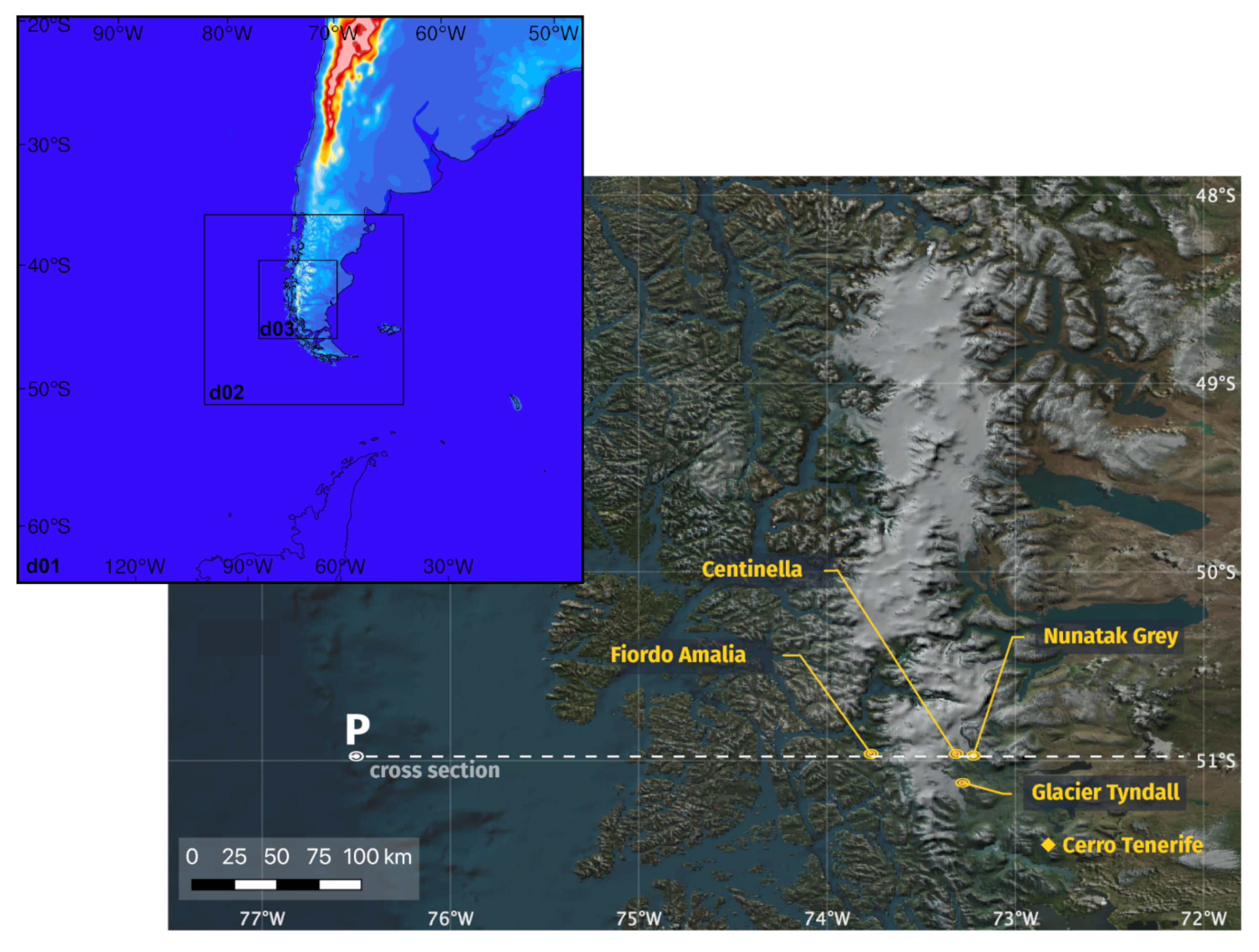
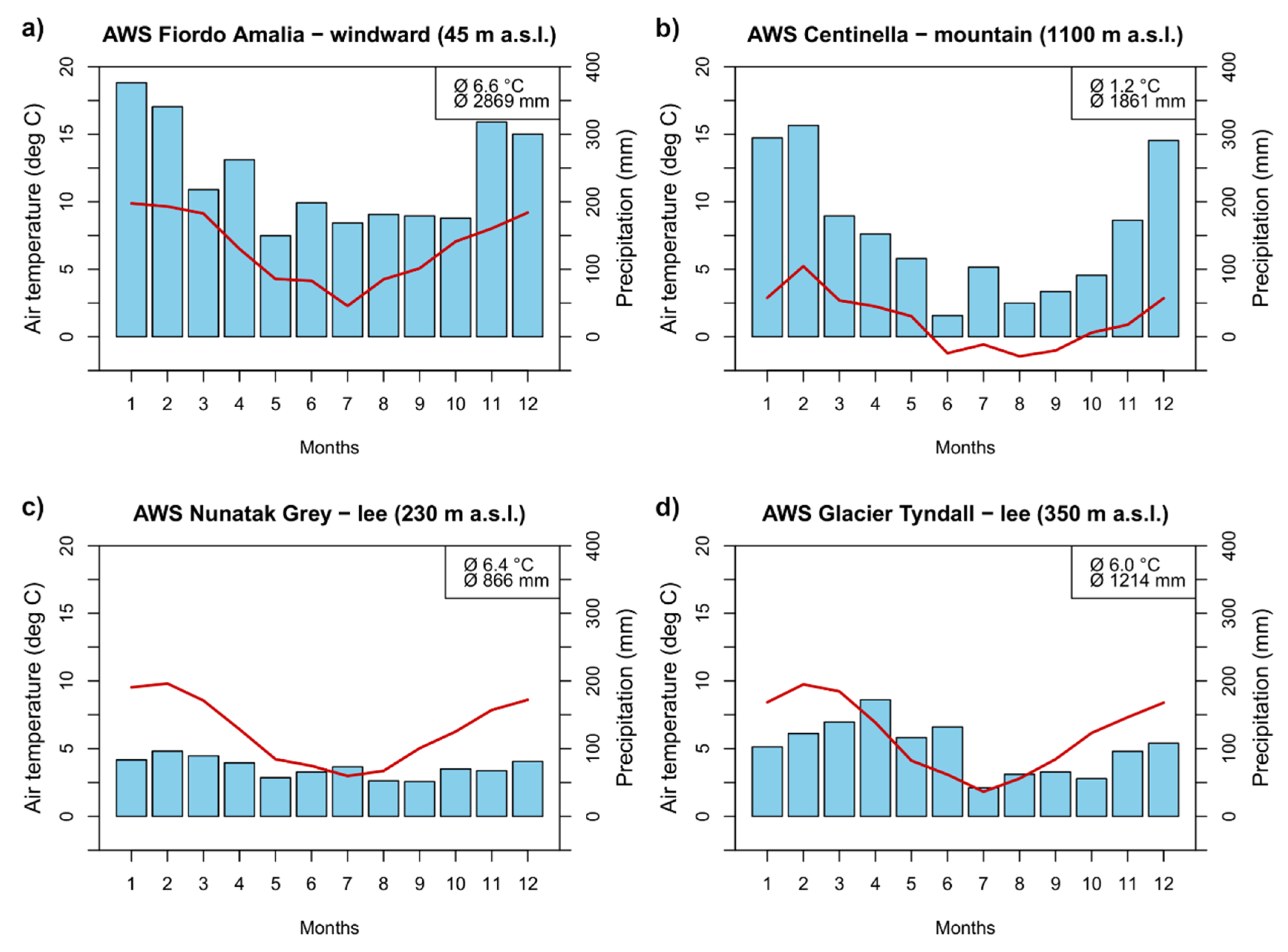
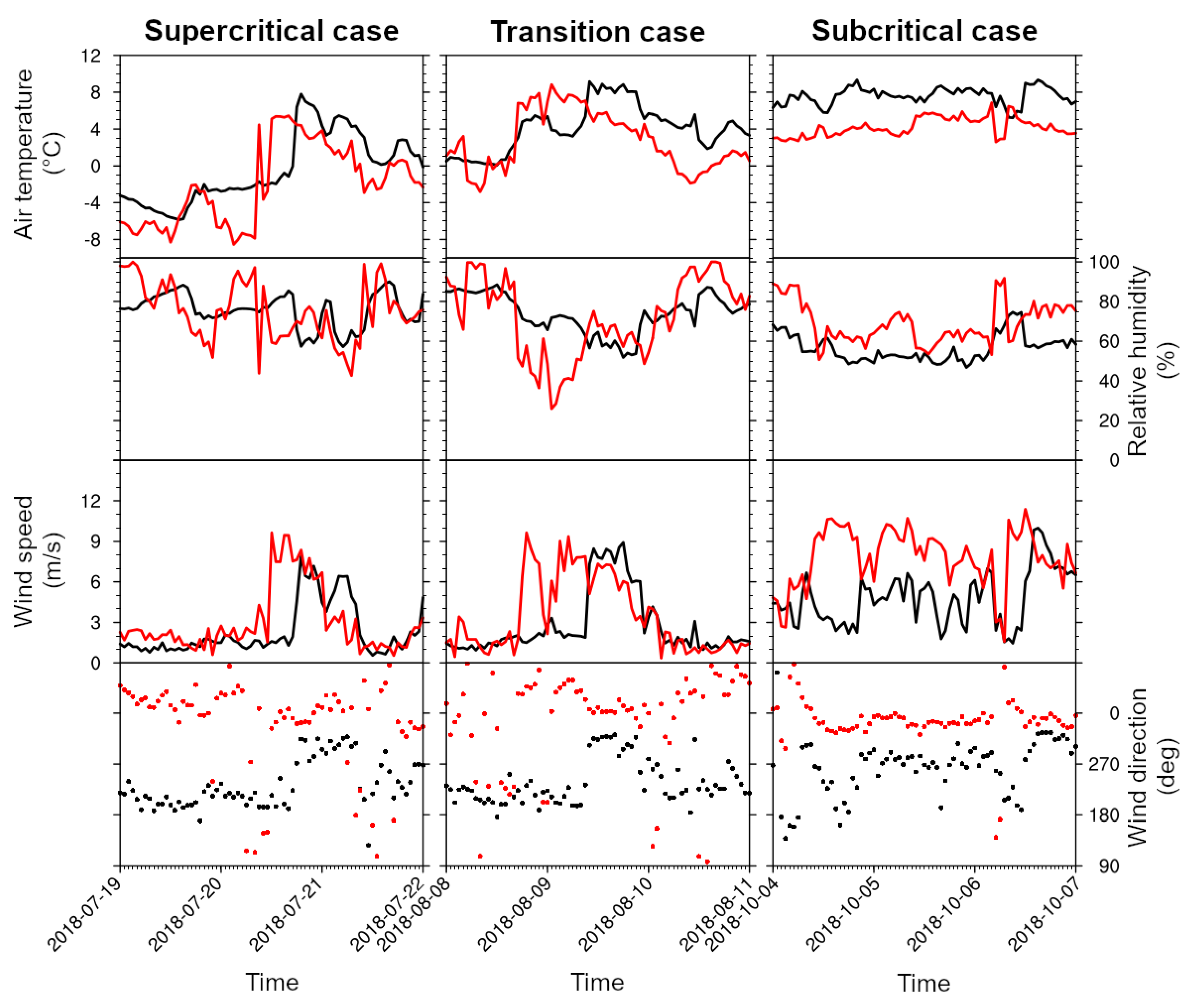
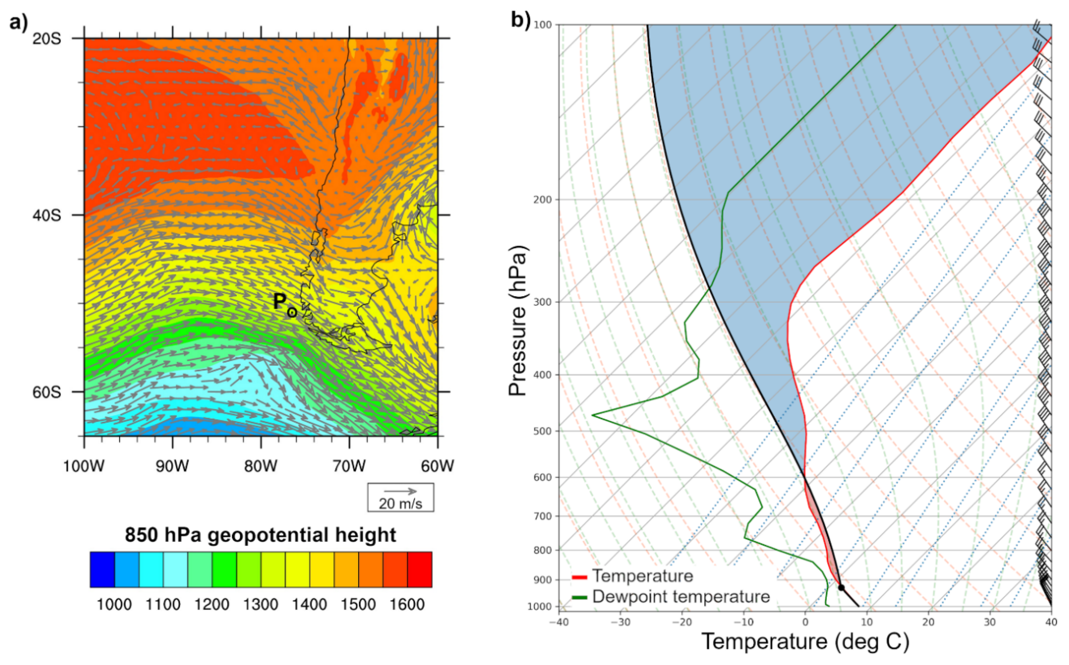
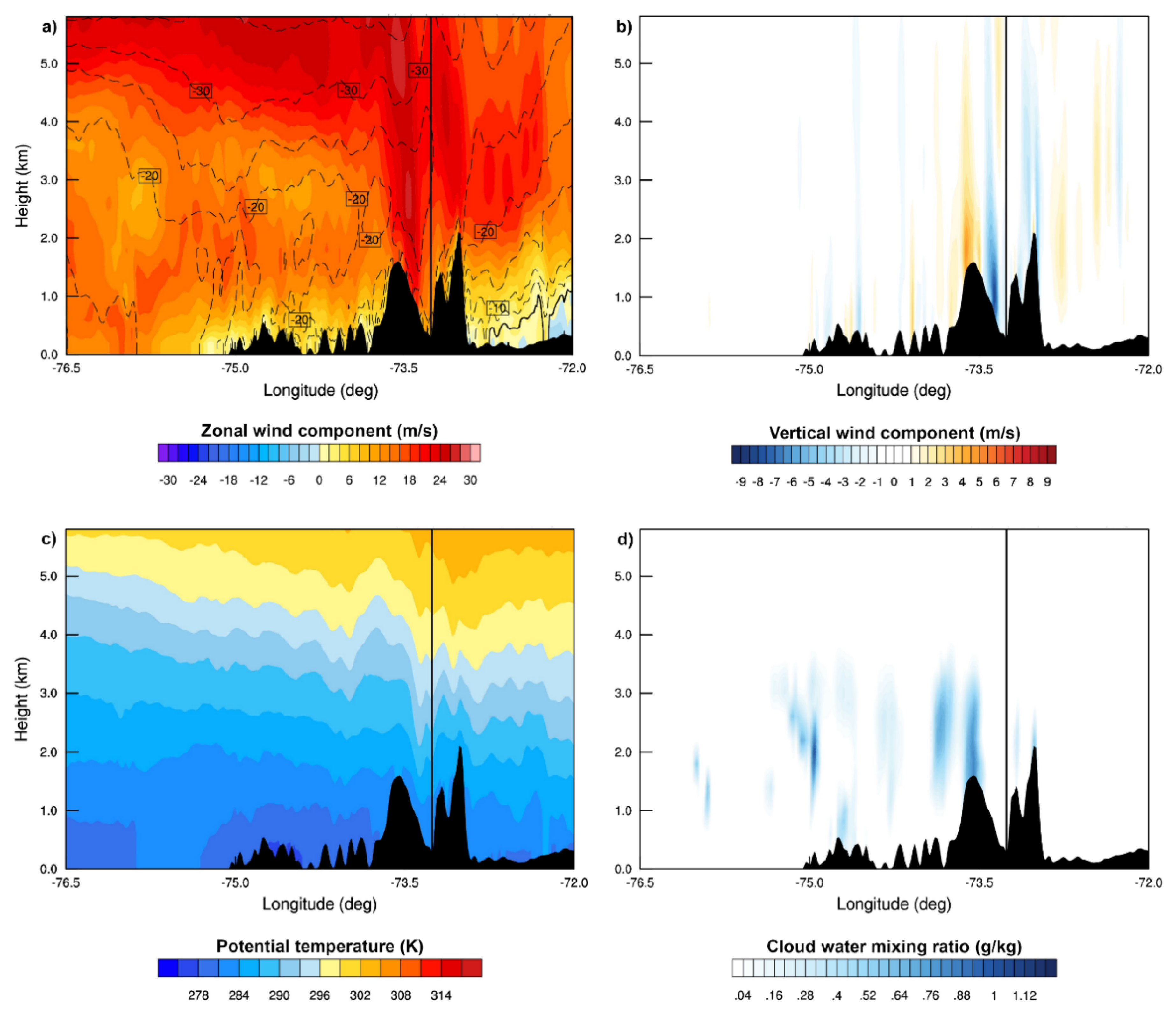
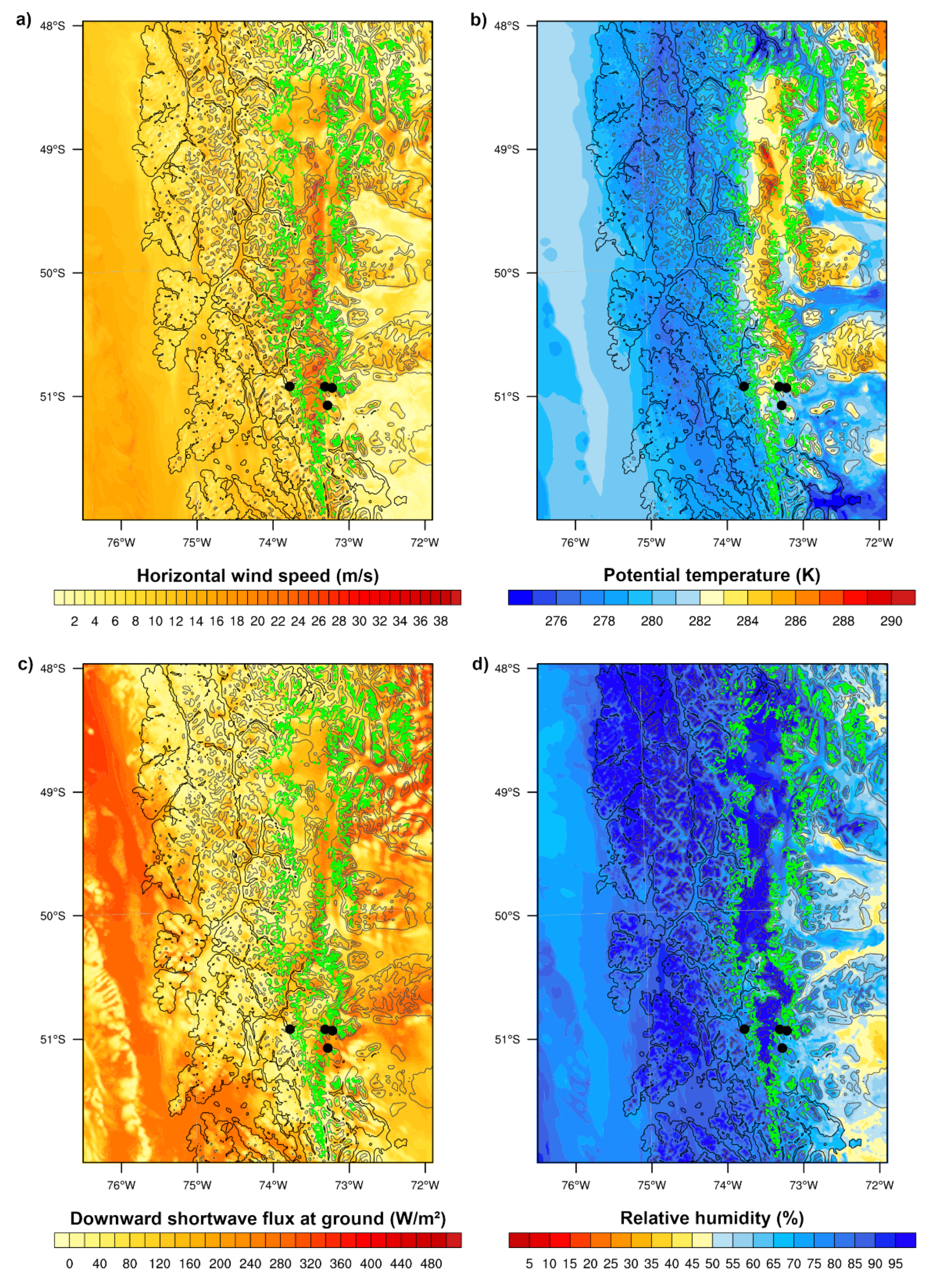
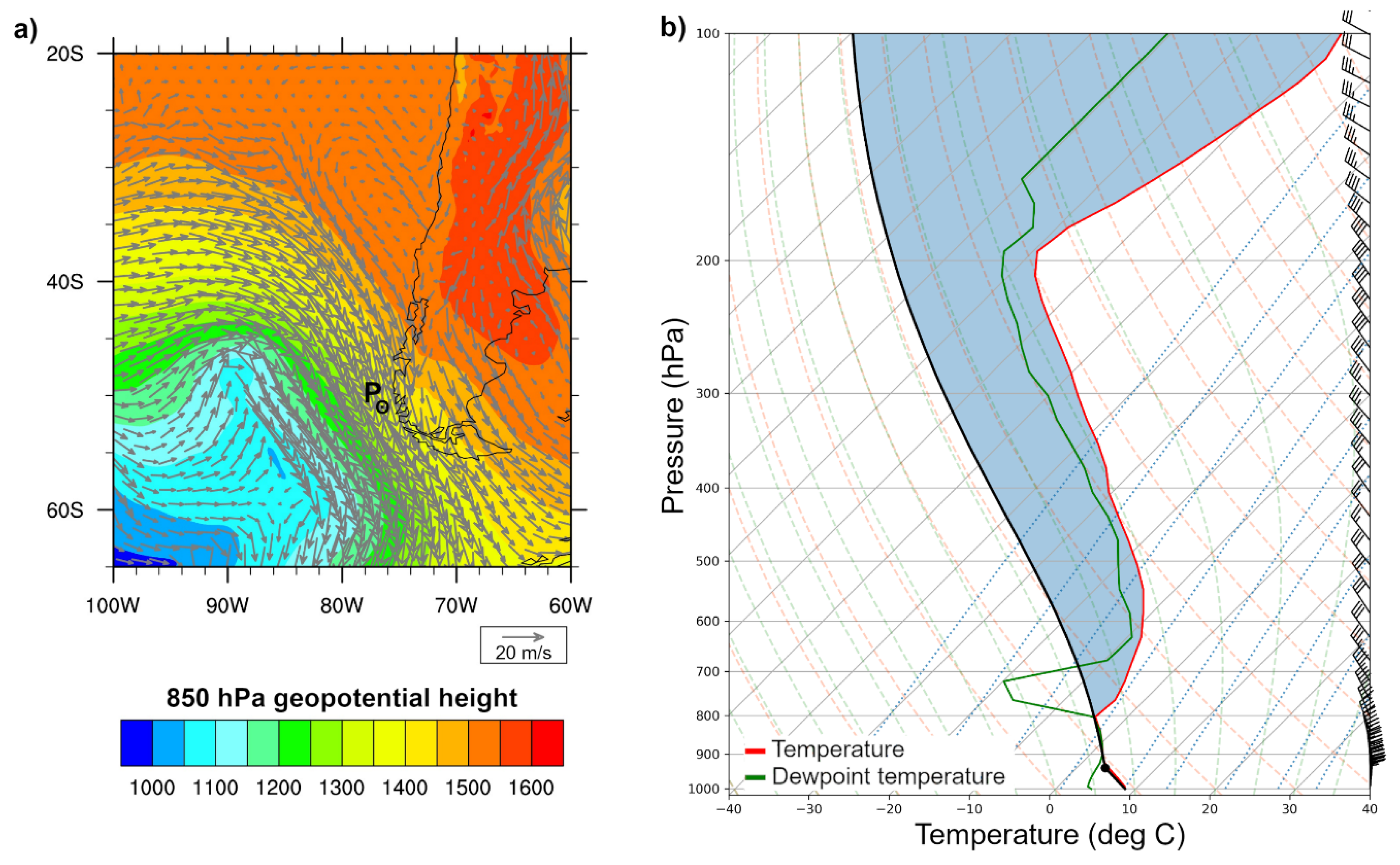
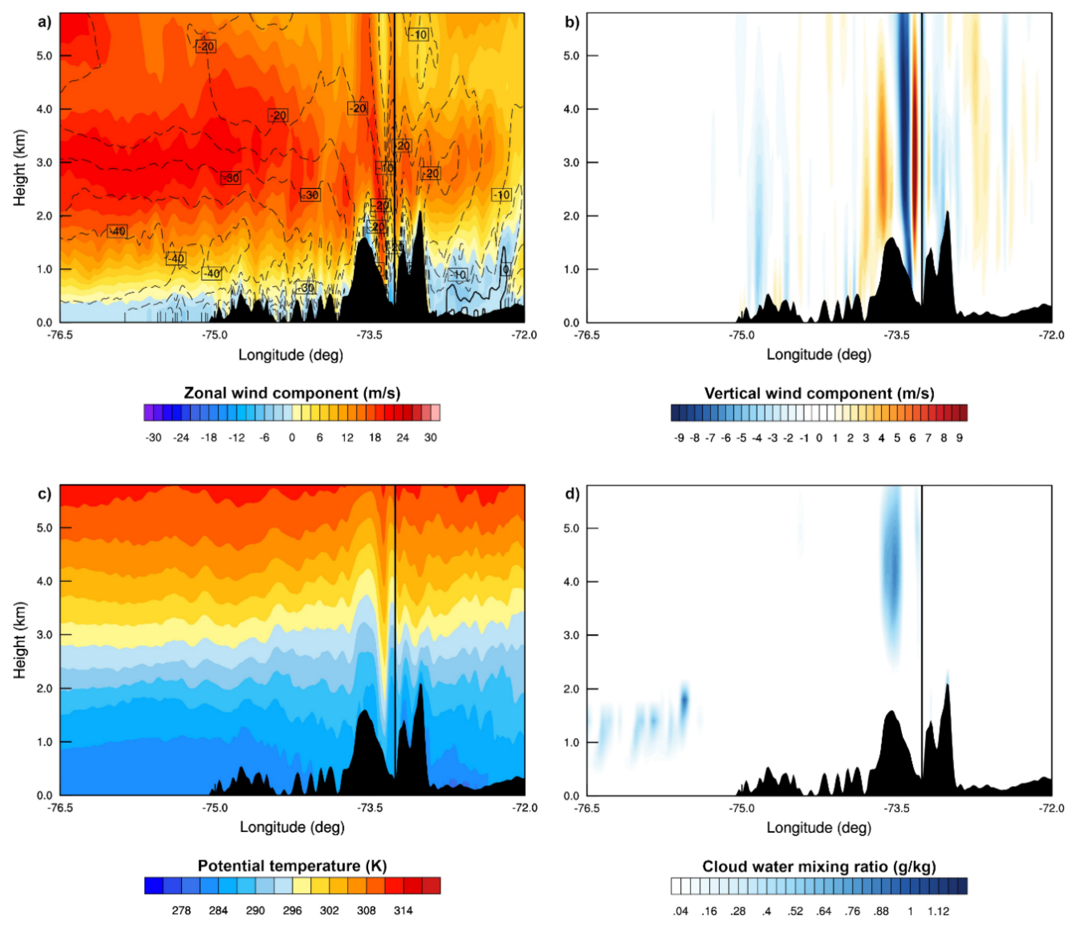
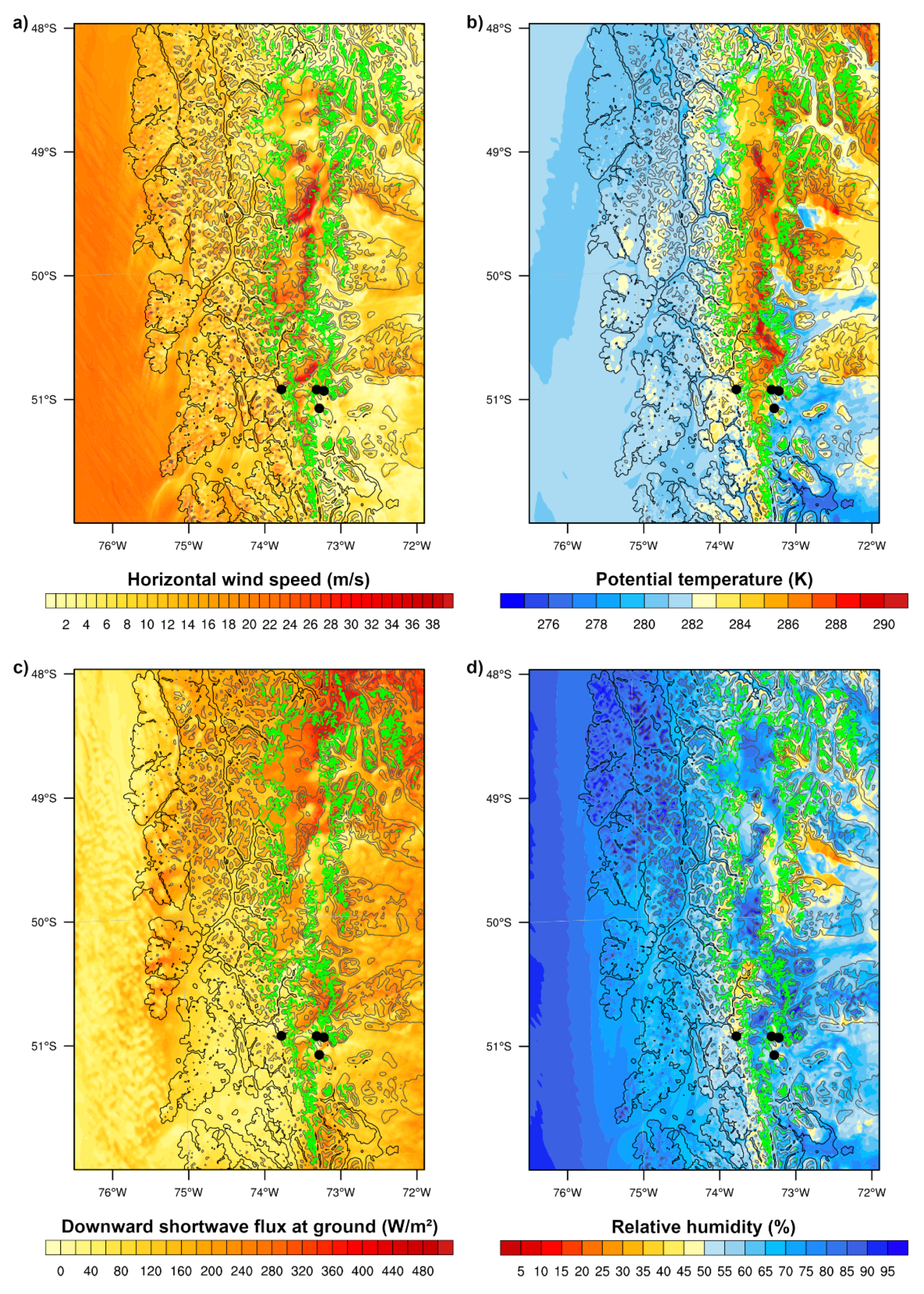
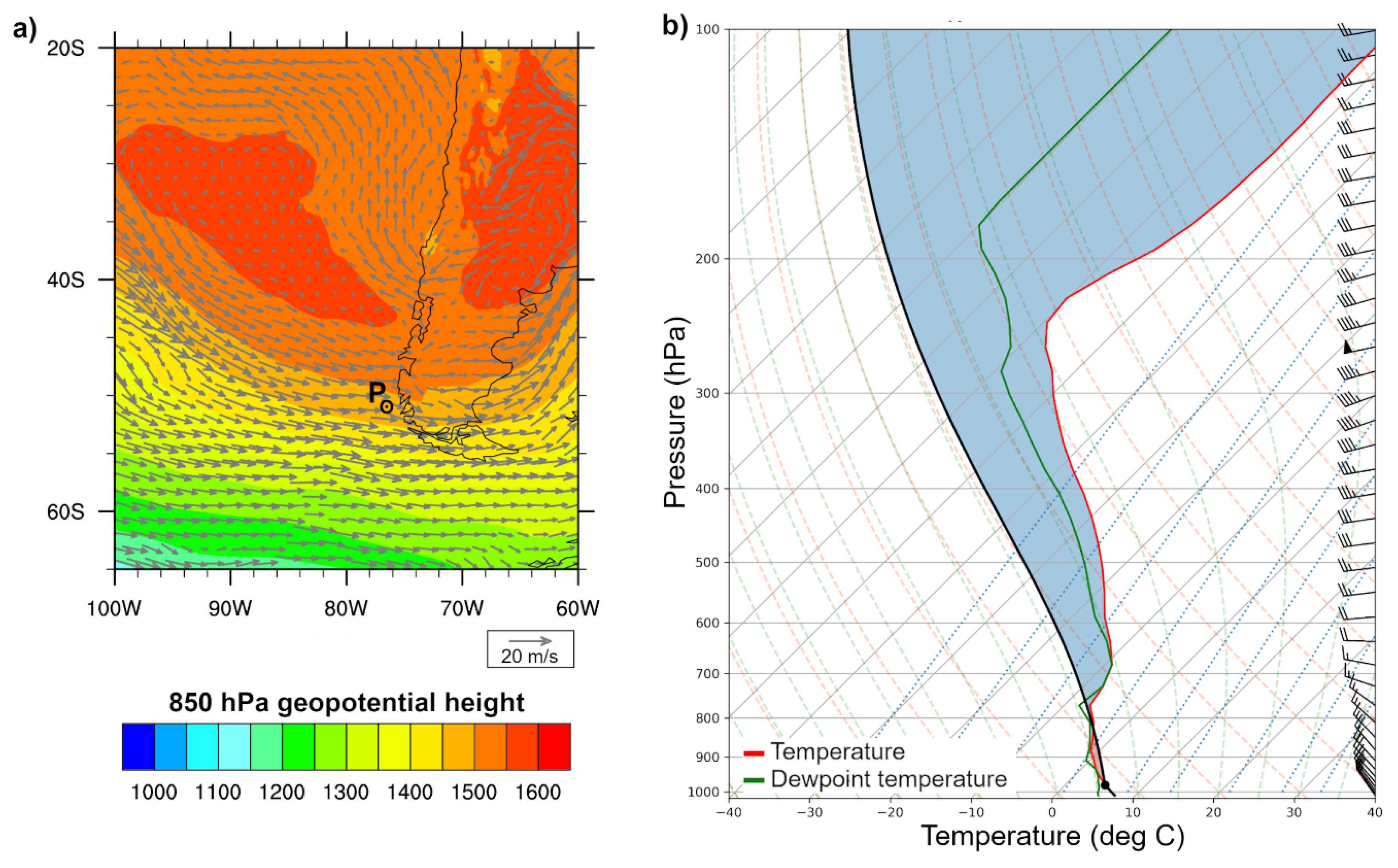
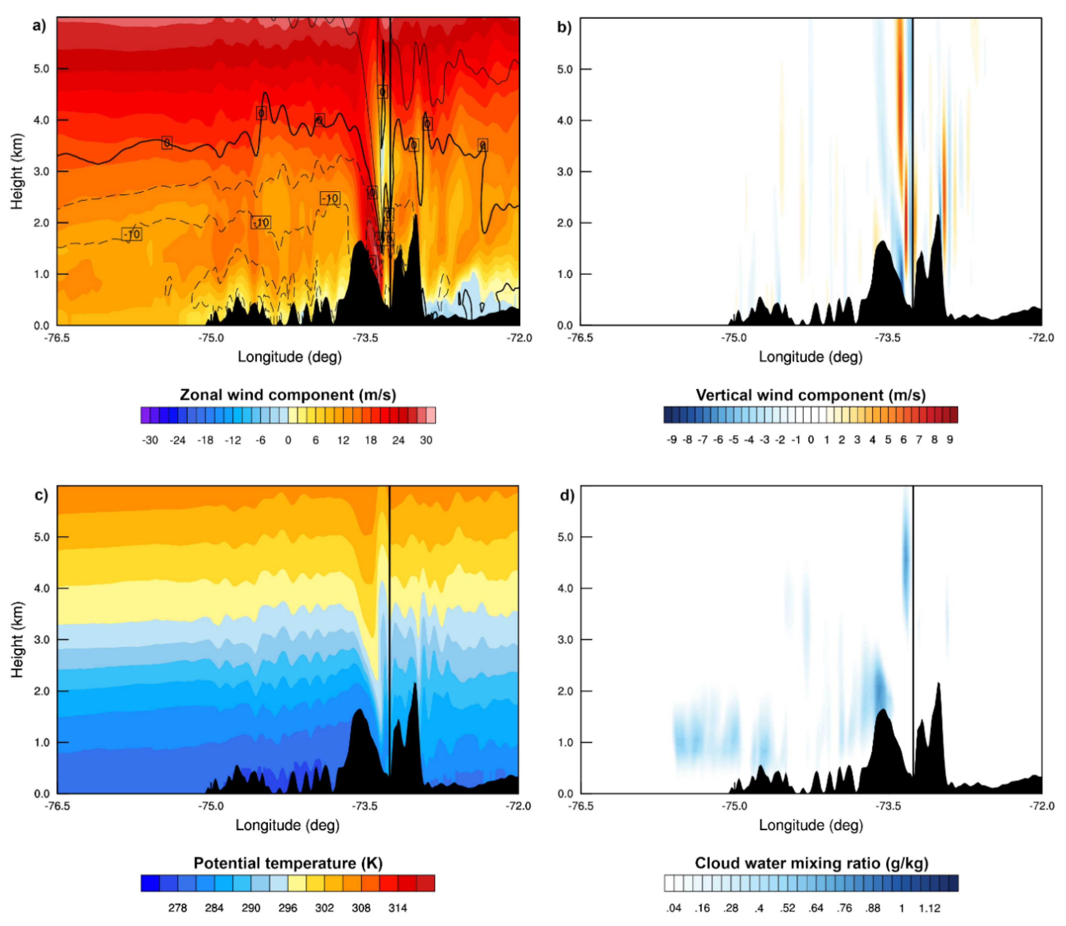
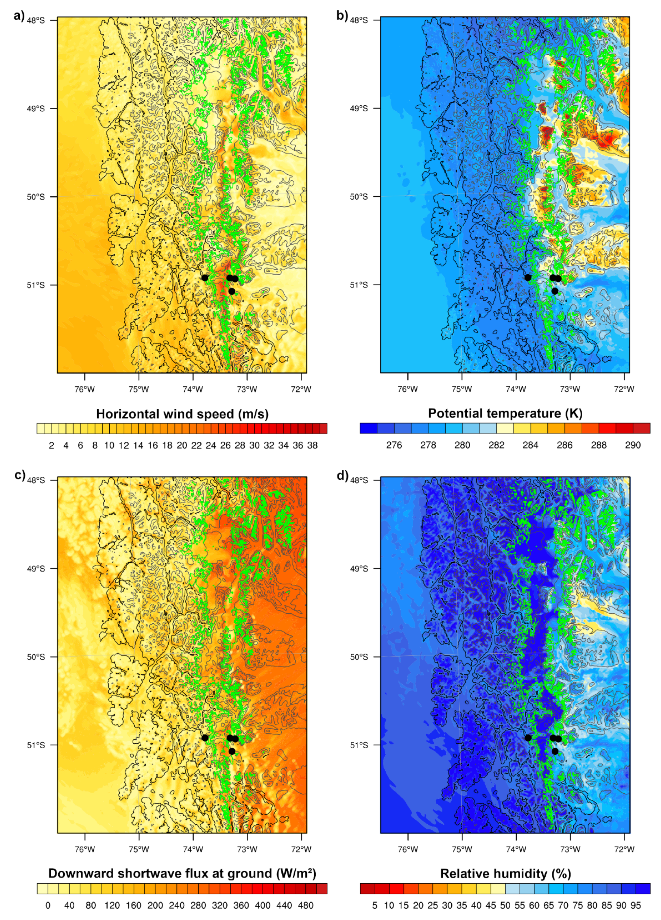
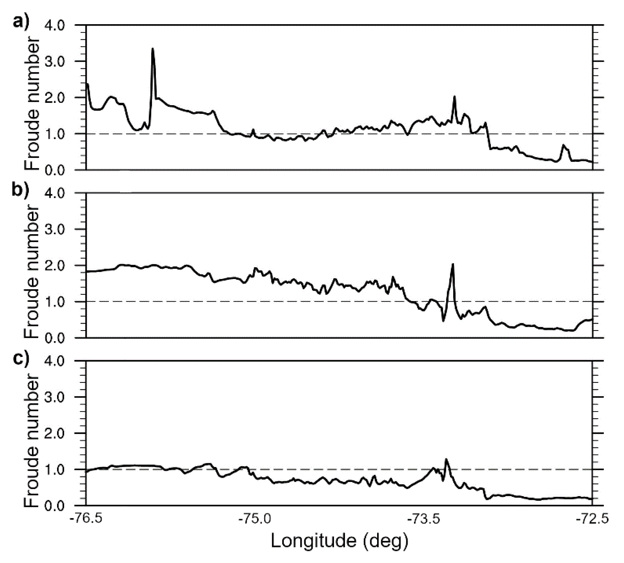
Table 1.
Automatic weather stations (AWSs) and their locations, measured variables (air temperature T, relative humidity RH, global (total incoming shortwave) radiation G, wind speed U, wind direction Dir and precipitation R) and recording times.
Table 1.
Automatic weather stations (AWSs) and their locations, measured variables (air temperature T, relative humidity RH, global (total incoming shortwave) radiation G, wind speed U, wind direction Dir and precipitation R) and recording times.
| AWS | Altitude | Location | Variables | Available Data Since | Temporal Resolution |
|---|---|---|---|---|---|
| FA (windward) | 45 m | 50°57′44.7″ S, 73°46′06.2″ W | T, RH, R | 2015 | Daily, hourly |
| CE (mountain) | 1100 m | 50°57′54.5″ S, 73°18′54.0″ W | T, RH, G, U, Dir, R | 2017 | Hourly |
| NG (lee) | 230 m | 50°58′32.0″ S, 73°13′19.0″ W | T, RH, G, U, Dir, R | 2015 | 10 min |
| GT (lee) | 350 m | 51°07′01.6″ S, 73°16′56.7″ W | T, RH, U, Dir, R | 2011 | Daily, hourly |
Table 2.
Sensor types and accuracies of AWSs Centinella (CE) and Nunatak Grey (NG).
| Variable | Sensor Name | Accuracy |
|---|---|---|
| Temperature and Humidity | Campbell Scientific CS215 | ±0.4 °C ±4.0% |
| Wind | Campbell Scientific Young 05108-45-L | ±0.3 m/s or 1% |
| Radiation | Campbell Scientific CS300 | ±5.0% of total daily radiation |
| Precipitation | Campbell Scientific Young 52202-L | ±3.0% up to 50 mm/h up to 50.0% local wind undercatch |
Table 3.
WRF model setup.
| Parameter | Selection |
|---|---|
| Topography resolution | 500 m (SRTM) |
| Land use | Land cover classification system (LCCS) |
| Horizontal resolution | d01: 20 km, d02: 4 km, d03: 1 km |
| Vertical resolution | 50 levels |
| Nesting | One-way grid nesting with default coefficients for u, v, θ and q above the planetary boundary layer |
| Nudging | 3-hourly on d01 |
| Land surface physics | Noah multi-physics land surface model |
| Microphysics | Morrison double-moment micro-physic scheme |
| Radiation (longwave and shortwave) | Rapid radiative transfer model (RRTMG) scheme |
| Surface layer physics | Mellor–Yamada–Nakanishi–Niino (MYNN) surface layer scheme |
| Planetary boundary layer | MYNN2 boundary layer scheme |
| Convection | Kain–Fritsch convection scheme (d01 and d02) |
Table 4.
Statistics of the model evaluation (mean model bias, MMB, root mean square error, RMSE, and Pearson correlation coefficient, r) at each AWS for the supercritical, transition and subcritical cases. Simulated wind speeds have been extrapolated from 10 to 2 m to be comparable with measurements. The MMB and RMSE are in the respective variable’s unit. Correlations that are not statistically significant (p-value > 0.1) are greyed out.
| AWS | Statistic | Supercritical Case | Transition Case | Subcritical Case | ||||||
|---|---|---|---|---|---|---|---|---|---|---|
| T | RH | U | T | RH | U | T | RH | U | ||
| FA | MMB | 0.55 | −12.66 | - | −0.74 | −6.64 | - | −1.75 | 5.95 | - |
| RMSE | 2.32 | 24.11 | - | 1.73 | 19.94 | - | 1.94 | 9.61 | - | |
| r | 0.72 | 0.45 | - | 0.88 | 0.55 | - | 0.65 | 0.56 | - | |
| CE | MMB | −2.08 | 1.82 | - | −1.88 | −0.13 | - | −1.20 | 12.43 | - |
| RMSE | 2.87 | 13.10 | - | 2.64 | 16.14 | - | 1.72 | 16.59 | - | |
| r | 0.69 | 0.91 | - | 0.63 | 0.22 | - | 0.66 | 0.60 | - | |
| NG | MMB | −1.66 | −1.26 | 0.87 | −1.35 | −1.79 | 0.71 | −3.40 | 12.77 | 3.02 |
| RMSE | 3.21 | 12.72 | 2.37 | 3.22 | 16.74 | 2.73 | 3.63 | 15.62 | 4.23 | |
| r | 0.78 | 0.59 | 0.68 | 0.50 | 0.56 | 0.47 | 0.13 | 0.51 | −0.02 | |
| GT | MMB | −0.41 | −6.12 | 0.59 | −0.55 | −0.85 | 0.16 | −3.10 | 21.43 | 1.69 |
| RMSE | 2.20 | 14.16 | 1.90 | 2.64 | 13.55 | 2.36 | 3.28 | 22.93 | 3.70 | |
| r | 0.83 | 0.07 | 0.48 | 0.49 | 0.43 | 0.37 | 0.73 | 0.54 | −0.04 | |
Table 5.
Anomalies of incoming shortwave radiation (SWin), turbulent latent heat flux (Hlat) and turbulent sensible heat flux (Hsen) during föhn activity for supercritical, transition and subcritical cases at two locations. Anomalies compare the average during the peak of each föhn event to the average of all simulations. Fmelt gives the fraction of all melt hours that coincide with the respective föhn event for each simulation individually.
| Variable | Supercritical Case | Transition Case | Subcritical Case | |||
|---|---|---|---|---|---|---|
| NG | CE | NG | CE | NG | CE | |
| SWin (W/m2) | +100.7 | +122.5 | +63.2 | +87.5 | +137.8 | +39.9 |
| Hlat (W/m2) | −3.3 | +0.5 | −21.5 | −131.4 | −52.3 | −48.5 |
| Hsen (W/m2) | +94.8 | −19.1 | +72.4 | +106.1 | +157.7 | +14.3 |
| Fmelt (%) | 46.6 | - | 75.7 | 100 | 39.8 | 47.4 |
© 2020 by the authors. Licensee MDPI, Basel, Switzerland. This article is an open access article distributed under the terms and conditions of the Creative Commons Attribution (CC BY) license (http://creativecommons.org/licenses/by/4.0/).
Share and Cite
MDPI and ACS Style
Temme, F.; Turton, J.V.; Mölg, T.; Sauter, T. Flow Regimes and Föhn Types Characterize the Local Climate of Southern Patagonia. Atmosphere 2020, 11, 899. https://doi.org/10.3390/atmos11090899
AMA Style
Temme F, Turton JV, Mölg T, Sauter T. Flow Regimes and Föhn Types Characterize the Local Climate of Southern Patagonia. Atmosphere. 2020; 11(9):899. https://doi.org/10.3390/atmos11090899
Chicago/Turabian StyleTemme, Franziska, Jenny V. Turton, Thomas Mölg, and Tobias Sauter. 2020. "Flow Regimes and Föhn Types Characterize the Local Climate of Southern Patagonia" Atmosphere 11, no. 9: 899. https://doi.org/10.3390/atmos11090899
Note that from the first issue of 2016, this journal uses article numbers instead of page numbers. See further details here.