Factorizations of Symmetric Macdonald Polynomials

Abstract

We prove many factorization formulas for highest weight Macdonald polynomials indexed by particular partitions called quasistaircases. Consequently, we prove a conjecture of Bernevig and Haldane stated in the context of the fractional quantum Hall effect theory.

1. Introduction

Jack polynomials have many applications in physics, especially in statistical physics and quantum physics due to their relation to the many-body problem. In particular, fractional quantum Hall (FQH) states of particles in the lowest Landau levels are described by such polynomials [1,2,3]. In that context, some properties, called clustering properties, are highly relevant. A clustering property can occur for some negative rational parameters of a Jack polynomial and means that the Jack polynomial vanishes when distinct clusters of equal variables are formed. Using tools of algebraic geometry, Berkesch-Zamaere et al. [4] proved several clustering properties including some special cases conjectured by Bervenig and Haldane [1]. Coming from theoretical physics, the study of these properties raises very interesting problems in combinatorics and representation theory of the affine Hecke algebra. More precisely, the problem is studied in the realm of Macdonald polynomials which form a $(q,t)$-deformation of the Jack polynomials related to the double affine Hecke algebra and the results are recovered by making degenerate the parameters q and t. Recently, a very similar technique has been used in [5] to prove general formulas for perturbative correlators in basic matrix models that can be interpreted as the Schur-preservation property of Gaussian measures. In this case, the substitution of Schur functions by Macdonald polynomials defines a deformation of the matrix model. For our case, instead of stating the results in terms of clustering properties, we prefer to state them in terms of factorizations. Indeed, clustering properties are shown to be equivalent to very elegant formulas involving factorizations of Macdonald polynomials. For instance, many such factorizations have already been investigated in [6,7,8,9]. In particular, this paper is the sequel of [9] in which two of the authors proved factorizations for rectangular Macdonald polynomials. In this paper, we investigate factorizations for more general partitions, called quasistaircase partitions.

The paper is organized as follows. In Section 2, we recall essential prerequisites on Macdonald polynomials. In Section 3, we give a brief account on the physics motivations coming from the FQH effect theory. In Section 4, we investigate some factorizations involved for generic values of $(q,t)$. Section 5 is devoted to the special cases of specializations of the type $t^a{q}^b=1$ and, in particular, to the consequences on spectral vectors. In Section 6, we deduce factorizations from the results of Feigen et al. [10] and, in Section 7, we prove more general results which are consequences of the highest weight (HW) condition of some Macdonald polynomials indexed by quasistaircase partitions proved in [11]. Section 8 is devoted to illustrate our results by proving a conjecture stated by Bernevig and Haldane [2] and also we show many other examples of factorizations that do not follow from our formulas.

2. Background

This paper is focused on the study of four variants of the Macdonald polynomials: symmetric, nonsymmetric, shifted symmetric and shifted nonsymmetric. Before getting into the results, we introduce these polynomials as well as some useful notation. All the results contained in this section are well known results showed in several papers (see, e.g., [12,13,14,15,16,17,18,19,20]). The results of [21,22,23] are extensively used throughout our paper.

2.1. Partitions and Vectors

A partition $\lambda =[{\lambda }_1,\dots ,{\lambda }_{\ell }]$ of n is a weakly decreasing sequence of nonnegative integers such that $\left|\lambda \right|:={\sum }_i{\lambda }_i=n$. The length of a partition $\lambda$ is the number of nonzero parts, $\ell \left(\lambda \right)=\max \{i:{\lambda }_i>0\}$. We denote by ${\lfloor \lambda \rfloor }_i$ the number of parts of $\lambda$ lower or equal to i, and by $m_{\lambda }$ the multiplicity of the maximal part in $\lambda$.

We consider a dominance order on the partitions: Let $\lambda$ and $\mu$ be partitions, we say that $\lambda {⪯}_D\mu$ if and only if, for all i, ${\lambda }_1+\cdots +{\lambda }_i\le {\mu }_1+\cdots +{\mu }_i$.

We also consider vectors, denoting by $v=\left[v\right[1],\dots ,v[N\left]\right]$ a vector of length $\ell \left(v\right)=N$ and with nonnegative entries. We denote by $\left|v\right|$ the sum of the entries of v. For each vector v, there is a unique partition, $v^{+}$, which is a permutation of v. The dominance order defined on partitions extends to vectors with the same definition. In addition, we define another order: For u and v vectors, we say that $u⪯v$ if and only if either $u^{+}{⪯}_D{v}^{+}$ or $\left(u^{+}=v^{+}\right.$ and $\left.u{⪯}_{D}v\right)$. Initially, this order is only defined for vectors such that $\left|u\right|=\left|v\right|$, and we extend it straightforwardly for any vectors by adding the condition $u\prec v$ when $\left|u\right|<\left|v\right|$.

We define the standardization of v, ${\mathrm{std}}_v$, as the vector obtained by labeling with the integers from 0 to $N-1$ the positions in v from the smallest entries to the largest one and from right to left. Moreover, we define the reciprocal vector of v as $\langle v\rangle =\left[t^{{\mathrm{std}}_v\left[1\right]}{q}^{v\left[1\right]},\dots ,t^{{\mathrm{std}}_v\left[N\right]}{q}^{v\left[N\right]}\right]$, and the reciprocal sum of v as ${\displaystyle ⟅v⟆=\sum _i\langle v\rangle \left[i\right]}$. If there is ambiguity, the indices q and t are added. Note that in the particular case of considering a partition $\lambda$, $⟅\lambda ⟆={\sum }_i{t}^{N-i}{q}^{{\lambda }_i}$.

For example, consider the vector $v=[1,2,2,0,1,1]$ of length 6. Then, $\mathrm{std}\left(v\right)=[3,5,4,0,2,1]$, $\langle v\rangle =\left[q{t}^3,q^2{t}^5,q^2{t}^4,1,q{t}^2,qt\right]$, and ${\displaystyle ⟅v⟆=1+qt+q{t}^2+q{t}^3+q^2{t}^4+q^2{t}^5}$.

2.2. Affine Hecke Algebra

We present a brief introduction to the affine Hecke algebra ${\mathcal{H}}_N(q,t)$ and the Demazure–Lusztig operators $T_i$. For more details, see [24,25,26,27].

Let $N\ge 2$ be an integer, q and t be two independent parameters, and $\mathbb{X}=\{x_1,\dots ,x_N\}$ be a set of formal variables. We consider the right operators $T_i$, for $1\le i\le N-1$, acting on Laurent polynomials in the variables $\mathbb{X}$ by

$$\begin{array}{c}\hfill T_i=t+(s_i-1)\frac{t{x}_{i+1}-x_i}{x_{i+1}-x_i},\end{array}$$

where $s_i$ is the elementary transposition permuting the variables $x_i$ and $x_{i+1}$. For instance, $1T_i=t$ and $x_{i+1}{T}_i=x_i$. In fact, the operators $T_i$ are the unique operators that commute with multiplication by symmetric functions in $x_i$ and $x_{i+1}$ satisfying these last two equations. Consider also the affine operator $\tau$ defined by

$$f(x_1,\dots ,x_N)\tau =f\left(\frac{x_N}{q},x_1,\dots ,x_{N-1}\right).$$

The operators $T_i$ satisfy the relations of the Hecke algebra of the symmetric group:

$$\begin{array}{c}\hfill T_i{T}_{i+1}{T}_i=T_{i+1}{T}_i{T}_{i+1},\mathrm{for}\mathrm{all}i,T_i{T}_j=T_j{T}_i\mathrm{for}|i-j|>1,(T_i-t)(T_i+1)=0,\mathrm{for}\mathrm{all}i.\end{array}$$

Then, together with the multiplication by variables $x_i$ and the affine operator $\tau$, they generate the affine Hecke algebra of the symmetric group:

$${\mathcal{H}}_N(q,t)=\mathbb{C}(q,t)\left[x_1^{\pm },\dots ,x_N^{\pm },T_1^{\pm },\dots ,T_{N_1}^{\pm },\tau \right].$$

2.3. Symmetric Functions and Virtual Alphabets

For the sake of simplicity, we use $\mathsf{\Lambda }$-ring notation for specializations of symmetric polynomials (see [22]). A finite alphabet is a finite set of formal variables and we denote it by $\mathbb{X}=\{x_1,x_2,\dots ,x_n\}$ or $\mathbb{X}=x_1+x_2+\cdots +x_n$. By specialization, we mean a morphism of algebras and, since we manipulate only finite alphabets, specializing an alphabet is equivalent to sending each letter to a value. Notice that this is no longer the case for infinite alphabets for which the theory is more complicated.

More precisely, we adopt the following convention stated in terms of the basis of power sums symmetric polynomials. For any variable x, alphabets $\mathbb{X}$ and $\mathbb{Y}$ and scalar $\alpha$, we set

$$\begin{array}{c}\hfill \begin{array}{c}{p}_n\left(x\right)=x^n,\\ p_n(\mathbb{X}\pm \mathbb{Y})=p_n\left(\mathbb{X}\right)\pm p_n\left(\mathbb{Y}\right),\\ p_n\left(\mathbb{X}\mathbb{Y}\right)=p_n\left(\mathbb{X}\right)p_n\left(\mathbb{Y}\right),\\ p_n\left(\alpha \mathbb{Y}\right)=\alpha ·p_n\left(\mathbb{Y}\right).\end{array}\end{array}$$

We set also the following notation: ${\mathbb{X}}_k=\{x_1,\dots ,x_k\}$ and ${\mathbb{Y}}_{a,b}=\{y_a,y_{a+1},\dots ,y_b\}$, for $a\le b$. For two alphabets $\mathbb{X}$ and $\mathbb{Y}$, the resultant of $\mathbb{X}$ and $\mathbb{Y}$ is defined as

$$\mathcal{R}(\mathbb{X};\mathbb{Y})=\prod _{(x,y)\in \mathbb{X}\times \mathbb{Y}}(x-y),$$

which is a symmetric polynomial in $\mathbb{X}$ and $\mathbb{Y}$ separately (but not in $\mathbb{X}\cup \mathbb{Y}$). Hence,

$$\begin{array}{c}\hfill \mathcal{R}(\mathbb{X}+{\mathbb{X}}^{\prime };\mathbb{Y})=\mathcal{R}(\mathbb{X};\mathbb{Y})\mathcal{R}({\mathbb{X}}^{\prime };\mathbb{Y})\mathrm{and}\mathcal{R}(\mathbb{X};\mathbb{Y}+{\mathbb{Y}}^{\prime })=\mathcal{R}(\mathbb{X};\mathbb{Y})\mathcal{R}(\mathbb{X};{\mathbb{Y}}^{\prime }).\end{array}$$

Throughout this paper, the following notation is relevant and very useful. Let $P(\mathbb{X};q,t)$ and $Q(\mathbb{X};q,t)$ be two polynomials in $\mathbb{X}$ with coefficients in q and t. We say that ${\displaystyle P(\mathbb{X};q,t)\stackrel{(\ast )}{=}Q(\mathbb{X};q,t)}$ if the equality holds up to a scalar factor consisting of powers of q and t.

2.4. Macdonald Polynomials and Variants

In this section, we set up the definitions and the notation for the different variants of Jack and Macdonald polynomials that appear in this paper. For that, we define several vectors and the basis of eigenfunctions associated. First, we define the two variants of nonsymmetric Macdonald polynomials, indexed by vectors.

Definition 1.

The $(q,t)$-version of the Cherednik operators are the operators defined by

$$\begin{array}{c}\hfill {\xi }_i:=t^{1-i}{T}_{i-1}\dots T_1\tau T_{N-1}^{-1}\dots T_i^{-1},for1\le i\le N.\end{array}$$

The nonsymmetric Macdonald polynomials ${\left\{E_v\right\}}_{v\in {\mathbb{N}}^N}$ are the unique basis of simultaneous eigenfunctions of the $(q,t)$-version of the Cherednik operators such that ${\displaystyle E_v\stackrel{(\ast )}{=}{x}^v+\sum _{u\prec v}{\alpha }_{u,v}{x}^u}$. The corresponding vector of eigenvalues is called spectral vector and its ith entry is ${\displaystyle Spec{\left(v\right)}_i=\frac{1}{{\langle v\rangle }_i}}$.

We consider also the following variant of the ${\xi }_i$ operators.

Definition 2.

The Knop–Cherednik operators are defined by

$$\begin{array}{c}\hfill {\Xi }_i:=t^{1-i}{T}_{i-1}\dots T_1\tau \left(1-\frac{1}{x_N}\right)T_{N-1}^{-1}\dots T_i^{-1}+\frac{1}{x_i},for1\le i\le N.\end{array}$$

The nonsymmetric shifted Macdonald polynomials ${\left\{M_v\right\}}_{v\in {\mathbb{N}}^N}$ are the unique basis of simultaneous eigenfunctions of the Knop–Cherednik operators such that ${\displaystyle M_v\stackrel{(\ast )}{=}{x}^v+\sum _{u\prec v}{\alpha }_{u,v}{x}^u}$.

As in the case of the nonsymmetric Macdonald polynomials, the eigenvalues make up the spectral vector $\mathrm{Spec}\left(v\right)$.

Note that the polynomial $E_v$ can be recovered as a limit from $M_v$:

$$\begin{array}{c}\hfill E_v(x_1,\dots ,x_N)=\underset{a\to 0}{\lim }{a}^{\left|v\right|}{M}_v\left(\frac{x_1}{a},\dots ,\frac{x_N}{a}\right),\end{array}$$

which follows from the relation $M_v(x_1,\dots ,x_N){=}^{(\ast )}{E}_v(x_1,\dots ,x_N)+{\sum }_{u\prec v}{\beta }_{u,v}{E}_u$.

Now, we define both variants for symmetric Macdonald polynomials, indexed by partitions, by considering the sum of the operators defined above.

The Debiard–Sekiguchi–Macdonald operator is the operator defined as $\xi ={\sum }_i{\xi }_i$. The symmetric Macdonald polynomials, $P_{\lambda }$, are defined as the eigenfunctions of $\xi$. Similarly, we can consider the operator $\Xi ={\sum }_i{\Xi }_i$ and the symmetric shifted Macdonald polynomials, $M{S}_{\lambda }$, are defined as the eigenfunctions of $\Xi$. In both cases, the eigenvalues are ${⟅\lambda ⟆}_{q^{-1},t^{-1}}$.

We define the symmetric Jack polynomials, $J_{\lambda }^{\alpha }$, as the limit of the Macdonald polynomials, $P_{\lambda }$, with $q=t^{\alpha }$ and $t\to 1$. The other versions of Jack polynomials can be also defined as a limit, but we focus our attention on the symmetric variant.

Two families of polynomials are relevant for our study and rely on the difference of the operators presented above. The differences of the Cherednik operators and the Knop–Cherednik operators are known as the Dunkl operators, $D_i={\Xi }_i-{\xi }_i$. We say that a polynomial is singular if it is in the kernel of $D_i$, for all i. We say that a polynomial is a HW polynomial if it is in the kernel of $\Xi -\xi$.

2.5. Computing Macdonald Polynomials Using the Yang–Baxter Graph

In [21], Lascoux described how to compute the nonsymmetric shifted Macdonald polynomials $M_v$ using the Yang–Baxter graph. This computation is based on the following result.

Proposition 1.

Let v be a vector.

• If $v\left[i\right]<v[i+1]$, ${\displaystyle M_{v.s_i}=M_v\left(T_i+\frac{1-t}{1-\frac{\langle v\rangle [i+1]}{\langle v\rangle \left[i\right]}}\right)}$, where $v.s_i$ is the vector obtained from v by exchanging the values $v\left[i\right]$ and $v[i+1]$.
• $M_{v\mathsf{\Phi }}=M_v\tau (x_N-1)$, where $v\mathsf{\Phi }=\left[v\left[2\right],\dots ,v\left[N\right],v\left[1\right]+1\right]$. We refer to this step as affine step.

This result provides a method to compute the polynomials $M_v$ following the Yang–Baxter graph associated to the vector v, starting with the zero vector $\left[0^N\right]$ and $M_{0^N}=1$. We illustrate how to do it for the nonsymmetric shifted Macdonald polynomials with an example. On the one side, we have the following sequence for the vectors:

$$\begin{array}{c}\hfill \left[000\right]\stackrel{\mathsf{\Phi }}{\to }\left[001\right]\stackrel{s_2=\left(23\right)}{\to }\left[010\right]\stackrel{s_1=\left(12\right)}{\to }\left[100\right]\stackrel{\mathsf{\Phi }}{\to }\left[002\right]\stackrel{s_2=\left(23\right)}{\to }\left[020\right]\stackrel{\mathsf{\Phi }}{\to }\left[201\right].\end{array}$$

Notice that we simplify the notation by writing $\left[000\right]$ for the vector $[0,0,0]$. Since our examples do not contain numbers larger than nine, there is no misunderstanding.

The sequence above corresponds to the following sequence on the polynomials:

$$\begin{array}{c}\hfill M_{\left[000\right]}\stackrel{\tau (x_3-1)}{\to }{M}_{\left[001\right]}\stackrel{T_2+\frac{1-t}{1-q{t}^2}}{\to }{M}_{\left[010\right]}\stackrel{T_1+\frac{1-t}{1-qt}}{\to }{M}_{\left[100\right]}\stackrel{\tau (x_3-1)}{\to }{M}_{\left[002\right]}\stackrel{T_2+\frac{1-t}{1-q^2{t}^2}}{\to }{M}_{\left[020\right]}\stackrel{\tau (x_3-1)}{\to }{M}_{\left[201\right]}.\end{array}$$

The nonsymmetric Macdonald polynomials are obtained following an almost similar algorithm where the affine action is substituted by $E_{v\mathsf{\Phi }}=E_v\tau x_N$. For instance, using the same sequence as before,

$$\begin{array}{c}\hfill E_{\left[000\right]}\stackrel{\tau x_3}{\to }{E}_{\left[001\right]}\stackrel{T_2+\frac{1-t}{1-q{t}^2}}{\to }{E}_{\left[010\right]}\stackrel{T_1+\frac{1-t}{1-qt}}{\to }{E}_{\left[100\right]}\stackrel{\tau x_3}{\to }{E}_{\left[002\right]}\stackrel{T_2+\frac{1-t}{1-q^2{t}^2}}{\to }{E}_{\left[020\right]}\stackrel{\tau x_3}{\to }{E}_{\left[201\right]}.\end{array}$$

The symmetric variants of the Macdonald polynomials are hence obtained by applying the symmetrizing operator $\mathcal{S}={\sum }_{\sigma \in {\mathfrak{S}}_N}{T}_{\sigma }$, where $T_{\sigma }=T_{i_1}\cdots T_{i_k}$ if $\sigma =s_{i_1}\cdots s_{i_k}$ is a shortest decomposition of $\sigma$ in elementary transpositions, to the polynomials labeled by a decreasing vector. In addition, Jack polynomials are obtained following a Yang–Baxter graph with degenerated intertwining operators.

2.6. Vanishing Properties

The shifted variants for Jack and Macdonald polynomials can be defined alternatively by interpolation. Indeed, one shows with the help of the Yang–Baxter graph that the shifted nonsymmetric Macdonald polynomials are characterized up to a global coefficient by the equations $M_v\left(\langle u\rangle \right)=0$, for any vector u satisfying $\left|u\right|\le \left|v\right|$ and $u\ne v$. That is, by specializing the variables of $\mathbb{X}$ to the entries of the vector $\langle u\rangle$ in the nonsymmetric Macdonald polynomial $M_v$.

By symmetrization, the shifted symmetric Macdonald polynomials are characterized up to a global coefficient by $M{S}_{\mu }\left(\langle \lambda \rangle \right)=0$, for any partition $\mu$ satisfying $\left|\mu \right|\le \left|\lambda \right|$ and $\mu \ne \lambda$.

In addition, vanishing properties of shifted symmetric and nonsymmetric Jack polynomials are obtained by making the equations above degenerate.

3. Clustering Properties of Jack Polynomials and the Quantum Hall Effect

3.1. A Gentle History of the Quantum Hall Effect

The quantum Hall effect is a phenomenon involving a collection of electrons restricted to move in a two-dimensional space and subject to a strong magnetic field.

The classical Hall effect was discovered by Edwin Hall in 1879 [28] and is a direct consequence of the motion of electrons in a magnetic field. More precisely, it comes from the fact that the magnetic field causes electrons to move in circles. Let us recall quickly the calculation. This phenomena is known under the name cyclotron effect and is deduced from the equations of the motion for a particle of mass m and charge $-e$ in a z-directed magnetic field of intensity B:

$$\begin{array}{c}\hfill \left\{\begin{array}{c}{\displaystyle m\frac{d^2}{d{t}^2}x=-eB\frac{d}{dt}y,}\hfill \\ {\displaystyle m\frac{d^2}{d{t}^2}y=eB\frac{d}{dt}x.}\hfill \end{array}\right.\end{array}$$

The general solution, $x\left(t\right)=x_0-rsin({\omega }_{B}t+\varphi )$ and $y\left(t\right)=y_0+rcos({\omega }_{B}t+\varphi )$, describes a circle. The parameters $x_0$, $y_0$, r and $\varphi$ are chosen arbitrary, while ${\omega }_B=\frac{eB}{m}$ is a linear function of B and is called the cyclotron frequency. Taking into account an electric field $\overrightarrow{E}$ generating the current together with a linear friction term modeled by the scattering time $\tau$, the motion equations become

$$\begin{array}{c}\hfill m\left(\frac{d}{dt}\right)\overrightarrow{v}=-e\overrightarrow{v}\wedge \overrightarrow{B}-\frac{m}{\tau }\overrightarrow{v}-e\overrightarrow{E}.\end{array}$$

This model is known under the name of Drude model [29,30] and consists in considering the electrons as classical balls. Assuming that the velocity is constant, it can be written as:

$$\begin{array}{c}\hfill \left(\begin{array}{cc}\frac{m}{2}& -eB\\ eB& \frac{m}{2}\end{array}\right)\overrightarrow{v}=\overrightarrow{E}.\end{array}$$

The current density $\overrightarrow{J}$ is related to the velocity by the equality $\overrightarrow{J}=-ne\overrightarrow{v}$, where n denotes the number of charged particles. Hence, $\overrightarrow{E}=\rho \overrightarrow{J}$ where

$$\begin{array}{c}\hfill \rho =\frac{m}{e^{2}n\tau }\left(\begin{array}{cc}1& {\omega }_B\tau \\ -{\omega }_B\tau & 1\end{array}\right)\end{array}$$

denotes the conductivity.

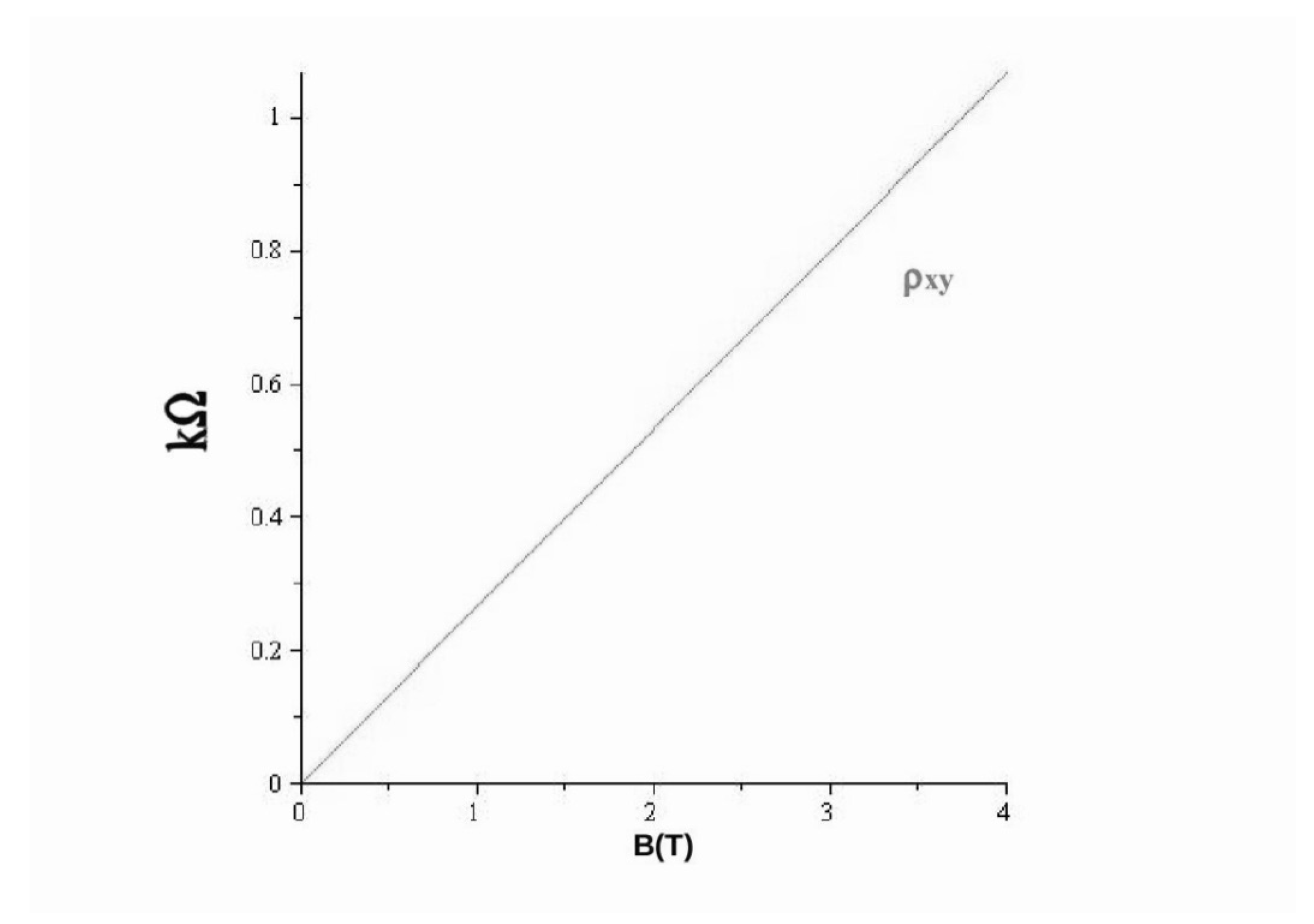
We see that there are two components to the resistivity: the off-diagonal component (Hall resistivity, see Figure 1) ${\displaystyle {\rho }_{xy}=\frac{m{\omega }_B}{e^{2}n}}$, which does not depend on $\tau$ but is linear in B, and the diagonal component (longitudinal resistivity) ${\displaystyle {\rho }_{xx}=\frac{m}{e^{2}n\tau }}$, which does not depend on B and tends to 0 when the scattering time $\tau$ tends to ∞.

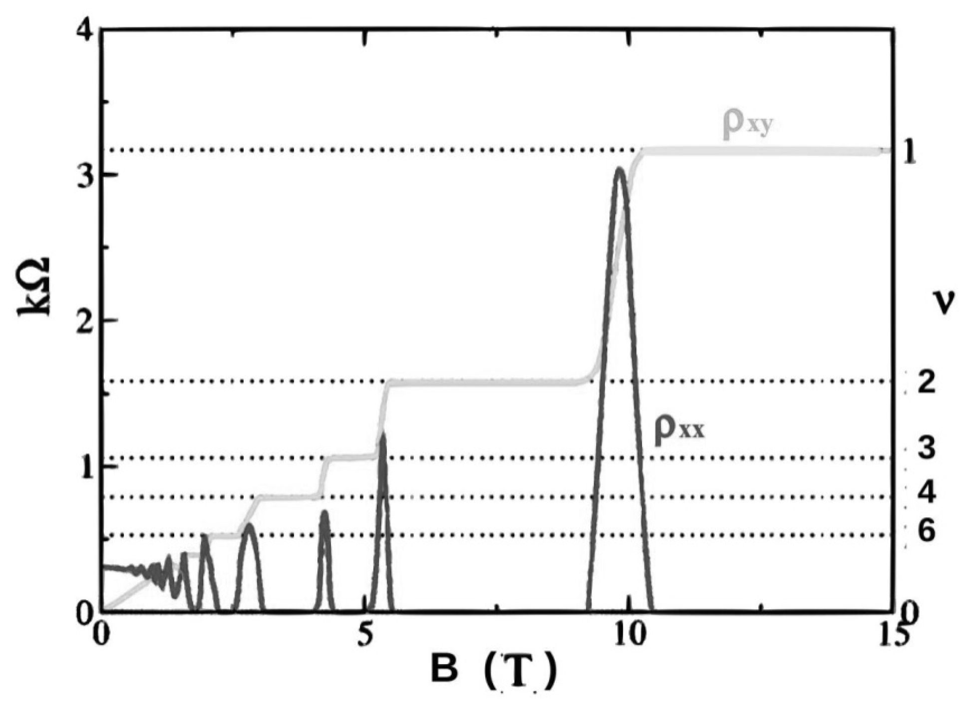
In 1980, Von Klitzing et al. [31] realized measurements of the Hall voltage of a two-dimensional electron gas with a silicon metal-oxide-semiconductor field-effect transistor and showed the Hall resistivity has fixed values. The exhibited phenomenon is called the integer quantum Hall effect, see Figure 2 (This figure was obtained by replacing the vertical scale $R_H$ by $\nu$ in [32] (Figure 4.1, Section 4.4) and it is under Creative Commons Attribution-Noncommercial-Share Alike 3.0 Generic License).

Both the Hall resistivity and longitudinal resistivity have a behavior which highlights a quantum phenomena at the mesoscopic scale. The Hall resistivity is no longer a linear function of B but sits on a plateau for a range of magnetic field before jumping to the next one. These plateaux are centered on values ${\displaystyle B_{\nu }=r_q\frac{n}{\nu }}$, where ${\displaystyle r_q=\frac{2\pi \hslash }{e}}$ is the quantum resistivity, depending on a parameter $\nu \in \mathbb{Z}$ and the Hall resistivity takes the value ${\displaystyle {\rho }_{xy}=\frac{r_q}{\nu }}$. The longitudinal resistivity vanishes when ${\rho }_{xy}$ sits on a plateau and spikes when ${\rho }_{xy}$ jumps to the next one.

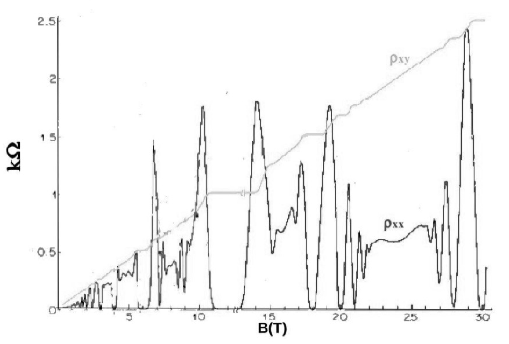
The FQH effect was discovered by Tsui et al. [33]. They observed that, as the disorder is decreased, the integer Hall plateaux become less prominent and other plateaux emerge for fractional values of $\nu$, see Figure 3 (This figure was drawn by modifying a picture from [34]).

The difference between the integer quantum Hall effect and the FQH effect is that, to explain the second, physicists need to take into account the interactions between the particles. The interaction between the electrons make the problem interesting from a mathematical point of view. The theoretical approach was pioneered by Laughlin [35] for $\nu =\frac{1}{2m+1}$. Since the Hamiltonian is very difficult to diagonalize, he proposed directly a wave function fulfilling several properties motivated by physical insight. The Laughlin wave function overlaps more than $99\%$ with the true ground state. From the observations of Tsui et al. and the work of Laughlin, more than 80 plateaux have been observed for various filling fractions. The description of the wave functions is one of the challenges of the study. It is in this context that Jack polynomials appear.

3.2. Quantum Hall Wave Functions

The FQH effect appears in many configurations of the gas. Indeed, the Hall voltage can be generated by the motion of the particles but also by quasi-particles or quasi-holes. Quasi-particles and quasi-holes are virtual particles that occur when matter behaves as if it contains different weakly interacting particles. The charges of these virtual particles are fractions of the electron charge and their masses are also different. However, in all cases, for fermion gases, the wave function must take the form

$$\begin{array}{c}\hfill \mathsf{\Phi }(z_1,\dots ,z_N)=\varphi (z_1,\cdots ,z_N)\prod _{i<j}(z_i-z_j)exp\left\{-\sum _{i=1}^N\frac{-|z_i{|}^2}{4{\ell }_B^2}\right\},\end{array}$$

where $\varphi$ is a symmetric polynomial, and ${\ell }_B=\sqrt{\frac{\hslash }{eB}}$ is the magnetic length, which is a characteristic length scale governing quantum phenomena in a magnetic field (see, e.g., [36] for details). This expression is obtained assuming that the system is in the lowest Landau level, where the single particle wave functions take the form $\varphi \left(z\right)=z^m{e}^{\frac{-{\left|z\right|}^2}{4{\ell }_B^2}}$, and that all the particles play the same role. This last condition is a quite puzzling point. Indeed, since the particles are placed in a finite portion of the plane, they cannot play the same role because the interactions must take into account the distance between the particles and the sides of the sample. Hence, the symmetry comes from an approximation when assuming that the number of particles tends to infinity. The Haldane approach [37] for this theory consists in placing the particles on a sphere. The position of a particle is specified by spinor coordinates $u=cos\left(\frac{1}{2}\theta \right)e^{i\frac{1}{2}\psi }$ and $v=sin\left(\frac{1}{2}\theta \right)e^{i\frac{1}{2}\psi }$. When the radius tends to infinity the two approaches coincide and the wave functions in the spherical geometry are used to compute approximation for the plane geometry via stereographic projection. All operators and wave function introduced by Haldane have been translated by this way in the plane geometry. In the following, we consider the Haldane point of view after stereographic projection.

The Laughlin wave function [35] models the simplest FQH states which occurs for $\nu =\frac{1}{m}$. This wave function is given by

$$\begin{array}{c}\hfill {\varphi }_{Laughlin}^m(z_1,\dots ,z_N):=\prod _{i<j}{(z_i-z_j)}^{2m}.\end{array}$$

Notice that ${\varphi }_{Laughlin}$ can be seen as the stereographic projection of Haldane wave function stated in terms of spinor coordinates by

$$\begin{array}{c}\hfill {\varphi }_{Haldane}^m=\prod _{i<j}{(u_i{v}_j-u_j{v}_i)}^{2m}.\end{array}$$

In the Laughlin states no quasi-particle or quasi-hole is involved. From a mathematical point of view, the absence of quasi-particle and quasi-hole is interpreted in terms of differential operators as follows: We consider the operators $E_n:={\sum }_i{z}_i^n\frac{\partial }{\partial z_i}$ and we set $L^{+}=E_0$ and $L^{-}=N_{\varphi }{\sum }_i{z}_i-E_2$ where $N_{\varphi }=2\frac{\mathrm{deg}\varphi }{N}$. The parameter $N_{\varphi }$ is interpreted in the spherical geometry by the fact that the sphere surrounds a monopole with charge $N_{\varphi }$. The absence of quasi-particle is characterized by $L^{+}\varphi =0$ (HW condition) while the absence of quasi-hole is characterized by $L^{-}\varphi =0$ (lowest weight (LW) condition). Noticing that $[E_m,E_n]=(m-n)E_{n+m-1}$, we find that if P is a polynomial satisfying the HW and LW conditions then $E_{1}P=\frac{1}{2}[E_2,E_0]P=-\frac{1}{2}{E}_0{E}_{2}P=\frac{1}{2}{N}_{\varphi }NP=\mathrm{deg}\left(P\right)P$, that is P is an homogeneous polynomial. The HW condition means that the polynomial is invariant by translations. A fast computation shows that ${\varphi }_{Laughlin}$ is both a HW and a LW state.

Other interesting wave functions have been exhibited. For instance, the Moore–Read (Pfaffian) state [38] is

$$\begin{array}{c}\hfill {\varphi }_{MR}^0=\prod _{i<j}(z_i-z_j)\mathrm{Pf}\left(\frac{1}{z_i-z_j}\right),\end{array}$$

where $\mathrm{Pf}$ denotes the Pfaffian. Surprisingly, it describes the FQH for $\nu =1$. To understand the difference with the integer quantum Hall effect, physicists introduced two values k and r such that $\nu =\frac{k}{r}$. The parameter k means that the function vanishes for $k+1$ particles together but not for k and the parameter r is the order of the zeros. For instance, in the Laughlin state, we have $r=2m$ and $k=1$, while for the Moore–Read state we have $r=2$ and $k=2$. In [1,2], Bernevig and Haldane showed how to associate to each Hall state an occupation number configuration. The occupation number configuration is a vector ${\mathbf{n}}_{\varphi }$ such that ${\mathbf{n}}_{\varphi }\left[i\right]$ is the number of particles in the ith lowest Landau level orbital ($i\ge 0$). For a Laughlin state ${\varphi }_{Laughlin}^m$, we have ${\mathbf{n}}_{{\varphi }_{Laughlin}^m}=[1,0^{2m-1},1,0^{2m-1},\dots ]$. For the Moore–Read state, we have ${\mathbf{n}}_{{\varphi }_{MR}^0}=[2,0,2,0,2,\dots ]$. The number $N_{\varphi }$ is the greatest integer i such that $n_{\varphi }\left[i\right]\ne 0$. Instead of using the occupation number configuration, we use a decreasing partition ${\lambda }_{\varphi }$ such that the multiplicity of the part i in ${\lambda }_{\varphi }$ equals ${\mathbf{n}}_{\varphi }\left[i\right]$. For instance ${\lambda }_{{\varphi }_{Laughlin}^m}=[(N-1)m,\dots ,m,0]$ and ${\lambda }_{{\varphi }_{MR}^0}=\left[2(\frac{N}{2}-1),2(\frac{N}{2}-1),\dots ,4,4,2,2,0,0\right]$ (N needs to be even for Moore–Read states). We see that $N_{\varphi }$ is the biggest part in ${\lambda }_{\varphi }$.

Reader interested by FQH effect theory can refer to [36] for a complete picture on the topic.

3.3. FQHT and Jack Polynomials

Some of the trial wave functions proposed to describe the FQHE are Jack functions. This is the case of the simplest one,

$$\begin{array}{c}\hfill {\displaystyle {\varphi }_{Laughlin}^m(z_1,\dots ,z_N)\stackrel{(\ast )}{=}{J}_{\left[2\right(N-1)m,2(N-2)m,\dots ,0]}^{\left(\frac{-2}{2m-1}\right)}(z_1,\dots ,z_N).}\end{array}$$

This was first noticed by Bernevig and Haldane [1]. They obtained this equality by proving that ${\varphi }_{Laughlin}^m$ is an eigenstate of the Laplace–Beltrami operator

$$\begin{array}{c}\hfill {\mathcal{H}}^{\left(\alpha \right)}=\sum _i{\left(z_i\frac{\partial }{\partial z_i}\right)}^2+\frac{1}{\alpha }\sum _{i<j}\frac{z_i+z_j}{z_i-z_j}\left(z_i\frac{\partial }{\partial z_j}-z_j\frac{\partial }{\partial z_i}\right).\end{array}$$

It is particularly interesting to remark that the main argument of the proof comes from clustering properties. Indeed, the idea is that the Laughlin wave function, considered as a polynomial in $z_i$ for some $i\in \{1,\dots ,N\}$, has a multiplicity $2m$ root at $z_i=z_j$ for any $j\ne i$. Therefore, it vanishes under the action of the operator $D_i^{L,2m}$ where $D_i^{L,r}=\frac{\partial }{\partial z_i}-r{\sum }_{j\ne i}\frac{1}{z_i-z_j}$. Since ${\varphi }_{Lauglin}^m$ is in the kernel of ${\sum }_i{z}_i{D}_i^{L,1}{z}_i{D}_i^{L,r}={\mathcal{H}}^{\left(-\frac{2}{2m-1}\right)}-\frac{m}{6}N(N-1)(N+1+6m(N-1))$, it is an eigenfunction of ${\mathcal{H}}^{\left(-\frac{2}{2m-1}\right)}$. Hence, ${\varphi }_{Laughlin}^m$ is identified with $J_{\left[2\right(N-1)m,2(N-2)m,\dots ,0]}^{\left(\frac{-2}{2m-1}\right)}(z_1,\dots ,z_N)$ by considering its dominant monomial.

In the same paper [1], a similar (but a little more complicated) reasoning is used to study the Moore–Read state ${\varphi }_{MR}^0$ described in [38]. They proved that

$$\begin{array}{c}\hfill {\displaystyle {\varphi }_{MR}^0(z_1,\dots ,z_N)\stackrel{(\ast )}{=}{J}_{\left[2(\frac{N}{2}-1),2(\frac{N}{2}-1),\dots ,4,4,2,2,0,0\right]}^{(-3)}(z_1,\dots ,z_N).}\end{array}$$

Other examples are treated in [1]. For instance, a generalization of the previous example is given by the $Z_p$ parafermionic states

$$\begin{array}{c}\hfill {\displaystyle {\varphi }_{RR}^0=\mathcal{S}\left(\prod _{k=1}^N\prod _{(k-1)N^{\prime }\le i<j\le k{N}^{\prime }}{(z_i-z_j)}^2\right)\stackrel{(\ast )}{=}{J}_{[{\left(2(N^{\prime }-1)\right)}^p,\dots ,2^p,0^p]}^{-(p+1)}(z_1,\dots ,z_N),}\end{array}$$

where $N=p{N}^{\prime }$ and $\mathcal{S}$ denotes the symmetrizing operator. This example is a special case of a Read–Rezayi state for $\nu =\frac{p}{2}$ [39]. A more complicated example is involved at $\nu =\frac{2}{5}$ and refereed to as “Gaffnian” [40]. This wave function is also proved to be a Jack polynomial [1]

$$\begin{array}{c}\hfill {\displaystyle {\varphi }_G(z_1,\dots ,z_N)\stackrel{(\ast )}{=}{J}_{[3(N^{\prime }-1),3(N^{\prime }-1),3(N^{\prime }-2),3(N^{\prime }-2),\dots ,3,3,0,0}^{\left(\frac{-3}{4}\right)}(z_1,\dots ,z_N),}\end{array}$$

with $N=2N^{\prime }$.

In the aim to provide tools for the understanding of FQH states, Bernevig and Haldane investigated clustering properties of Jack polynomials, [2]. In particular, they exhibited a family of HW Jack polynomials in N variables that vanish when s distinct clusters of $k+1$ particles are formed. The corresponding partitions are ${\lambda }_{k,r,s}^{\beta }=[{(\beta r+s(r-1)+1)}^k,\dots ,{(s(r-1)+1)}^k,0^{n_0}]$ with $n_0=(k+1)s-1$ and $N=\beta k+n_0$. Notice that, in this case, the flux (i.e., the maximal degree in each variable) equals

$$\begin{array}{c}\hfill N_{\varphi }=\beta r+s(r-1)+1=\frac{r}{k}(N-k-(k+1)(s-1))+(r-1)(s-1).\end{array}$$

Bernevig and Haldane investigated three kinds of clustering properties that occur when $k+1$ and $s-1$ are coprime:

• First clustering property:$s-1$ clusters of $k+1$ particles and one cluster of k particles, with the remaining particles free.
  This situation is formalized by setting $Z_1=z_1=\cdots =z_{k+1}$, $Z_2=z_{k+1}=\cdots =z_{2(k+1)}$,⋯,$Z_{s-1}=z_{(s-2)(k+1)+1}=\cdots =z_{(s-1)(k+1)}$, and $Z_F=z_{(s-1)(k+1)}=\cdots =z_{s(k+1)-1}$. Then, the Jack polynomial $J_{{\lambda }_{k,r,s}^{\beta }}^{-\frac{k+1}{r-1}}((k+1)(Z_1+\cdots +Z_{s-1})+k{Z}_F+z_{s(k+1)}+\cdots +z_N)$ behaves as ${\displaystyle \prod _{i=s(k+1)}^N{\left(Z_F-z_i\right)}^r}$ when each $z_i$, with $i=s(k+1),\dots ,N$, tends to $Z_F$. For instance, we have

  $$\begin{array}{c}{J}_{53}^{(-2)}(2Z_1+Z_F+z_3+z_4)={\left({\mathit{Z}}_{\mathit{F}}-{\mathit{z}}_{\mathit{4}}\right)}^2{\left({\mathit{Z}}_{\mathit{F}}-{\mathit{z}}_{\mathit{3}}\right)}^{2}P(Z_1,Z_F,z_3,z_4),\mathrm{with}\hfill \\ \hfill P(Z_1,Z_F,z_3,z_4)=144{\left({\mathit{z}}_{\mathit{3}}-{\mathit{z}}_{\mathit{4}}\right)}^2\left({\mathit{z}}_{\mathit{3}}{\mathit{z}}_{\mathit{4}}+{\mathit{Z}}_{\mathit{F}}{\mathit{z}}_{\mathit{4}}+{\mathit{Z}}_{\mathit{F}}{\mathit{z}}_{\mathit{3}}-2{\mathit{Z}}_{\mathit{1}}{\mathit{z}}_{\mathit{4}}-2{\mathit{Z}}_{\mathit{1}}{\mathit{z}}_{\mathit{3}}-2{\mathit{Z}}_{\mathit{1}}{\mathit{Z}}_{\mathit{F}}+3{{\mathit{Z}}_{\mathit{1}}}^2\right).\end{array}$$
• Second clustering property: A cluster of $n_0=(k+1)s-1$ particles.
  To formalize this situation, we set $z_1=\cdots =z_{(k+1)s-1}=Z$. Then, the Jack polynomial $J_{{\lambda }_{k,r,s}}^{\left(-\frac{k+1}{r-1}\right)}(n_{0}Z+z_{n_0+1}+\dots +z_N)$ behaves as ${\displaystyle \prod _{i=s(k+1)}^N{(Z-z_i)}^{(r-1)s+1}}$, when each $z_i$ tends to Z. More specifically, for HW Jack polynomials,

  $$\begin{array}{c}\hfill {\displaystyle J_{{\lambda }_{k,r,s}^{\beta }}^{\left(-\frac{k+1}{r-1}\right)}(n_{0}Z+z_{n_0+1}+\cdots +z_N)\stackrel{(\ast )}{=}\prod _{i=s(k+1)}^N{(Z-z_i)}^{(r-1)s+1}{J}_{{\lambda }_{k,r,1}^{\beta -1}}^{\left(-\frac{k+1}{r-1}\right)}(z_{n_0+1}+\cdots +z_N).}\end{array}$$

  (1)
  For instance,

  $$\begin{array}{c}\hfill J_{53}^{(-2)}(3Z+z_4+z_5)=-144{(Z-z_4)}^3{(Z-z_5)}^3{J}_2^{(-2)}(z_4+z_5).\end{array}$$
• Third clustering property:$s-1$ clusters of $2k+1$ particles.
  By setting $s-1$ sets of variables as follows: $Z_1=z_1=\cdots =z_{2k+1}$,…, $Z_{s-1}=z_{(s-2)(2k+1)+1}=\cdots =z_{(s-1)(2k+1)}$, the HW Jack $J_{{\lambda }_{k,r,s}^{\beta }}$ satisfies

  $$\begin{array}{c}{\displaystyle J_{{\lambda }_{k,r,s}^{\beta }}^{\left(-\frac{k+1}{r-1}\right)}((2k+1)(Z_1+\dots +Z_{s-1})+z_{(s-1)(2k+1)+1}+\cdots +z_N)\stackrel{(\ast )}{=}}\hfill \\ \hfill {\displaystyle \prod _{1\le i<j\le s-1}{(Z_i-Z_j)}^{k(3r-2)}\prod _{i=1}^{s-1}\prod _{\ell =(s-1)(2k+1)+1}^N{(Z_i-z_{\ell })}^{2r-1}·J_{{\lambda }_{k,r}^{\beta -s+1}}(z_{(s-1)(2k+1)+1}+\cdots +z_N).}\end{array}$$
  For instance,

  $$\begin{array}{c}\hfill J_{64}^{\left(-2\right)}(3(Z_1+Z_2)+z_7)=-3456{(Z_1-Z_2)}^4{(Z_1-z_7)}^3{(Z_2-z_7)}^3.\end{array}$$

The aim of our paper is to show how the material described in [9] can help in this context. In particular, we focus on the second clustering property for HW polynomials. Although the wave functions are not all Jack polynomials, many of them can be obtained from Jack polynomials by acting by an operator modeling the adding of a quasi-particle or a quasi-hole (see, e.g., [3]).

3.4. The Interest of Shifted Macdonald Polynomials

In [1], Bernevig and Haldane looked at the case $s=1$ and proved the clustering properties on HW Jack polynomials using a result of B. Feigin et al. [41] together with Lassalle binomial formulas for Jack polynomials [42]. Lassalle binomial formula are used to describe the action of the operator $L^{+}$ on a Jack polynomial. When $s>1$, the partitions do not fulfill some admissibility conditions of B. Feigin et al. [41], and so, the equations are just conjectured from extensive numerical computations.

For the purpose of manipulating these identities properly, we must leave the framework of homogeneous Jack polynomials. One reason is because clustering properties deal with vanishing properties. Therefore, shifted Jack polynomials should be more appropriate for these problems. Nevertheless, the multiplicities of the roots of the polynomials are difficult to manage. Therefore, the idea consists in $(q,t)$-deforming these identities in such a way that they involve products of distinct factors. For instance, a factor ${(z_i-z_j)}^n$ should become $(z_i-z_j)(z_i-q{z}_j)\cdots (z_i-q^{n-1}{z}_j)$. With such a deformation, it is also easier to manipulate the eigenspaces which are smaller (see [7] for the example related to ${\varphi }_{Laughlin}$). Consequently, we follow the strategy initiated in [9], which consists to manipulate shifted Macdonald polynomials in the aim to prove the identities. The recipe, which could be used for other problems, is as follows:

Step 1:

Find a Macdonald version of the conjecture and we state it in terms of vanishing properties.

Step 2:

Prove that the Macdonald polynomial involved is a HW polynomial (i.e., in the kernel of a q-deformation of $L^{+}$).

This property might come from [10] (Macdonald version of [41]), or by applying the results of [11], which are based on the Lassalle binomial formula for Macdonald polynomials [42].

Step 3:

In the last case of Step 2, the shifted Macdonald polynomial equals the homogeneous Macdonald polynomials.

Step 4:

Consequently, we deduce the equality from vanishing properties of the shifted Macdonald polynomial and we recover the identity on Jack by setting $t=q^{\alpha }$ and q to 1.

Notice that, in [11], one of the authors with Thierry Jolicoeur found some families of polynomials which have not been considered in [2]. Indeed, Bernevig and Haldane missed that the family ${\lambda }_{k,r,s}^{\beta }$ can be extended by adding a parameter corresponding to the multiplicity of the largest part which can be smaller than k. In addition, some other Macdonald polynomials do not specialize to a Jack for the considered specialization of $(q,t)$. This is explained in the next sections.

4. Factorizations for Generic $(\mathit{q},\mathit{t})$ Parameters

In this section, we study several factorizations of Macdonald polynomials for different partitions and specializations of the variables, keeping q and t as generic parameters.

4.1. Saturated Partitions

We start by looking at the partitions ending with zeros. From the partitions perspective, adding zeros at the end of a partition does not make a big difference. From the Yang–Baxter graph, the starting vector is longer and the computation might require extra steps permuting entries. Let us see how this relates to the Macdonald polynomials by starting with the definition.

Definition 3.

Fix an integer $N>0$. We say that a partition $\lambda =[{\lambda }_1,\dots ,{\lambda }_N]$ is saturated if ${\lambda }_N>0$.

The following result shows a general factorization for the Macdonald polynomials indexed by saturated partitions.

Proposition 2.

If $\lambda =[{\lambda }_1,\dots ,{\lambda }_N]$ is saturated, then:

• $P_{\lambda }(x_1,\dots ,x_N;q,t)={(x_1\dots x_N)}^{{\lambda }_N}{P}_{[{\lambda }_1-{\lambda }_N,\dots ,{\lambda }_{N-1}-{\lambda }_N,0]}(q^{-{\lambda }_N}{x}_1,\dots ,q^{-{\lambda }_N}{x}_N;q,t)$.
• ${\displaystyle M{S}_{\lambda }(x_1,\dots ,x_N;q,t)\stackrel{(\ast )}{=}\prod _{k=0}^{{\lambda }_N-1}\prod _{i=1}^N(x_i-q^k)M{S}_{[{\lambda }_1-{\lambda }_N,\dots ,{\lambda }_{N-1}-{\lambda }_N,0]}(q^{-{\lambda }_N}{x}_1,\dots ,q^{-{\lambda }_N}{x}_N;q,t)}$.

Proof. 

We prove both statements at the same time. Recall the affine step for nonsymmetric Macdonald polynomials (respectively, Shifted Macdonald polynomials) from Proposition 1

$$\begin{array}{c}\hfill E_{v\mathsf{\Phi }}=E_v\tau x_N\mathrm{and}{M}_{v\mathsf{\Phi }}=M_v\tau \left(x_N-1\right).\end{array}$$

If we apply this step N times, we obtain

$$\begin{array}{ccc}\hfill E_{\left[v\left[1\right]+1,v\left[2\right]+1,\dots ,v\left[N\right]+1\right]}& =& \prod _{i=1}^N{x}_i\times E_v\left(\frac{x_1}{q},\frac{x_2}{q},\dots \frac{x_N}{q}\right);\mathrm{and},\hfill \\ \hfill M_{\left[v\left[1\right]+1,v\left[2\right]+1,\dots ,v\left[N\right]+1\right]}& =& \prod _{i=1}^N\left(x_i-1\right)\times M_v\left(\frac{x_1}{q},\frac{x_2}{q},\dots \frac{x_N}{q}\right).\hfill \end{array}$$

Hence, if we apply the affine step N times again, we obtain

$$\begin{array}{ccc}\hfill E_{\left[v\left[1\right]+2,v\left[2\right]+2,\dots ,v\left[N\right]+2\right]}& =& \prod _{i=1}^N\frac{x_i^2}{q}\times E_v\left(\frac{x_1}{q^2},\frac{x_2}{q^2},\dots \frac{x_N}{q^2}\right);\mathrm{and},\hfill \\ \hfill M_{\left[v\left[1\right]+2,v\left[2\right]+2,\dots ,v\left[N\right]+2\right]}& =& \prod _{i=1}^N\left(x_i-1\right)\left(\frac{x_i}{q}-1\right)\times M_v\left(\frac{x_1}{q^2},\frac{x_2}{q^2},\dots \frac{x_N}{q^2}\right).\hfill \end{array}$$

By induction, starting with $v=\left[{\lambda }_1-{\lambda }_N,{\lambda }_2-{\lambda }_N,\dots ,{\lambda }_{N-1}-{\lambda }_N,0\right]$ and applying the affine step $N{\lambda }_N$ times, one finds

$$\begin{array}{ccc}\hfill E_{\lambda }& \stackrel{(\ast )}{=}& \prod _{i=1}^N{x}_i^{{\lambda }_N}\times E_v\left(\frac{x_1}{q^{{\lambda }_N}},\frac{x_2}{q^{{\lambda }_N}},\dots \frac{x_N}{q^{{\lambda }_N}}\right);\mathrm{and},\hfill \\ \hfill M_{\lambda }& =& \prod _{i=1}^N\prod _{k=0}^{{\lambda }_N-1}\left(\frac{x_i^{{\lambda }_N}}{q^k}-1\right)\times M_v\left(\frac{x_1}{q^{{\lambda }_N}},\frac{x_2}{q^{{\lambda }_N}},\dots \frac{x_N}{q^{{\lambda }_N}}\right).\hfill \end{array}$$

Since the polynomials ${\displaystyle \prod _{i=1}^N}{x}_i^{{\lambda }_N}$ and ${\displaystyle \prod _{i=1}^N}{\displaystyle \prod _{k=0}^{{\lambda }_N-1}}\left(\frac{x_i^{{\lambda }_N}}{q^k}-1\right)$ are symmetric, they commute with the action of the symmetrizing operator $\mathcal{S}$ and the result is obtained by applying $\mathcal{S}$ to $E_{\lambda }$ and $M_{\lambda }$. □

The first result is classical. Indeed, following the Yang–Baxter graph and applying the affine step several times, we have that for any vector v with $\mathfrak{m}={\min }_i\left\{v\left[i\right]\right\}>0$:

$$\begin{array}{c}{E}_v\left({\mathbb{X}}_N\right)=E_{[v_1-\mathfrak{m},\dots ,v_N-\mathfrak{m}]}\left({\mathbb{X}}_N\right){\left(\tau x_N\right)}^{N{\lambda }_N}=E_{[v_1-\mathfrak{m},\dots ,v_N-\mathfrak{m}]}\left(\frac{x_N}{q},x_1,\dots ,x_{N-1}\right)x_N{\left(\tau x_N\right)}^{N{\lambda }_N-1}\hfill \\ =E_{[v_1-\mathfrak{m},\dots ,v_N-\mathfrak{m}]}\left(\frac{x_{N-1}}{q},\frac{x_N}{q},x_1,\dots ,x_{N-2}\right)x_{N-1}{x}_N{\left(\tau x_N\right)}^{N{\lambda }_N-2}=\cdots =\\ \hfill \stackrel{(\ast )}{=}{E}_{[v_1-\mathfrak{m},\dots ,v_N-\mathfrak{m}]}\left(\frac{x_1}{q^{{\lambda }_N}},\frac{x_2}{q^{{\lambda }_N}},\dots \frac{x_N}{q^{{\lambda }_N}}\right){(x_1\dots x_N)}^{{\lambda }_N}.\end{array}$$

Moreover, $P_{\lambda }$ is obtained from $E_{{\lambda }^{-}}$, where ${\lambda }^{-}=[{\lambda }_N,\dots ,{\lambda }_1]$, by applying the symmetrization operator ${\mathcal{S}}_N$. Since ${(x_1\dots x_N)}^{{\lambda }_N}$ is symmetric, it commutes with ${\mathcal{S}}_N$. Therefore, $P_{\lambda }$ is proportional to $P_{[{\lambda }_1-{\lambda }_N,\dots ,{\lambda }_{N-1}-{\lambda }_N,0]}\left({\mathbb{X}}_N\right)·{(x_1\dots x_N)}^{{\lambda }_N}$ and we deduce our result from the fact that the dominant coefficient of $P_{\lambda }$ is 1. Furthermore, it is the simultaneous eigenfunction for the Cherednik operators ${\xi }_i$, whose spectral vector is $[t^{N-1}{q}^k,\dots ,q^k]$, and it is also an eigenfunction for the operator ${\sum }_i{\xi }_i$ with eigenvalues $t^{N-1}{q}^k+\dots +q^k$.

For the second result, there is an alternative proof based on the examination of the vanishing properties of

$$\begin{array}{c}\hfill \prod _{k=0}^{{\lambda }_N-1}\prod _{i=1}^N(x_i-q^k)M{S}_{[{\lambda }_1-{\lambda }_N,\dots ,{\lambda }_{N-1}-{\lambda }_N,0]}(q^{-{\lambda }_N}{\mathbb{X}}_N;q,t).\end{array}$$

(2)

Let $\mu \ne \lambda$, with $\left|\mu \right|\le \left|\lambda \right|$. If $[{\lambda }_1-{\lambda }_N,\dots ,{\lambda }_{N-1}-{\lambda }_N]\subset \mu$, by the vanishing properties of $M{S}_{[{\lambda }_1-{\lambda }_N,\dots ,{\lambda }_{N-1}-{\lambda }_N,0]}$,

$$\begin{array}{c}M{S}_{[{\lambda }_1-{\lambda }_N,\dots ,{\lambda }_{N-1}-{\lambda }_N,0]}(q^{-{\lambda }_N}{q}^{{\mu }_1}{t}^{N-1}+\dots +q^{-{\lambda }_N}{q}^{{\mu }_{N-1}};q,t)\hfill \\ \hfill =M{S}_{[{\lambda }_1-{\lambda }_N,\dots ,{\lambda }_{N-1}-{\lambda }_N,0]}\left(\langle {\mu }_1-{\lambda }_N,\dots ,{\mu }_N-{\lambda }_N\rangle \right)=0.\end{array}$$

If $[{\lambda }_1-{\lambda }_N,\dots ,{\lambda }_{N-1}-{\lambda }_N]\not\subset \mu$, then this means that ${\mu }_N<{\lambda }_N$. Then, the factor $(x_N-q^{{\mu }_N})$ in (2) vanishes for $x_N=q^{{\mu }_N}$. This proves that the two polynomials have the same vanishing properties and so, that they are equal.

4.2. Standard Specializations for the Variables

Apart from considering partitions ending with at least one zero, we consider now a particular specialization for the variables.

Definition 4.

For a partition $\lambda =[{\lambda }_1,\dots ,{\lambda }_{N-k},0^k]$ with $k\ge 1$, the λ-standard specialization consists in setting $x_{N-j}=t^j$, for $j=0,\dots ,k-1$.

The $\lambda$-standard specialization provides another interesting factorization.

Proposition 3.

$$\begin{array}{c}{\displaystyle M{S}_{[{\lambda }_1,\dots ,{\lambda }_{N-k},0^k]}\left({\mathbb{X}}_{N-k}+\frac{1-t^k}{1-t};q,t\right)\stackrel{(\ast )}{=}M{S}_{[{\lambda }_1,\dots ,{\lambda }_{N-k}]}(t^{-k}{\mathbb{X}}_{N-k};q,t)\stackrel{(\ast )}{=}}\hfill \\ \hfill \prod _{j=0}^{{\lambda }_{N-k}-1}\prod _{i=1}^{N-k}(x_i-t^k{q}^j)M{S}_{[{\lambda }_1-{\lambda }_{N-k},\dots ,{\lambda }_{N-k-1}-{\lambda }_{N-k},0]}\left(q^{-{\lambda }_{N-k}}{t}^{-k}{\mathbb{X}}_{N-k};q,t\right).\end{array}$$

Proof. 

Consider the polynomial

$$\begin{array}{c}\hfill \mathcal{P}(x_1,\dots ,x_{N-k})=M{S}_{[{\lambda }_1,\dots ,{\lambda }_{N-k},0^k]}\left({\mathbb{X}}_{N-k}+\frac{1-t^k}{1-t};q,t\right).\end{array}$$

This polynomial vanishes for $[x_1,\dots ,x_{N-k}]=[q^{{\mu }_1}{t}^{N-k-1},\dots ,q^{{\mu }_{N-k}}{t}^0]$, for any $\mu \ne \lambda$. Moreover, $\left|\mu \right|\ge \left|\lambda \right|$, since $\langle {\lambda }_1,\dots ,{\lambda }_{N-k},0^k\rangle =[q^{{\lambda }_1}{t}^{N-1},\dots ,q^{{\lambda }_{N-k}}{t}^{N-k},t^{k-1},\dots ,1]$. Therefore, $\mathcal{P}(x_1,\dots ,x_{N-k})$ has the same vanishing properties as $M{S}_{[{\lambda }_1,\dots ,{\lambda }_{N-k}]}(t^{-k}{\mathbb{X}}_{N-k};q,t)$. This proves the first equality and, as a direct consequence of Proposition 2, we get the second equality. □

Example 1.

We illustrate the principle of the proof with $\lambda =\left[32000\right]$. By its vanishing properties, $M{S}_{\left[32000\right]}(x_1,x_2,t^2,t,1;q,t)$ vanishes for the following values of $(x_1,x_2)$: $(q^5{t}^4,t^3)$, $(q^4{t}^4,q{t}^3)$, $(q^4{t}^4,t^3)$, $(q^3{t}^4,q{t}^3)$, $(q^2{t}^4,q^2{t}^3)$, $(q^3{t}^4,t^3)$, $(q^2{t}^4,q{t}^3)$, $(q^2{t}^4,t^3)$, $(q{t}^4,q{t}^3)$, $(q{t}^4,t^3)$ and $(t^4,t^3)$.

Since $M{S}_{\left[32000\right]}(x_1,x_2,t^2,t,1;q,t)$ is a degree 5 symmetric polynomial in two variables, these vanishing properties completely characterize it up to a global factor. Indeed, there are exactly 12 independent symmetric functions of degree at most 5 in 2 variables. The basis of the space spanned by these functions is generated by the polynomials $M{S}_{\left[50\right]}(x_1,x_2;q,t)$, $M{S}_{\left[41\right]}(x_1,x_2;q,t)$, $M{S}_{\left[32\right]}(x_1,x_2;q,t)$, …, $M{S}_{\left[00\right]}(x_1,x_2;q,t)$. The polynomial $M{S}_{\left[32000\right]}(x_1,x_2,t^2,t,1;q,t)$ is symmetric and so is a linear combination of the 12 polynomials above. It follows that a series of 11 vanishing properties is sufficient to produce a system of linear equations characterizing the coefficients of this combination.

The following table compares the vanishing properties characterizing $M{S}_{\left[32\right]}$ by listing the partitions μ of length $\ell \left(\mu \right)=2$ with $\left|\mu \right|\le 5$, together with their reciprocal vector:

$\langle 50\rangle$	$\langle 41\rangle$	$\langle 32\rangle$
$[q^{5}t,1]$	$[q^{4}t,q]$	×
$\langle 40\rangle$	$\langle 31\rangle$	$\langle 22\rangle$
$[q^{4}t,1]$	$[q^{3}t,q]$	$[q^{2}t,q^2]$
$\langle 30\rangle$	$\langle 21\rangle$
$[q^{3}t,1]$	$[q^{2}t,q]$
$\langle 20\rangle$	$\langle 11\rangle$
$[q^{2}t,1]$	$[qt,q]$
$\langle 10\rangle$
$[qt,1]$
$\langle 00\rangle$
$[t,1]$

We deduce that the polynomials $M{S}_{\left[32000\right]}({\mathbb{X}}_2+t^2+t+1;q,t)$ and $M{S}_{\left[32\right]}(t^{-3}{\mathbb{X}}_2;q,t)$ are proportional. Since these two polynomials have low degree, they are easy to compute with the help of the Yang–Baxter graph:

$$\begin{array}{ccc}\hfill M{S}_{\left[32\right]}({\mathbb{X}}_2;q,t)& {\displaystyle \stackrel{(\ast )}{=}}& \left(q^{2}t+q^2-{\mathit{x}}_{\mathit{1}}-{\mathit{x}}_{\mathit{2}}\right)\left({\mathit{x}}_{\mathit{2}}-1\right)\left({\mathit{x}}_{\mathit{1}}-1\right)\left(-{\mathit{x}}_{\mathit{2}}+q\right)\left(-{\mathit{x}}_{\mathit{1}}+q\right),and\hfill \\ \hfill M{S}_{\left[32000\right]}({\mathbb{X}}_2+t^2+t+1;q,t)& {\displaystyle \stackrel{(\ast )}{=}}& \left(t^3-{\mathit{x}}_{\mathit{2}}\right)\left(t^3-{\mathit{x}}_{\mathit{1}}\right)\left(q{t}^3-{\mathit{x}}_{\mathit{2}}\right)\left(q{t}^3-{\mathit{x}}_{\mathit{1}}\right)\left(q^2{t}^3+q^2{t}^4-{\mathit{x}}_{\mathit{1}}-{\mathit{x}}_{\mathit{2}}\right).\hfill \end{array}$$

Corollary 1.

For a partition λ,

$$\begin{array}{c}\hfill M{S}_{\lambda }\left({\mathbb{X}}_{m_{\lambda }}+⟅{\lambda }_{m_{\lambda }+1},\dots ,{\lambda }_{N-1},{\lambda }_N⟆;q,t\right)\stackrel{(\ast )}{=}\prod _{j=0}^{\max \lambda -1}\prod _{i=1}^{m_{\lambda }}(x_i-q^j{t}^{{\lfloor \lambda \rfloor }_j}).\end{array}$$

Proof. 

We prove the property by induction on $N+\left|\lambda \right|$. First, we consider the case ${\lambda }_N>0$. By Proposition 2, we have

$$\begin{array}{c}{\displaystyle M{S}_{\lambda }\left({\mathbb{X}}_{m_{\lambda }}+⟅{\lambda }_{m_{\lambda }+1},\dots ,{\lambda }_{N-1},{\lambda }_N⟆;q,t\right)\stackrel{(\ast )}{=}\prod _{j=0}^{{\lambda }_N-1}\prod _{i=1}^{m_{\lambda }}(x_i-q^j)\times }\hfill \\ \hfill M{S}_{[{\lambda }_1-{\lambda }_N,\dots ,{\lambda }_{N-1}-{\lambda }_N,0]}\left(q^{-{\lambda }_N}\left({\mathbb{X}}_{m_{\lambda }}+⟅\left[{\lambda }_{m_{\lambda }+1},\dots ,{\lambda }_{N-1},{\lambda }_N\right]⟆\right);q,t\right).\end{array}$$

Setting $\tilde{\lambda }=[{\lambda }_1-{\lambda }_N,\dots ,{\lambda }_{N-1}-{\lambda }_N,0]$, we have $⟅\tilde{\lambda }⟆=q^{-{\lambda }_N}⟅{\lambda }_{m_{\lambda }+1},\dots ,{\lambda }_{N-1},{\lambda }_N⟆$ and, by induction:

$$\begin{array}{c}\hfill M{S}_{\tilde{\lambda }}\left(q^{-{\lambda }_N}{\mathbb{X}}_{m_{\lambda }}+⟅\tilde{\lambda }⟆;q,t\right)\stackrel{(\ast )}{=}\prod _{j=0}^{\max \tilde{\lambda }-1}\prod _{i=1}^{m_{\tilde{\lambda }}}(x_i-q^{j+{\lambda }_N}{t}^{{\lfloor \tilde{\lambda }\rfloor }_j}).\end{array}$$

(3)

Using that ${\lfloor \tilde{\lambda }\rfloor }_j={\lfloor \lambda \rfloor }_{j+{\lambda }_N}$,

$$\begin{array}{c}{\displaystyle \prod _{j=0}^{{\lambda }_N-1}\prod _{i=1}^{m_{\lambda }}(x_i-q^j)\prod _{j=0}^{\max \tilde{\lambda }-1}\prod _{i=1}^{m_{\tilde{\lambda }}}(x_i-q^{j+{\lambda }_N}{t}^{{\lfloor \tilde{\lambda }\rfloor }_j})}\hfill \\ \hfill {\displaystyle =\prod _{j=0}^{{\lambda }_N-1}\prod _{i=1}^{m_{\lambda }}(x_i-q^j)\prod _{j={\lambda }_N}^{\max \lambda -1}\prod _{i=1}^{m_{\lambda }}(x_i-q^j{t}^{{\lfloor \lambda \rfloor }_j})=\prod _{j=0}^{\max \lambda -1}\prod _{i=1}^{m_{\lambda }}(x_i-q^j{t}^{{\lfloor \lambda \rfloor }_j}),}\end{array}$$

as expected.

If ${\lambda }_N=0$, then we set $\lambda =[{\lambda }_1,\dots ,{\lambda }_{N-k},0^k]$, with ${\lambda }_{N-k}\ne 0$, and, by Proposition 3, we obtain

$$\begin{array}{c}\hfill {\displaystyle M{S}_{[{\lambda }_1,\dots ,{\lambda }_{N-k},0^k]}\left({\mathbb{X}}_{N-k}+\frac{1-t^k}{1-t};q,t\right)\stackrel{(\ast )}{=}M{S}_{[{\lambda }_1,\dots ,{\lambda }_{N-k}]}(t^{-k}{\mathbb{X}}_{N-k};q,t).}\end{array}$$

We conclude the proof by induction and applying (3) since ${\lambda }_{N-k}\ne 0$. □

We conclude this section with an example.

Example 2.

Consider $\lambda =\left[664331110\right]$; we alternatively use Propositions 2 and 3 for computing $M{S}_{664331110}({\mathbb{X}}_2+⟅4331110⟆;q,t)$. In each step, the expression we obtain is the product of a polynomial in the $\mathbb{X}$ alphabet with coefficients in $\mathbb{C}(q,t)$ and a symmetric shifted Macdonald polynomial indexed by a smaller partition. The process finishes when $M{S}_{664331110}({\mathbb{X}}_2+⟅4331110⟆;q,t)$ is described as a polynomial in the $\mathbb{X}$ alphabet with coefficients in $\mathbb{C}(q,t)$, up to some coefficient of the form $q^a{t}^b$.

$$\begin{array}{c}\hfill \begin{array}{c}M{S}_{664331110}({\mathbb{X}}_2+⟅4331110⟆;q,t)\\ \updownarrow Proposition \mathit{3}\\ M{S}_{66433111}(t^{-1}{\mathbb{X}}_2+⟅433111⟆;q,t)\\ \updownarrow Proposition \mathit{2}\\ (t^{-1}{x}_1-1)(t^{-1}{x}_2-1)M{S}_{55322000}(t^{-1}{q}^{-1}{\mathbb{X}}_2+⟅322000⟆;q,t)\\ \updownarrow Proposition \mathit{3}\\ (t^{-1}{x}_1-1)(t^{-1}{x}_2-1)M{S}_{55322}(t^{-4}{q}^{-1}{\mathbb{X}}_2+⟅322⟆;q,t)\\ \updownarrow Proposition \mathit{2}\\ {\displaystyle \prod _{i=1}^2(t^{-1}{x}_i-1)(t^{-4}{q}^{-1}{x}_i-1)(t^{-4}{q}^{-1}{x}_i-q)M{S}_{33100}(t^{-4}{q}^{-3}{\mathbb{X}}_2+⟅100⟆;q,t)}\\ \updownarrow Proposition \mathit{3}\end{array}\end{array}$$

$$\begin{array}{c}\hfill \begin{array}{c}\updownarrow Proposition \mathit{3}\\ {\displaystyle \prod _{i=1}^2(t^{-1}{x}_i-1)(t^{-4}{q}^{-1}{x}_i-1)(t^{-4}{q}^{-1}{x}_i-q)M{S}_{331}(t^{-6}{q}^{-3}{\mathbb{X}}_2+⟅1⟆;q,t)}\\ \updownarrow Proposition \mathit{2}\\ {\displaystyle \prod _{i=1}^2(t^{-1}{x}_i-1)(t^{-4}{q}^{-1}{x}_i-1)(t^{-4}{q}^{-1}{x}_i-q)(t^{-6}{q}^{-3}{x}_i-1)M{S}_{220}(t^{-6}{q}^{-4}{\mathbb{X}}_2+⟅0⟆;q,t)}\\ \updownarrow Proposition \mathit{3}\\ {\displaystyle \prod _{i=1}^2(t^{-1}{x}_i-1)(t^{-4}{q}^{-1}{x}_i-1)(t^{-4}{q}^{-1}{x}_i-q)(t^{-6}{q}^{-3}{x}_i-1)M{S}_{22}(t^{-7}{q}^{-4}{\mathbb{X}}_2;q,t)}\\ \updownarrow Proposition \mathit{2}\\ {\displaystyle \prod _{i=1}^2(t^{-1}{x}_i-1)(t^{-4}{q}^{-1}{x}_i-1)(t^{-4}{q}^{-1}{x}_i-q)(t^{-6}{q}^{-3}{x}_i-1)(t^{-7}{q}^{-4}{x}_i-1)(t^{-7}{q}^{-4}{x}_i-q).}\end{array}\end{array}$$

As expected, the last polynomial is proportional to ${\displaystyle \prod _{i=1}^2(x_i-t)(x_i-q{t}^4)(x_i-q^2{t}^4)(x_i-q^3{t}^6)}$ $(x_i-q^4{t}^7)(x_i-q^5{t}^7)$.

5. Specializations of the Type ${\mathit{t}}^{\mathit{a}}{\mathit{q}}^{\mathit{b}}=\mathbf{1}$ and Quasistaircase Partitions

In this section, we focus in the quasistaircase partitions for a concrete specialization of the parameters q and t.

Definition 5.

Consider the integers $1\le k\le \ell$, $s\ge 2$, and $\beta ,r\ge 0$, such that $r\frac{\ell +1}{s-1}$ is an integer. We define the quasistaircase partition as the following partition

$$\begin{array}{c}\hfill QS(\ell ,k;s,r;\beta ):=\left[{((\beta +1)s+r)}^k,{(\beta s+r)}^{\ell },\dots ,{(s+r)}^{\ell },0^{r\frac{\ell +1}{s-1}+\ell }\right].\end{array}$$

5.1. Admissible Specializations

We start defining the specialization that we consider as in [10].

Definition 6.

A $(s,\ell )$-admissible specialization is one of the form $(t,q)=\left(u^{\frac{s-1}{g}},{\omega }_1{u}^{-\frac{\ell +1}{g}}\right)$ where $g=\gcd (\ell +1,s-1)$ and ${\omega }_1^{\frac{s-1}{g}}$ is a primitive gth root of the unity.

From now on in this section, and unless specifying otherwise, these parameters defining the quasistaircase partition satisfy the conditions stated below and the parameters q and t are specialized.

Example 3.

Let us illustrate the notion of $(s,\ell )$-admissible specialization by giving a few examples and counter-examples.

• $(t,q)=(u,u^{-3})$ is $(2,2)$-admissible.
• $(t,q)=(u^2,u^{-5})$ and $(t,q)=(u^2,-u^{-5})$ are $(3,4)$-admissible.
• $(t,q)=(u,-u^{-2})$ is $(3,3)$-admissible while $(t,q)=(u,u^{-2})$ is not $(3,3)$-admissible.
• $(t,q)=(u,e^{\frac{2i\pi }{3}}{u}^{-2})$ and $(t,q)=(u,e^{\frac{2i\pi }{3}}{u}^{-2})$ are $(4,5)$-admissible but $(t,q)=(u,u^{-2})$ is not.
• $(t,q)=(u,i{u}^{-2})$ and $(t,q)=(u,-i{u}^{-2})$ are $(5,7)$-admissible, while $(t,q)=(u,u^{-2})$ and $(t,q)=(u,-u^{-2})$ are not $(5,7)$-admissible.

We finish this subsection with the following result that highlights the relevance of ${\omega }_1$.

Lemma 1.

Suppose $t^{\alpha }{q}^{\gamma }=1$, $t=u^b$, and $q={\omega }_1{u}^{-a}$, with $\gcd (a,b)=1$. Then, $\alpha =p\left(\ell +1\right)$ and $\gamma =p\left(s-1\right)$, for some $p\in \mathbb{N}$.

Proof. 

By hypothesis ${\omega }_1^{\gamma }{u}^{\alpha b-\gamma a}=1$. From $\gcd \left(a,b\right)=1$, it follows that $\alpha =ca$ and $\gamma =cb$, for some $c\in \mathbb{N}$. Thus, ${\left({\omega }_1^b\right)}^c=1$ and $c=pg$, for some $p\in \mathbb{N}$, because ${\omega }_1^b$ is a primitive gth root of unity. Hence, $\alpha =pga=p\left(\ell +1\right)$ and $\gamma =pgb=p\left(s-1\right)$. □

5.2. On the Reciprocal Sum $⟅QS(\ell ,k;s,r;\beta )⟆$

In this section, we prove that the intersection of the eigenspace of $\xi$, with eigenvalue $⟅QS(\ell ,k;s,r;\beta )⟆{}_{q^{-1},t^{-1}}$, and the space generated by $P_{\mu }$, with $\mu \subseteq QS(\ell ,k;s,r;\beta )$, has dimension 1.

We start with the following technical lemma.

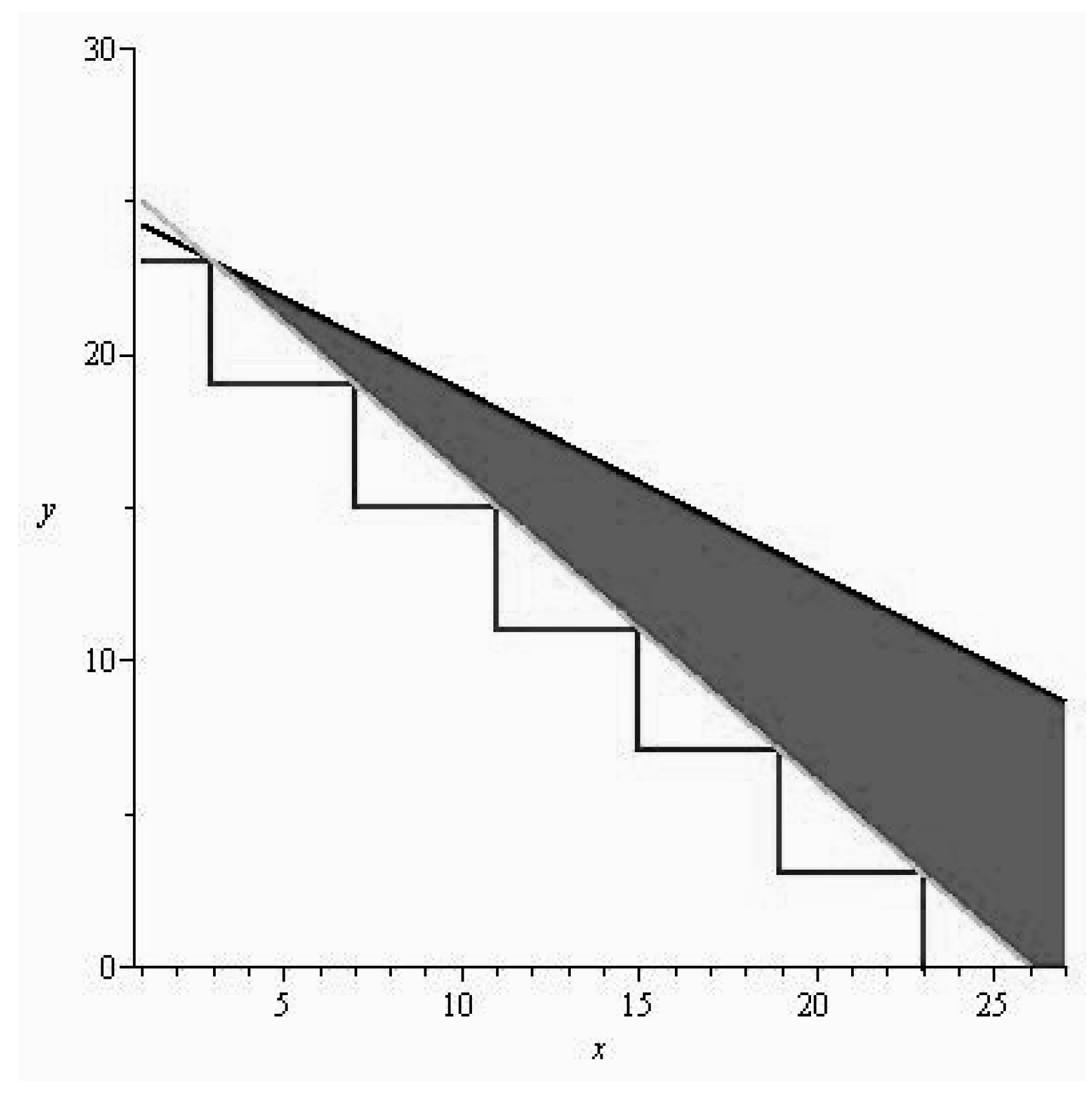
Lemma 2.

Let λ be the partition $\lambda =\left[{(\beta s+r)}^k,{((\beta -1)s+r)}^{\ell },\dots ,{(s+r)}^{\ell },0^{\ell +\alpha }\right]$, where α is an integer such that $0\le \alpha \le r\frac{\ell +1}{s-1}$. Consider another partition $\mu \subseteq \lambda$ such that there exists i satisfying $\langle \mu \rangle \left[i\right]=\langle \lambda \rangle \left[k\right]$. Then, $i=k$ and λ and μ have the same k first entries, i.e., $\mu \left[j\right]=\lambda \left[j\right]$, for $j=1,\dots ,k$.

Proof. 

First, we notice that ${\omega }_1^{\mu \left[i\right]}{u}^{\frac{1}{g}((N-i)(s-1)-\mu \left[i\right](\ell +1))}={\omega }_1^{\beta s+r}{u}^{\frac{1}{g}((s-1)(N-k)-(\beta s+r)(\ell +1)}$, which means that $(i,\mu [i\left]\right)$ lies on the line

$$\begin{array}{c}\hfill y=\beta s+r+\frac{s-1}{\ell +1}(k-x),\end{array}$$

(4)

and that ${\displaystyle k-i=\left(\mu \left[i\right]-(\beta s+r))\right)\frac{\ell +1}{s-1}}$. Since $\mu \subset \lambda$, $\mu \left[i\right]\le \beta s+r$ and, so, $k\le i$.

If $\lambda \left[i\right]>0$, then $i\le \beta \ell +k$ and the point $(i,\lambda [i\left]\right)$ lies on or below the line

$$\begin{array}{c}\hfill y=\beta s+r+\frac{s}{\ell }(k-x).\end{array}$$

(5)

Hence,

$$\begin{array}{c}\hfill 0\ge \mu \left[i\right]-\lambda \left[i\right]\ge \frac{s+\ell }{\ell (\ell +1)}(i-k),\end{array}$$

(6)

That is, $i\le k$ and, so, $i=k$.

Now, suppose that $i>k+(\beta -1)\ell$. In this case, $\mu \left[i\right]=0$ and, from Equation (4), we obtain

$$\begin{array}{c}\hfill i=k+(\beta s+r)\frac{\ell +1}{s-1}=r\frac{\ell +1}{s-1}+\beta +\frac{s}{s-1}(\ell +1)+k>r\frac{\ell +1}{s-1}+\beta \ell +k.\end{array}$$

Then, i is strictly greater than the size of $\mu$, which is impossible.

The only remaining possibility is $k=i$, and so $\mu \left[k\right]=\lambda \left[k\right]$. Since $\mu \subset \lambda$, we deduce also that $\mu \left[1\right]=\lambda \left[1\right]$, …, $\mu \left[k\right]=\lambda \left[k\right]$. □

Example 4.

In Figure 4, we illustrate the proof of Lemma 2 for the parameters $s=4$, $\ell =4$, $k=3$, $\beta =5$ and $r=3$. The shaded area illustrates the inequality in Equation (6), which is defined by the lines in Equations (4) (top) and (5) (bottom). Below it, we include the partition λ.

The following result shows that the reciprocal sum characterizes the quasistaircase partitions.

Proposition 4.

Consider a partition μ such that $\mu \subseteq QS(\ell ,k;s,r;\beta )$ and $⟅\mu ⟆=⟅QS(\ell ,k;s,r;\beta )⟆$. Then, $\mu =QS(\ell ,k;s,r;\beta )$.

Proof. 

Denote by $\lambda$ the quasistaircase partition, $\lambda =QS(\ell ,k;s,r;\beta )$. Then, there exists i such that $〈\mu 〉\left[i\right]=〈\lambda 〉\left[k\right]$. Otherwise, $\mu$ is completely contained in $\lambda$ and $⟅\mu ⟆=⟅QS(\ell ,k;s,r;\beta )⟆$ is impossible.

By Lemma 2, $i=k$ and $〈\mu 〉\left[j\right]=〈\lambda 〉\left[j\right]$, for $1\le j\le k$. Now, define two new partitions ${\lambda }^{\prime }$ and ${\mu }^{\prime }$ as the partitions obtained by deleting the first k entries of $\lambda$ and $\mu$, respectively. That is, ${\lambda }^{\prime }\left[j\right]=\lambda [j+k]$ and ${\mu }^{\prime }\left[j\right]=\mu [j+k]$, for $j\ge 1$. Then, either ${\lambda }^{\prime }=QS(l,l;s,r,\beta -1)$, and the above argument is applied to ${\alpha }^{\prime }$ and ${\mu }^{\prime }$, or else ${\lambda }^{\prime }=\left[0^{\ell +\alpha }\right]$, where $\alpha$ is defined in the statement of Lemma 2, and therefore ${\mu }^{\prime }=\left[0^{\ell +\alpha }\right]$. The proof is complete by noticing that the process must stop because $\lambda$ has only finitely many steps. □

Example 5.

The following table contains all the reciprocal sums ⟅μ⟆ associated to the partitions $\mu \subseteq \left[420\right]$:

⟅420⟆	⟅320⟆	⟅220⟆	⟅110⟆
$q^4{t}^2+q^{2}t+1$	$q^3{t}^2+q^{2}t+1$	$q^2{t}^2+q^{2}t+1$	$q{t}^2+qt+1$
⟅410⟆	⟅310⟆	⟅210⟆	⟅100⟆
$q^4{t}^3+qt+1$	$q^3{t}^2+qt+1$	$q^2{t}^2+qt+1$	$q{t}^2+t+1$
⟅400⟆	⟅300⟆	⟅200⟆	⟅000⟆
$q^4{t}^2+t+1$	$q^3{t}^2+t+1$	$q^2{t}^2+t+1$	$t^2+t+1$

Under the $(2,2)$-admissible specialization $(t,q)=(u,u^{-2})$, the table becomes:

⟅420⟆	⟅320⟆	⟅220⟆	⟅110⟆
$u^{-6}+u^{-3}+1$	$u^{-4}+u^{-3}+1$	$u^{-3}+u^{-2}+1$	$u^{-1}+2$
⟅410⟆	⟅310⟆	⟅210⟆	⟅100⟆
$u^{-6}+u^{-1}+1$	$u^{-4}+u^{-1}+1$	$u^{-2}+u^{-1}+1$	$2+u$
⟅400⟆	⟅300⟆	⟅200⟆	⟅000⟆
$u^{-6}+1+u$	$u^{-4}+1+u$	$u^{-2}+1+u$	$1+u+u^2$

We observe that the only partition whose reciprocal sum equals $u^{-6}+u^{-3}+1$ is $\left[420\right]$.

Notice that Proposition 4 can be alternatively stated as follows.

Corollary 2.

Suppose that $\mu \subseteq \lambda =QS(\ell ,k;s,r;\beta )$ is a partition such that $\langle \mu \rangle$ is a permutation of $\langle \lambda \rangle$. Then,

• $\mu =\lambda$,
• The intersection of the eigenspace of ξ with eigenvalue ${⟅\lambda ⟆}_{q^{-1},t^{-1}}$, and the space generated by $P_{\mu }$, with $\mu \subseteq \lambda$, has dimension 1.
• The intersection of the eigenspace of Ξ with eigenvalue ${⟅\lambda ⟆}_{q^{-1},t^{-1}}$, and the space generated by $M{S}_{\mu }$, with $\mu \subseteq \lambda$, has dimension 1.

Proof. 

It is easy to see that for a specialization of type $(t,q)=(u^b,{\omega }_1{u}^a)$ the following four assertions are equivalent: $\langle \mu \rangle$ is a permutation of $\langle \lambda \rangle$, ${\langle \mu \rangle }_{q^{-1},t^{-1}}$ is a permutation of ${\langle \lambda \rangle }_{q^{-1},t^{-1}}$, $⟅\mu ⟆=⟅\lambda ⟆$, and ${⟅\mu ⟆}_{q^{-1},t^{-1}}={⟅\lambda ⟆}_{q^{-1},t^{-1}}$. Proposition 4 allows us to complete the proof. □

5.3. On the Reciprocal Vector $\langle QS(\ell ,k;s,r;\beta )\rangle$

In this section, we prove that, under a $(s,\ell )$-admissible specialization, all the entries of $\langle QS(\ell ,k;s,r;\beta )\rangle$ are distinct. For simplicity, we denote $QS\left(\ell ,k;s,r;\beta \right)$ by $\lambda$ and the specialization $(t,q)=\left(u^{\frac{s-1}{g}},{\omega }_1{u}^{-\frac{\ell +1}{g}}\right)$ by $(t,q)=\left(u^b,{\omega }_1{u}^{-a}\right)$.

Define the utility function $h\left(w,z\right)=bz-aw$, so that, for a partition $\mu$, $〈\mu 〉\left[i\right]={\omega }_1^{\mu \left[i\right]}{u}^{h\left(\mu \left[i\right],N-i\right)}$. Define also a decreasing sequence as $j_1=N-n_0$, with $n_0=(\ell +1)\frac{r}{s-1}+\ell$; $j_m=k+\left(\beta -m+1\right)\ell$, for $2\le m\le \beta +1$; and $j_{\beta +2}=0$. Notice this sequence splits the interval $[0,N]$ into $\beta +2$ pieces.

If $j_{m+1}<i\le j_m$, for $1\le m\le \beta +1$, then $\lambda \left[i\right]=r+ms$ and $〈\lambda 〉\left[i\right]={\omega }_1^{r+ms}{u}^{h\left(r+ms,N-i\right)}$. If $j_1<i\le N$, $\lambda \left[i\right]=0$ and $〈\lambda 〉\left[i\right]=u^{h\left(0,N-i\right)}$.

Let $c\in \mathbb{N}$ such that $n_0=\left(\ell +1\right)c-1$ and $r=(s-1)(c-1)$. Then,

$$\begin{array}{c}\hfill \begin{array}{c}-\frac{m\left(s+\ell \right)}{g}=h\left(r+ms,N-j_m\right)\le h\left(r+ms,N-i\right)\le h\left(r+ms,N-j_m+\ell -1\right)\hfill \\ =\frac{1}{g}\left[-m\left(s+\ell \right)+\left(s-1\right)\left(\ell -1\right)\right].\hfill \end{array}\end{array}$$

(7)

Here is an example showing that the utility function h alone does not suffice to separate the $〈\lambda 〉$ values.

Example 6.

Let $\ell =5,s=3,N=15,n_0=5$. Then, $g=2$, $r=0$, and the relation $15=k+10\beta$ implies that $k=5$ and $\beta =1$. This corresponds to the quasistaircase partition $\lambda =\left[6^5,3^5,0^5\right]$, for which the values of the sequence are $j_1=10$, $j_2=5$ and $j_3=0$. Then, the vector of values of $h\left(\lambda \right[i],N-i)$ is

$$\begin{array}{c}\hfill \left[-4,-5,-6,-7,-8,0,-1,-2,-3,-4,4,3,2,1,0\right].\end{array}$$

There are two pairs of equal entries, however the corresponding entries of $〈\lambda 〉$ are different. For the value 0, $〈\lambda 〉\left[6\right]={\omega }^3\ne 1=〈\lambda 〉\left[15\right]$, where $\omega =-1$. In addition, for the value $-4$, $〈\lambda 〉\left[1\right]={\omega }^6{u}^{-4}\ne {\omega }^3{u}^{-4}=〈\lambda 〉\left[10\right]$.

Proposition 5.

The entries of $〈\lambda 〉$ are pairwise distinct.

Proof. 

Take two indices $i_1$ and $i_2$ and assume without lost of generality that $1\le i_1<i_2\le N$. We check that the values of $〈\lambda 〉\left[i_1\right]$ and $〈\lambda 〉\left[i_2\right]$ are distinct. For that, it is enough to check that $h(\lambda \left[i_1\right],N-i_1)\ne h(\lambda \left[i_2\right],N-i_2)$ or $h(\lambda \left[i_1\right],i_1)\ne h(\lambda \left[i_2\right],i_2)$. Let us analyze the differences by looking at the indices in the division of the interval $[1,N]$ given by the sequence $\left\{j_m\right\}$.

If $j_{m+1}<i_1<i_2\le j_m$, then $h\left(r+ms,N-i_1\right)-h\left(r+ms,N-i_2\right)=b\left(i_2-i_1\right)>0$. Thus, $〈\lambda 〉\left[i_1\right]\ne 〈\lambda 〉\left[i_2\right]$. The same happens if $j_1<i_1<i_2\le N$ since $h\left(0,N-i_1\right)-h\left(0,N-i_2\right)=b\left(i_2-i_1\right)>0$.

Now, suppose $j_{m_1+1}<i_1\le j_{m_1}\le j_{m_2+1}<i_2\le j_{m_2}$, then (7) shows that

$$\begin{array}{c}\hfill h\left(r+m_{2}s,i_2\right)-h\left(r+m_{1}s,i_1\right)\ge \frac{1}{g}\left\{\left(m_1-m_2\right)\left(s+\ell \right)-\left(s-1\right)\left(\ell -1\right)\right\}.\end{array}$$

Thus, if $m_1-m_2>{\displaystyle \frac{\left(s-1\right)\left(\ell -1\right)}{s+\ell }}$, then $〈\lambda 〉\left[i_1\right]\ne 〈\lambda 〉\left[i_2\right]$.

Consider the case $1\le m_1-m_2\le {\displaystyle \frac{\left(s-1\right)\left(\ell -1\right)}{s+\ell }}$; then, $〈\lambda 〉\left[i_1\right]={\omega }_1^{r+m_{1}s}{u}^{h\left(r+m_{1}s,N-i_1\right)}$ and $〈\lambda 〉\left[i_2\right]={\omega }_1^{r+m_{2}s}{u}^{h\left(r+m_{2}s,N-i_2\right)}$. There are two different arguments depending on whether ${\omega }_1\ne 1$.

If ${\omega }_1\ne 1$, suppose that ${\displaystyle 1=\frac{〈\lambda 〉\left[i_1\right]}{〈\lambda 〉\left[i_2\right]}=q^{\left(m_1-m_2\right)s}{t}^{i_2-i_1}}$. By Lemma 1, $\left(m_1-m_2\right)s=p\left(s-1\right)$, for some $p\in \mathbb{N}$, but $1\le m_1-m_2\le {\displaystyle \frac{\left(s-1\right)\left(\ell -1\right)}{s+\ell }}<s-1$ and $\gcd \left(s,s-1\right)=1$, which is a contradiction.

If ${\omega }_1=1$, or equivalently $\gcd \left(s-1,\ell +1\right)=1$, then $h\left(\lambda \left[i\right],N-i\right)\equiv -\left(\ell +1\right)\lambda \left[i\right]\mathrm{mod}\left(s-1\right)$. If $j_{m+1}<i\le j_m$, then $h\left(\lambda \left[i\right],N-i\right)\equiv m\left(s+\ell \right)\mathrm{mod}\left(s-1\right)$ and $\gcd \left(s+\ell ,s-1\right)=1$. In the case $j_{m_1+1}<i_1\le j_{m_1}\le j_{m_2+1}<i_2\le j_{m_2}$, with $1\le m_1-m_2\le {\displaystyle \frac{\left(s-1\right)\left(\ell -1\right)}{s+\ell }}$, it follows that

$$\begin{array}{c}\hfill h\left(r+m_{2}s,i_2\right)-h\left(r+m_{1}s,i_1\right)\equiv \left(m_1-m_2\right)\left(s+\ell \right)\mathrm{mod}\left(s-1\right).\end{array}$$

This implies $h\left(r+m_{2}s,i_2\right)-h\left(r+m_{1}s,i_1\right)\not\equiv 0\mathrm{mod}\left(s-1\right)$, since $1\le m_1-m_2<s-1$. The similar argument applies when $j_1<i_2\le N$.

Suppose $j_{m+1}=j_m<i_1\le j_m$ and $j_1<i_2\le N$. By (7), and the fact that $h\left(0,N-i_2\right)\ge 0$,

$$\begin{array}{c}\hfill h\left(0,N-i_2\right)-h\left(r+m_{1}s,N-i_1\right)\ge -h\left(r+m_{1}s,N-j_{m_1}+\ell -1\right)=\frac{1}{g}\left\{m_1\left(s+\ell \right)-\left(s-1\right)\left(\ell -1\right)\right\}.\end{array}$$

If $m_1>\frac{\left(s-1\right)\left(\ell -1\right)}{s+\ell }$, then $h\left(0,N-i_2\right)-h\left(r+m_{1}s,N-i_1\right)>0$ and $〈\lambda 〉\left[i_1\right]\ne 〈\lambda 〉\left[i_2\right]$. Otherwise, suppose ${\displaystyle 1=\frac{〈\lambda 〉\left[i_1\right]}{〈\lambda 〉\left[i_2\right]}=q^{m_{1}s+r}{t}^{i_2-i_1}}$ and $m_{1}s+r=p\left(s-1\right)$. Then, $m_{1}s=\left(s-1\right)\left(p-c+1\right)$, which is impossible for $1\le m_1<s-1.$ □

6. Factorizations and Wheel Condition

In this section, we investigate the case of the staircase partitions that are a particular case of quasistaircase partitions of the form

$$\begin{array}{c}\hfill St(\ell ,k;s;\beta ):=QS(\ell ,k;s,0;\beta )=[{\left((\beta +1)s\right)}^k,{\left(\beta s\right)}^{\ell },\dots ,s^{\ell },0^{\ell }],\end{array}$$

for any $\ell \ge 1$, $0\le k<\ell$, $s\ge 2$ and $\beta \ge 1$. We also assume that the parameters q and t specialize as

$$\begin{array}{c}\hfill (t,q)=\left(u^{\frac{s-1}{g}},{\omega }_1{u}^{-\frac{\ell +1}{g}}\right),\end{array}$$

where $g=\gcd (\ell +1,s-1)$ and ${\omega }_1^{\frac{s-1}{g}}$ is a primitive gth root of the unity.

6.1. Wheel Condition and Admissible Partitions

We start recalling the main results of [10].

Definition 7.

A symmetric polynomial $p(x_1,\dots ,x_N)$ satisfies the $(s,\ell )$-wheel condition if

$$\begin{array}{c}\hfill \left\{\frac{x_2}{x_1},\dots ,\frac{x_{\ell +1}}{x_{\ell }},\frac{x_1}{x_{\ell +1}}\right\}\subset \{t,tq,\dots ,t{q}^{s-1}\}\end{array}$$

implies that $p(x_1,\dots ,x_N)=0$. It is easy to check that the set of the symmetric polynomials satisfying the wheel condition is an ideal, denoted by $J_N^{\ell ,s}$ in [10]. A$(\ell ,s,N)$-admissible partition is a partition $\lambda =[{\lambda }_1,\dots ,{\lambda }_N]$ satisfying ${\lambda }_i-{\lambda }_{i+\ell }\ge s$ for any $i=1,\dots ,N-\ell$.

The following theorem summarizes two results that relates both concepts.

Theorem 1

([10]). The ideal $J_N^{\ell ,s}$ is generated by the Macdonald polynomials indexed by admissible partitions,

$$\begin{array}{c}\hfill J_N^{\ell ,s}=\mathrm{span}\left\{P_{\lambda }({\mathbb{X}}_N;q,t):\lambda is(\ell ,s,N)\text{-}admissiblepartition\right\}.\end{array}$$

Moreover, $J_N^{\ell ,s}$ is stable under the action of $L_{q,t}^{+}=(1-q)(\xi -\Xi )$.

Remarking that $P_{St(\ell ,k;s;\beta )}({\mathbb{X}}_{(\beta +1)\ell +k};q,t)$ is a minimal degree polynomial belonging to $J_{(\beta +1)\ell +k}^{\ell ,s}$, by applying Theorem 1 we get the following result.

Proposition 6.

$$\begin{array}{c}\hfill P_{St(\ell ,k;s;\beta )}({\mathbb{X}}_{(\beta +1)\ell +k};q,t)\stackrel{(\ast )}{=}M{S}_{St(\ell ,k;s;\beta )}({\mathbb{X}}_{(\beta +1)\ell +k};q,t).\end{array}$$

Proof. 

Since $M{S}_{St(\ell ,k;s;\beta )}({\mathbb{X}}_{(\beta +1)\ell +k};q,t)$ is in the kernel of $L_{q,t}^{+}$, $P_{St(\ell ,k;s;\beta )}({\mathbb{X}}_{(\beta +1)\ell +k};q,t)$ and $M{S}_{St(\ell ,k;s;\beta )}({\mathbb{X}}_{(\beta +1)\ell +k};q,t)$ are in the same eigenspace of $\xi$ with reciprocal sum

$$\begin{array}{c}\hfill ⟅St(\ell ,k;s;\beta )⟆=q^{(\beta +1)s}·\left(\sum _{i=1}^k{t}^{N-i+1}\right)+\sum _{j=0}^{\beta }{q}^{js}·\left(\sum _{i=1}^{\ell }{t}^{N-k-(\beta -j)\ell -i+1}\right).\end{array}$$

Recall that, for some coefficients $c_{\mu }(q,t)$,

$$\begin{array}{c}\hfill M{S}_{St(\ell ,k;s;\beta )}\stackrel{(\ast )}{=}{P}_{St(\ell ,k;s;\beta )}+\sum _{\mu \subset St(\ell ,k;s;\beta )}{c}_{\mu }(q,t)·P_{\mu }.\end{array}$$

Consider the spaces generated by the polynomials $P_{\mu }$, with $\mu \subseteq St(\ell ,k;s;\beta )$. This space splits into several eigenspaces, and each of them is associated with a reciprocal sum $⟅\mu ⟆$. From Corollary 2, the subspace of the eigenspace associated with the reciprocal sum $⟅St(\ell ,k;s;\beta )⟆$ generated by the polynomials $M{S}_{\mu }$, with $\mu \subseteq St(\ell ,k;s;\beta )$, has dimension 1. Therefore, $P_{St(\ell ,k;s;\beta )}({\mathbb{X}}_{(\beta +1)\ell +k};q,t)$ and $M{S}_{St(\ell ,k;s;\beta )}({\mathbb{X}}_{(\beta +1)\ell +k};q,t)$ are proportional. □

Example 7.

For instance, observe that the shifted Macdonald polynomial

$$\begin{array}{c}\hfill M{S}_{\left[20\right]}\left(x_1,x_2;q=\frac{1}{u},t=u^2\right)=\frac{\left(x_2{x}_{1}u+x_1^{2}u+x_2^{2}u-\frac{x_2{x}_1}{u}+x_1{u}^2{x}_2-x_1^2-x_2^2-x_2{x}_1\right)}{\left(1-u^{-2}\right){\left(1-u^{-1}\right)}^2}\end{array}$$

is homogeneous and equal to $P_{\left[20\right]}\left(x_1,x_2;q=\frac{1}{u},u^2\right)$ up to a multiplicative factor.

6.2. Factorizations

From Proposition 6, the polynomial $M{S}_{St(\ell ,k;s;\beta )}$ is homogeneous for $(\ell ,s)$-admissible specializations. Moreover,

$$\begin{array}{c}\hfill M{S}_{St(\ell ,k;s;\beta )}\left({\mathbb{X}}_{k+\beta \ell }+\frac{1-t^{\ell }}{1-t}y;q,t\right)=y^{\frac{\ell s\beta (\beta -1)}{2}+ks(\beta +1)}M{S}_{St(\ell ,k;s;\beta )}\left(\frac{{\mathbb{X}}_{k+\beta \ell }}{y}+\frac{1-t^{\ell }}{1-t};q,t\right).\end{array}$$

Applying Proposition 3,

$$\begin{array}{c}\hfill {\displaystyle M{S}_{St(\ell ,k;s;\beta )}\left({\mathbb{X}}_{k+\beta \ell }+\frac{1-t^{\ell }}{1-t};q,t\right)\stackrel{(\ast )}{=}\mathcal{R}\left({\mathbb{X}}_{\beta \ell +k};t^{\ell }\frac{1-q^s}{1-q}\right)M{S}_{St(\ell ,k;s;\beta -1)}\left(q^{-s}{t}^{-\ell }{\mathbb{X}}_{k+\beta \ell };q,t\right).}\end{array}$$

Again, Proposition 6 shows that the polynomial $M{S}_{St(\ell ,k;s;\beta -1)}\left({\mathbb{X}}_{k+\beta \ell };q,t\right)$ is homogeneous.

Proposition 7.

$$\begin{array}{c}\hfill {\displaystyle M{S}_{St(\ell ,k;s;\beta )}\left({\mathbb{X}}_{k+\beta \ell }+\frac{1-t^{\ell }}{1-t}y;q,t\right)\stackrel{(\ast )}{=}\mathcal{R}\left({\mathbb{X}}_{k+\beta \ell };y{t}^{\ell }\frac{1-q^s}{1-q}\right)M{S}_{St(\ell ,k;s;\beta -1)}\left(q^{-s}{t}^{-\ell }{\mathbb{X}}_{k+\beta \ell };q,t\right).}\end{array}$$

Example 8.

Consider the partition $\left[42200\right]=St(2,1;2;1)$ and the specialization $(t,q)=(u,u^{-3})$. Then,

$$\begin{array}{c}\hfill \frac{M{S}_{\left[42200\right]}(x_1,x_2,x_3,yt,y)}{M{S}_{\left[200\right]}(q^{-2}{t}^{-2}{x}_1,q^{-2}{t}^{-2}{x}_2,q^{-2}{t}^{-2}{x}_3)}\stackrel{(\ast )}{=}\prod _{i=1}^3(x_i-u^{2}y)(x_1-u^{-1}y).\end{array}$$

Set ${\mathbb{Y}}_{i,\beta }=y_i+y_{i+1}+\cdots +y_{\beta }$, for any $0\le i\le \beta$, and consider the polynomial which is symmetric in both alphabets ${\mathbb{X}}_k$ and ${\mathbb{Y}}_{0,\beta }$:

$$\begin{array}{c}\hfill {\mathcal{P}}_{\ell ,k;s;\beta }({\mathbb{X}}_k;{\mathbb{Y}}_{0,\beta }):=M{S}_{St(\ell ,k;s;\beta )}\left({\mathbb{X}}_k+\frac{1-t^{\ell }}{1-t}{\mathbb{Y}}_{0,\beta };q,t\right).\end{array}$$

By Proposition 7,

$$\begin{array}{c}\hfill {\displaystyle {\mathcal{P}}_{St(\ell ,k;s;\beta )}({\mathbb{X}}_k;{\mathbb{Y}}_{0,\beta })\stackrel{(\ast )}{=}\mathcal{R}\left({\mathbb{X}}_k+\frac{1-t^{\ell }}{1-t}{\mathbb{Y}}_{1,\beta };t^{\ell }\frac{1-q^s}{1-q}{y}_0\right){\mathcal{P}}_{St(\ell ,k;s;\beta -1)}(q^{-s}{t}^{\ell }{\mathbb{X}}_k;q^{-s}{t}^{\ell }{\mathbb{Y}}_{1,\beta }).}\end{array}$$

Iterating, one finds

$$\begin{array}{ccc}\hfill {\mathcal{P}}_{St(\ell ,k;s;\beta )}({\mathbb{X}}_k;{\mathbb{Y}}_{0,\beta })& {\displaystyle \stackrel{(\ast )}{=}}& {\displaystyle \prod _{\alpha =0}^{\beta -1}\mathcal{R}\left({\mathbb{X}}_k+\frac{1-t^{\ell }}{1-t}{\mathbb{Y}}_{\alpha +1,\beta };t^{\ell }\frac{1-q^s}{1-q}{y}_{\alpha }\right){\mathcal{P}}_{St(\ell ,k;s;0)}(q^{-\beta s}{t}^{-\beta \ell }{\mathbb{X}}_k;y_{\beta }{q}^{-\beta s}{t}^{-\beta \ell }),}\hfill \\ \hfill \mathrm{with}{\mathcal{P}}_{St(\ell ,k;s;0)}({\mathbb{X}}_k;y_{\beta })& =& M{S}_{St(\ell ,k;s;0)}\left({\mathbb{X}}_k+y_{\beta }\frac{1-t^{\ell }}{1-t};q,t\right).\hfill \end{array}$$

Once again, applying Propositions 6 and 3, one gets the following result.

Theorem 2.

$$\begin{array}{c}{\displaystyle {\mathcal{P}}_{St(\ell ,k;s;\beta )}({\mathbb{X}}_k;{\mathbb{Y}}_{0,\beta })\stackrel{(\ast )}{=}\prod _{\alpha =0}^{\beta }\mathcal{R}\left({\mathbb{X}}_k+\frac{1-t^{\ell }}{1-t}{\mathbb{Y}}_{\alpha +1,\beta };t^{\ell }\frac{1-q^s}{1-q}{y}_{\alpha }\right)}\hfill \\ \hfill {\displaystyle =\prod _{\alpha =0}^{\beta }\prod _{j=0}^{s-1}\left[\prod _{i=1}^k(x_i-t^{\ell }{q}^j{y}_{\alpha })\prod _{i=\alpha +1}^{\beta }\prod _{a=0}^{\ell -1}(t^a{y}_i-t^{\ell }{q}^j{y}_{\alpha })\right].}\end{array}$$

Example 9.

For $(t,q)=(u,u^{-3})$, we have

$$\begin{array}{c}{\displaystyle M{S}_{\left[42200\right]}(x_1,t{y}_1,y_1,t{y}_0,y_0)\stackrel{(\ast )}{=}(x_1-u^2{y}_0)(x_1-u^{-1}{y}_0)(x_1-u^2{y}_1)(x_1-u^{-1}{y}_1)}\hfill \\ \hfill \times (y_1-u^2{y}_0)(y_1-u^{-1}{y}_0)(u{y}_1-u^2{y}_0)(u{y}_1-u^{-1}{y}_0).\end{array}$$

7. Beyond the Wheel Condition

First, we recall that, for some specializations of $(q,t)$, the quasistaircase polynomials satisfy the HW condition, [11]. Using an argument of dimension of eigenspaces, we show that the shifted Macdonald are homogeneous.

Theorem 3

([11]). For β, s, r, k, $\ell \in \mathbb{N}$, with $k\le \ell$, consider $\lambda =[{((\beta +1)s+r)}^k,{(\beta s+r)}^{\ell },\dots ,{(s+r)}^{\ell }]$ and the specialization

$$\begin{array}{c}\hfill (t,q)=\left(u^{\frac{s-1}{g}},u^{-\frac{\ell +1}{g}}{\omega }_1\right),\end{array}$$

where $g=\gcd (\ell +1,s-1)$ and ${\omega }_1$ is a rth root of the unity such that ${\omega }_1^{\frac{s-1}{g}}$ is a gth primitive root of the unity. The polynomial $P_{\lambda }(x_1+\cdots +x_n;q,t)$ is in the kernel of $L_{q,t}^{+}$ when $n=\frac{\ell +1}{s-1}r+\ell (\beta +1)+k$ is an integer.

The shifted symmetric polynomial $M{S}_{QS(\ell ,k;s,r;\beta )}$ is an eigenfunction of $\Xi$ having the same eigenvalue as $P_{QS(\ell ,k;s,r;\beta )}$. However, from Corollary 2, the corresponding eigenspace has dimension 1, which proves the following result.

Corollary 3.

$$P_{QS(\ell ,k;s,r;\beta )}(\mathbb{X};q,t)\stackrel{(\ast )}{=}M{S}_{QS(\ell ,k;s,r;\beta )}(\mathbb{X};q,t).$$

Moreover, this implies that $M{S}_{QS(\ell ,k;s,r;\beta )}(\mathbb{X};q,t)$ is homogeneous.

By Corollary 3, we have

$$\begin{array}{c}M{S}_{QS(\ell ,k;s,r;\beta )}\left({\displaystyle {\mathbb{X}}_{k+\beta \ell }+\frac{1-t^{r\frac{\ell +1}{s-1}+\ell }}{1-t}{y}_{\beta };q,t}\right)\hfill \\ \hfill =y_{\beta }^{\frac{1}{2}(\beta +1)(\ell \beta +2k)s+r(k+l\beta )}M{S}_{QS(\ell ,k;s,r;\beta )}\left({\displaystyle \frac{{\mathbb{X}}_{k+\beta \ell }}{y_{\beta }}+\frac{1-t^{r\frac{\ell +1}{s-1}+\ell }}{1-t};q,t}\right).\end{array}$$

Applying Proposition 3, we obtain

$$\begin{array}{c}{\displaystyle M{S}_{QS(\ell ,k;s,r;\beta )}\left({\mathbb{X}}_{k+\beta \ell }+\frac{1-t^{r\frac{\ell +1}{s-1}+\ell }}{1-t};q,t\right)\stackrel{(\ast )}{=}}\hfill \\ \hfill {\displaystyle \mathcal{R}\left({\mathbb{X}}_{k+\beta \ell };t^{\frac{\ell +1}{s-1}r+\ell }\frac{1-q^{s+r}}{1-q}\right)M{S}_{QS(\ell ,k;s,0;\beta )}\left(q^{-r-s}{t}^{-r\frac{\ell +1}{s-1}-\ell }{\mathbb{X}}_{k+\beta \ell };q,t\right).}\end{array}$$

Again, by Corollary 3, $M{S}_{QS(\ell ,k;s,0;\beta )}$ is an homogeneous polynomial, and then,

$$\begin{array}{c}\hfill \begin{array}{c}{\displaystyle M{S}_{QS(\ell ,k;s,r;\beta )}\left({\displaystyle {\mathbb{X}}_{k+\beta \ell }+\frac{1-t^{r\frac{\ell +1}{s-1}+\ell }}{1-t}{y}_{\beta };q,t}\right)\stackrel{(\ast )}{=}}\hfill \\ \mathcal{R}\left({\mathbb{X}}_{k+\beta \ell };t^{\frac{\ell +1}{s-1}r+\ell }\frac{1-q^{s+r}}{1-q}{y}_{\beta }\right)M{S}_{QS(\ell ,k;s,0;\beta -1)}\left(q^{-r-s}{t}^{-r\frac{\ell +1}{s-1}-\ell }{\mathbb{X}}_{k+\beta \ell };q,t\right).\hfill \end{array}\end{array}$$

(8)

Theorem 2 completes the proof of the following theorem.

Theorem 4.

$$\begin{array}{c}{\displaystyle M{S}_{QS(\ell ,k;s,r;\beta )}\left({\mathbb{X}}_k+\frac{1-t^{\ell }}{1-t}{\mathbb{Y}}_{0,\beta -1}+\frac{1-t^{r\frac{\ell +1}{s-1}+\ell }}{1-t}{y}_{\beta };q,t\right)\stackrel{(\ast )}{=}}\hfill \\ \hfill \mathcal{R}\left({\mathbb{X}}_k+\frac{1-t^{\ell }}{1-t}{\mathbb{Y}}_{0,\beta -1};t^{\frac{\ell +1}{s-1}r+\ell }\frac{1-q^{s+r}}{1-q}{y}_{\beta }\right)\prod _{\alpha =0}^{\beta -1}\mathcal{R}\left({\mathbb{X}}_k+\frac{1-t^s}{1-t}{\mathbb{Y}}_{\alpha +1,\beta -1};t^{\ell }\frac{1-q^s}{1-q}{y}_{\alpha }\right).\end{array}$$

Let us show this result with an example.

Example 10.

For $(t,q)=(u,u^{-3})$,

$$\begin{array}{c}M{S}_{\left[533\right]}(x_1+(1+t)y_0+(1+t+t^2+t^3+t^4)y_1;q=u^{-3},t=u)\hfill \\ {\displaystyle \stackrel{(\ast )}{=}\mathcal{R}(x_1+(1+t)y_0;t^5(1+q+q^2)y_1)M{S}_2(x_1+(1+t)y_0;q=u^{-3},t=u)\stackrel{(\ast )}{=}}\\ \hfill \mathcal{R}(x_1+(1+t)y_0;t^5(1+q+q^2)y_1)\mathcal{R}(x_1;t^2(1+q)y_0)\\ \hfill {\displaystyle =\prod _{i=0}^2\left[(x_1-t^5{q}^i{y}_1)(y_0-t^5{q}^i{y}_1)(t{y}_0-t^5{q}^i{y}_1)\right](x_1-t^2{y}_0)(x_1-t^{2}q{y}_0).}\end{array}$$

8. Conclusions and Perspectives

In this last section, we explore the second clustering property conjectured by Bernevig and Haldane and we present some examples that illustrate future work that can be done in this direction.

8.1. The Second Clustering Property

Most of the different variants of Macdonald polynomials presented in this paper specialize to Jack polynomials by sending u to 1 when $\ell +1$ and $s-1$ are coprime, which corresponds to setting $t=q^{\alpha }$ and sending $\alpha$ to 1. Moreover, this implies also that $s-1$ divides r. In that context, Proposition 7 gives that

$$\begin{array}{c}\hfill J_{St(\ell ,k;s;\beta )}^{\left(-\frac{\ell +1}{s-1}\right)}\left({\mathbb{X}}_{k+\beta \ell }+\ell y\right)\stackrel{(\ast )}{=}\prod _{i=1}^{\beta \ell }{(x_i-y)}^s{J}_{St(\ell ,k;s;\beta -1)}^{\left(-\frac{\ell +1}{s-1}\right)}\left({\mathbb{X}}_{k+\beta \ell }\right).\end{array}$$

By Equation (8),

$$\begin{array}{c}\hfill J_{QS(\ell ,k;s,r;\beta )}^{\left(-\frac{\ell +1}{s-1}\right)}\left({\mathbb{X}}_{k+\beta \ell }+\left(r\frac{\ell +1}{s-1}+\ell \right)y\right)\stackrel{(\ast )}{=}\prod _{i=1}^{\beta \ell }{(x_i-y)}^{s+r}{J}_{St(\ell ,k;s;\beta -1)}^{\left(-\frac{\ell +1}{s-1}\right)}\left({\mathbb{X}}_{k+\beta \ell }\right).\end{array}$$

(9)

The fact that ${\displaystyle \prod _{i=1}^{\beta \ell }{(x_i-y)}^{s+r}}$ divides the polynomial $J_{QS(\ell ,k;s,r;\beta )}^{\left(-\frac{\ell +1}{s-1}\right)}\left({\mathbb{X}}_{k+\beta \ell }+\left(r\frac{\ell +1}{s-1}+\ell \right)y\right)$ is a special case of a result of [4] [Theorem 1.1]. The following table contrasts Bernevig and Haldane notation (B-H notation) with our notation in order to transcribe the second clustering property into our notation.

Our notation	B-H notation
ℓ	k
k	0
s	r
$\frac{r}{s-1}+1$	s
$s+r$	$s(r-1)+1$
$St(\ell ,0;s;\beta )$	${\lambda }_{k,r,1}^{\beta }$
$QS(\ell ,0;s,r;\beta )$	${\lambda }_{k,r,s}^{\beta }$
$r\frac{\ell +1}{s-1}+\ell$	$n_0$
${\mathbb{X}}_{k+\beta \ell }$	$z_{n_0+1}+\cdots +z_N$
y	$Z=z_1=\cdots =z_{n_0}$

We recover the equality in Equation (1) by setting $k=0$ in Equation (9). This proves the second clustering property conjectured by Bernevig and Haldane [2]. Furthermore, Equation (8) is more general than those conjectured in [2] for two reasons. First, we consider quasistaircase partitions $QS(\ell ,k;s,r;\beta )$, with $0\le k<\ell$, while only the case $k=0$ was investigated in [1,2]. It should be interesting to know if some of these polynomials can be interpreted as wave functions in FQHT. In addition, when ${\omega }_1\ne 1$, the Macdonald polynomial does not degenerate to a Jack polynomial when u tends to 1.

More generally, the following equality is obtained from Theorem 4:

$$\begin{array}{c}{\displaystyle J_{QS(\ell ,k;s,r;\beta )}^{\left(-\frac{\ell +1}{s-1}\right)}\left({\mathbb{X}}_k+\ell {\mathbb{Y}}_{0,\beta -1}+\left(r\frac{\ell +1}{s-1}+\ell \right)y_{\beta }\right)\stackrel{(\ast )}{=}}\hfill \\ \hfill \prod _{i=1}^k{(x_i-y_{\beta })}^{r+s}\prod _{\alpha =0}^{\beta }\left[{(y_{\alpha }-y_{\beta })}^{(s+r)\ell }\prod _{i=1}^k{(x_i-y_{\alpha })}^s\prod _{i=\alpha +1}^{\beta -1}{(y_i-y_{\alpha })}^{\ell s}\right].\end{array}$$

We finish this subsection by presenting more general identities involving partitions which are not quasistaircase for the considered specialization. For instance,

$$\begin{array}{c}\hfill {\displaystyle J_{\left[43210\right]}^{(-3)}(x+2y_1+2y_2)\stackrel{(\ast )}{=}{y}_1{y}_2{(y_1-y_2)}^4{(x-y_1)}^2{(x-y_2)}^2.}\end{array}$$

This formula is in fact a specialization of

$$\begin{array}{c}{P}_{\left[43210\right]}\left(x+(1+t)y_1+(1+t)y_2;q=t^{-3},t\right)\hfill \\ \hfill {\displaystyle \stackrel{(\ast )}{=}{y}_1{y}_2(y_1-t{y}_2)(y_1-t^2{y}_2)(y_2-t{y}_1)(y_2-t^2{y}_1)(tx-y_1)(x-t^2{y}_1)(tx-y_2)(x-t^2{y}_2).}\end{array}$$

Notice that this polynomial does not satisfy the HW condition. This suggests that there exists a Macdonald version of the result of [4], Theorem 1.1.

8.2. Other Clustering and Factorizations Properties

The first and third clustering conjectures suggest that there exist many ways to factorize HW Macdonald polynomials by specializing the variables involved. Let us illustrate this remark by giving an example.

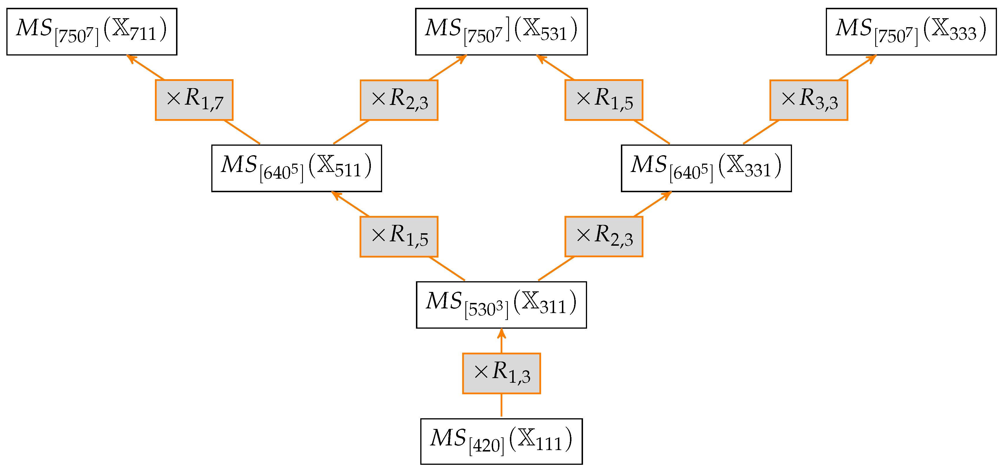
For a partition $\lambda =[{\lambda }_1,{\lambda }_2,{\lambda }_3]$, consider the alphabet ${\mathbb{X}}_{\lambda }=\frac{1-u^{{\lambda }_1}}{1-u}{x}_1+\frac{1-u^{{\lambda }_2}}{1-u}{x}_2+\frac{1-u^{{\lambda }_3}}{1-u}{x}_3$. Let ${\rho }_i$ be the operator that adds 2 to the ith entry of $\lambda$ if, after this operation, the resulting vector is still a partition. We set also ${\displaystyle R_{i;k}=\prod _{\genfrac{}{}{0pt}{}{1\le j\le N}{j\ne i}}(u^k{x}_i-x_j)}$.

Starting with $M{S}_{\left[420\right]}({\mathbb{X}}_{111};q=u^{-2},t=u)$, and by ${\mathbb{X}}_{111}{\rho }_1={\mathbb{X}}_{311}$, one obtains

$$\begin{array}{c}\hfill M{S}_{\left[{530}^4\right]}({\mathbb{X}}_{311};q=u^{-2},t=u)=R_{1;3}M{S}_{\left[420\right]}({\mathbb{X}}_{111};q=u^{-2},t=u).\end{array}$$

The next step is more interesting because there are two kinds of specializations that provide nice factorizations:

$$\begin{array}{ccc}\hfill M{S}_{\left[{640}^6\right]}({\mathbb{X}}_{511};q=u^{-2},t=u)& {\displaystyle \stackrel{(\ast )}{=}}& R_{1;5}M{S}_{\left[{530}^4\right]}({\mathbb{X}}_{311};q=u^{-2},t=u),\mathrm{and}\hfill \\ \hfill M{S}_{\left[{640}^6\right]}({\mathbb{X}}_{331};q=u^{-2},t=u)& {\displaystyle \stackrel{(\ast )}{=}}& R_{2;3}M{S}_{\left[{530}^4\right]}({\mathbb{X}}_{311};q=u^{-2},t=u).\hfill \end{array}$$

Continuing, we get other new nice factorizations:

$$\begin{array}{ccc}\hfill M{S}_{\left[{750}^8\right]}({\mathbb{X}}_{711};q=u^{-2},t=u)& {\displaystyle \stackrel{(\ast )}{=}}& R_{1;7}M{S}_{\left[{640}^4\right]}({\mathbb{X}}_{511};q=u^{-2},t=u),\hfill \\ \hfill M{S}_{\left[{750}^8\right]}({\mathbb{X}}_{333};q=u^{-2},t=u)& {\displaystyle \stackrel{(\ast )}{=}}& R_{3;3}M{S}_{\left[{640}^4\right]}({\mathbb{X}}_{331};q=u^{-2},t=u),\hfill \\ \hfill M{S}_{\left[{750}^8\right]}({\mathbb{X}}_{531};q=u^{-2},t=u)& {\displaystyle \stackrel{(\ast )}{=}}& R_{2;3}M{S}_{\left[{640}^4\right]}({\mathbb{X}}_{511};q=u^{-2},t=u),\hfill \\ \hfill M{S}_{\left[{750}^8\right]}({\mathbb{X}}_{531};q=u^{-2},t=u)& {\displaystyle \stackrel{(\ast )}{=}}& R_{1;5}M{S}_{\left[{640}^4\right]}({\mathbb{X}}_{331};q=u^{-2},t=u).\hfill \end{array}$$

The computation can be graphically represented as in Figure 5.

Using vanishing properties, it is not too difficult to show that, when $\frac{{\lambda }_1+{\lambda }_2+{\lambda }_3-3}{2}=r$, $M{S}_{\left[4+r,2+r,0^{1+2r}\right]}({\mathbb{X}}_{\lambda };q=u^{-2},t=u)$ factorizes nicely, and that, if $\lambda {\rho }_i$ is well defined, one has

$$\begin{array}{c}\hfill M{S}_{\left[4+(r+1),2+(r+1),0^{1+2r}\right]}({\mathbb{X}}_{\lambda {\rho }_i};q^{-2},t)\stackrel{(\ast )}{=}{R}_{i,\lambda {\rho }_i\left[i\right]}M{S}_{\left[4+r,2+r,0^{1+2r}\right]}({\mathbb{X}}_{\lambda };q=u^{-2},t=u).\end{array}$$

This kind of formula takes place in a wider picture which will be investigated in a future paper.

8.3. More Factorizations of Nonsymmetric Macdonald Polynomials

In the preparation of this paper, the authors used experiments with symbolic computation with Maple [43] to develop conjectures, for which the proofs presented in this paper are constructed with mathematical rigor and do not depend on computers. The experiments also resulted in some fascinating examples which as yet have not led to any guesses at possible underlying structure.

We finish this paper presenting some specializations of nonsymmetric Macdonald polynomials that factorize nicely and that are not included in the results presented.

$$\begin{array}{c}\hfill \begin{array}{c}{\displaystyle E_{\left[210\right]}(x_1,x_2,x_3;q=u^{-2},t=u)\stackrel{(\ast )}{=}(u{x}_2-x_1)(u{x}_3-x_1)(u{x}_3-x_2),}\\ {\displaystyle E_{\left[630\right]}(x_1,x_2,x_3;q=u^{-2},t=u^3)\stackrel{(\ast )}{=}\left(x_{2}u-x_3\right)\left(-u{x}_3+x_2\right)\left(x_2-u^3{x}_3\right)\left(x_{1}u-x_3\right)}\\ \times \left(-u{x}_3+x_1\right)\left(x_1-u^3{x}_3\right)\left(x_{1}u-x_2\right)\left(x_1-x_{2}u\right)\left(x_1-x_2{u}^3\right),\\ {\displaystyle E_{\left[420\right]}(x_1,x_2,x_3;q=-t,t)\stackrel{(\ast )}{=}t(x_2+x_3)(-t{x}_3+x_2)(x_3+x_1)(-t{x}_3+x_1)(x_1+x_2)(x_1-x_{2}t),}\end{array}\end{array}$$

$$\begin{array}{c}{\displaystyle E_{\left[221100\right]}(x_1,x_2,y_1,t{y}_1,y_2,t{y}_2;q=t^{-3},t)\stackrel{(\ast )}{=}(y_1-y_2{t}^2)(y_1-y_{2}t)(x_2-y_2{t}^2)(x_2-t^2{y}_1)(x_1-y_2{t}^2)(x_1-t^2{y}_1)}\end{array}$$

$$\begin{array}{c}\hfill \begin{array}{c}{\displaystyle E_{\left[42200\right]}(x_1,y_1,y_1{u}^2,y_2,y_2{u}^2;q=u^{-3},t=u^2)\stackrel{(\ast )}{=}(y_1-y_2{u}^4)(y_1-y_{2}u)(y_{1}u-y_2)}\\ \times (y_1-y_2{u}^2)(x_1-y_2{u}^4)(x_1-y_{2}u)(x_1-y_1{u}^4)(x_1-y_{1}u),\\ E_{\left[0022\right]}(ty,y,x_3,x_4;q=t^{-3},t)\stackrel{(\ast )}{=}(t{x}_4-y)(t{x}_3-y)x_4{x}_3.\end{array}\end{array}$$

Notice that the last example is not singular and we have

$$\begin{array}{c}\hfill {\displaystyle E_{\left[0022\right]}(ty,y,x_3,x_4;q=t^{-3},t)\stackrel{(\ast )}{\ne }{M}_{\left[0022\right]}(ty,y,x_3,x_4;q=t^{-3},t)\stackrel{(\ast )}{=}(t{x}_4-y)(t{x}_3-y)(x_4-1)(x_3-1).}\end{array}$$

However, it is deduced from the singular polynomial ${\displaystyle E_{\left[1100\right]}(ty,y,x_3,x_4;q=t^{-3},t)\stackrel{(\ast )}{=}(t{x}_4-y)(t{x}_3-y)}$, by applying the affine step twice.

Some other examples involving vectors which are not partitions are more interesting. For instance, the polynomial $E_{1010}(x_1,x_2,x_3,x_4;q=t^{-3},t)$ is singular and we have

$$\begin{array}{c}\hfill E_{\left[1010\right]}(ty,x_2,y,x_4;q=t^{-3},t)\stackrel{(\ast )}{=}(t{x}_4-y)(t{x}_2-y).\end{array}$$

More general formulas for quasistaircases are also observed. For instance,

$$\begin{array}{c}\hfill \begin{array}{c}{E}_{\left[32000\right]}(x_1,x_2,y,ty,t^{2}y;q=t^{-2},t)\stackrel{(\ast )}{=}\left(x_2-y{t}^3\right)\left(x_2-yt\right)\left(x_1-y{t}^3\right)\left(x_1-yt\right)\left(x_1-t{x}_2\right),\\ {\displaystyle E_{\left[4300000\right]}(x_1,x_2,y,ty,t^{2}y,t^{3}y,t^{4}y;q=t^{-2},t)\stackrel{(\ast )}{=}\left(x_2-ty\right)\left(x_2-y{t}^3\right)\left(x_2-y{t}^5\right)\left(x_1-yt\right)}\\ \times \left(x_1-y{t}^3\right)\left(x_1-y{t}^5\right)\left(x_1-t{x}_2\right).\end{array}\end{array}$$

Numerical evidence suggests that one has a formula very close to those of Theorem 4 but for a specialization under the form

$$\begin{array}{c}\hfill (t,q)=\left(u^{\frac{s}{g}},u^{-\frac{\ell +1}{g}}{\omega }_1\right),\end{array}$$

where $g=\gcd (\ell +1,s)$ and ${\omega }_1^{\frac{s}{g}}$ is a gth primitive root of the unity.

In addition, as in Section 8.2, we observe factorizations for other specializations of the variables $x_i$’s. For instance

$$\begin{array}{c}{\displaystyle E_{\left[4300000\right]}(x_1,t^2{y}_1,y_1,t{y}_1,y_2,t{y}_2,t^2{y}_2;q=t^{-2},t)\stackrel{(\ast )}{=}\left(y_1-t{y}_2\right)\left(y_1-t^3{y}_2\right)\left(t{y}_1-y_2\right)}\hfill \\ \hfill \times \left(x_1-t{y}_2\right)\left(x_1-t^3{y}_2\right)\left(x_1-t{y}_1\right)\left(x_1-t^3{y}_1\right).\end{array}$$

The precise statements, proofs, and connection with the factorizations of symmetric Macdonald polynomials remain to be investigated.

References

- Bernevig, B.A.; Haldane, F.D.M. Model Fractional Quantum Hall States and Jack Polynomials. Phys. Rev. Lett. 2008, 100, 246802. [Google Scholar] [CrossRef] [PubMed]
- Bernevig, B.A.; Haldane, F.D.M. Generalized clustering conditions of Jack polynomials at negative Jack parameter α. Phys. Rev. B 2008, 77, 184502. [Google Scholar] [CrossRef]
- Bernevig, B.A.; Haldane, F.D.M. Clustering Properties and Model Wave Functions for Non-Abelian Fractional Quantum Hall Quasielectrons. Phys. Rev. Lett. 2009, 102, 066802. [Google Scholar] [CrossRef] [PubMed]
- Zamaere, C.B.; Griffeth, S.; Sam, S.V. Jack polynomials as fractional quantum Hall states and the Betti numbers of the (k + 1)-equals ideal. Commun. Math. Phys. 2014, 330, 415–434. [Google Scholar] [CrossRef]
- Morozov, A.; Popolitov, A.; Shakirov, S. On (q,t)-deformation of Gaussian matrix model. Phys. Lett. B 2018, 784, 342–344. [Google Scholar] [CrossRef]
- Belbachir, H.; Boussicault, A.; Luque, J.G. Hankel hyperdeterminants, rectangular Jack polynomials and even powers of the Vandermonde. J. Algebra 2008, 320, 3911–3925. [Google Scholar] [CrossRef]
- Boussicault, A.; Luque, J.G. Staircase Macdonald polynomials and the q-discriminant. In Proceedings of the 20th Annual International Conference on Formal Power Series and Algebraic Combinatorics (FPSAC 2008), Viña del Mar, Chile, 23–27 June 2008; pp. 381–392. [Google Scholar]
- Baratta, W.; Forrester, P.J. Jack polynomial fractional quantum Hall states and their generalizations. Nucl. Phys. B 2011, 843, 362–381. [Google Scholar] [CrossRef] [Green Version]
- Dunkl, C.F.; Luque, J.G. Clustering properties of rectangular Macdonald polynomials. Ann. Inst. Henri Poincaré D 2015, 2, 263–307. [Google Scholar] [CrossRef] [Green Version]
- Feigin, B.; Jimbo, M.; Miwa, T.; Mukhin, E. Symmetric polynomials vanishing on the shifted diagonals and Macdonald polynomials. Int. Math. Res. Notice 2003, 18, 1015–1034. [Google Scholar] [CrossRef]
- Jolicoeur, T.; Luque, J.G. Highest weight Macdonald and Jack polynomials. J. Phys. A 2011, 44, 055204. [Google Scholar] [CrossRef] [Green Version]
- Baker, T.H.; Forrester, P.J. Symmetric Jack polynomials from non-symmetric theory. Ann. Comb. 1999, 3, 159–170. [Google Scholar] [CrossRef] [Green Version]
- Baker, T.H.; Forrester, P.J. A q-analogue of the type A Dunkl operator and integral kernel. Int. Math. Res. Notices 1997, 14, 667–686. [Google Scholar] [CrossRef]
- Cherednik, I. Nonsymmetric Macdonald polynomials. Int. Math. Res. Notices 1995, 10, 483–515. [Google Scholar] [CrossRef]
- Dunkl, C.F. Differential-difference operators associated to reflection groups. Trans. Am. Math. Soc. 1989, 311, 167–183. [Google Scholar] [CrossRef]
- Kirillov, A.N.; Noumi, M. Affine Hecke algebras and raising operators for Macdonald polynomials. Duke Math. J. 1998, 93, 1–39. [Google Scholar] [CrossRef]
- Knop, F. Integrality of two variable Kostka functions. J. Reine Angew. Math. 1997, 482, 177–189. [Google Scholar] [CrossRef]
- Knop, F. Symmetric and non-symmetric quantum Capelli polynomials. Comment. Math. Helv. 1997, 72, 84–100. [Google Scholar] [CrossRef] [Green Version]
- Okounkov, A. On Newton interpolation of symmetric functions: A characterization of interpolation Macdonald polynomials. Adv. Appl. Math. 1998, 20, 395–428. [Google Scholar] [CrossRef]
- Sahi, S. Interpolation, integrality, and a generalization of Macdonald’s polynomials. Int. Math. Res. Notices 1996, 10, 457–471. [Google Scholar] [CrossRef]
- Lascoux, A. Yang-Baxter graphs, Jack and Macdonald polynomials. Ann. Comb. 2001, 5, 397–424. [Google Scholar] [CrossRef]
- Lascoux, A. Symmetric Functions and Combinatorial Operators on Polynomials; CBMS Regional Conference Series in Mathematics; The Conference Board of the Mathematical Sciences: Washington, DC, USA; American Mathematical Society: Providence, RI, USA, 2003; Volume 99. [Google Scholar]
- Lascoux, A. Schubert and Macdonald Polynomials, a Parallel. These Notes Are Electronically. Available online: http://igm.univ-mlv.fr/~al/ARTICLES/Dummies.pdf (accessed on 23 October 2018).
- Lusztig, G. Affine Hecke algebras and their graded version. J. Am. Math. Soc. 1989, 2, 599–635. [Google Scholar] [CrossRef]
- Cherednik, I. Double affine Hecke algebras, Knizhnik-Zamolodchikov equations, and Macdonald’s operators. Int. Math. Res. Notices 1992, 9, 171–180. [Google Scholar] [CrossRef]
- Baker, T.H.; Forrester, P.J. Isomorphisms of type A affine Hecke algebras and multivariable orthogonal polynomials. Pac. J. Math. 2000, 194, 19–41. [Google Scholar] [CrossRef]
- Kirillov, A.A., Jr. Lectures on affine Hecke algebras and Macdonald’s conjectures. Bull. Am. Math. Soc. 1997, 34, 251–292. [Google Scholar] [CrossRef]
- Hall, E.H. On a New Action of the Magnet on Electric Currents. Am. J. Math. 1879, 2, 287–292. [Google Scholar] [CrossRef]
- Drude, P. Zur Elektronentheorie der Metalle. Ann. Phys. 1900, 306, 566–613. [Google Scholar] [CrossRef] [Green Version]
- Drude, P. Zur Elektronentheorie der Metalle; II. Teil. Galvanomagnetische und thermomagnetische Effecte. Ann. Phys. 1900, 308, 369–402. [Google Scholar] [CrossRef]
- Klitzing, K.V.; Dorda, G.; Pepper, M. New Method for High-Accuracy Determination of the Fine-Structure Constant Based on Quantized Hall Resistance. Phys. Rev. Lett. 1980, 45, 494–497. [Google Scholar] [CrossRef]
- Walet, N. Advanced Quantum Mechanics II. These Course Notes Are Electronically. Available online: http://oer.physics.manchester.ac.uk/AQM2/Notes/Notes.html (accessed on 23 October 2018).
- Tsui, D.C.; Stormer, H.L.; Gossard, A.C. Two-Dimensional Magnetotransport in the Extreme Quantum Limit. Phys. Rev. Lett. 1982, 48, 1559–1562. [Google Scholar] [CrossRef]
- Willett, R.; Eisenstein, J.P.; Tsui, D.C.; Stormer, H.L.; Gossard, A.C.; English, H. Observation of an Even-Denominator Quantum number in the Fractional Quantum Hall Effect. Phys. Rev. Lett. 1987, 59, 1776–1779. [Google Scholar] [CrossRef] [PubMed]
- Laughlin, R.B. Anomalous Quantum Hall Effect: An Incompressible Quantum Fluid with Fractionally Charged Excitations. Phys. Rev. Lett. 1983, 50, 1395–1398. [Google Scholar] [CrossRef]
- Tong, D. The Quantum Hall Effect. TIFR Infosys Lectures. Available online: http://www.damtp.cam.ac.uk/user/tong/qhe.html (accessed on 23 October 2018).
- Haldane, F.D.M. Fractional Quantization of the Hall Effect: A Hierarchy of Incompressible Quantum Fluid States. Phys. Rev. Lett. 1983, 51, 605–608. [Google Scholar] [CrossRef]
- Moore, G.W.; Read, N. Nonabelions in the fractional quantum Hall effect. Nucl. Phys. 1991, B360, 362–396. [Google Scholar] [CrossRef]
- Read, N.; Rezayi, E. Beyond paired quantum Hall states: Parafermions and incompressible states in the first excited Landau level. Phys. Rev. 1999, B59, 8084. [Google Scholar] [CrossRef]
- Simon, S.H.; Rezayi, E.H.; Cooper, N.R.; Berdnikov, I. Construction of a paired wave function for spinless electrons at filling fraction ν = . Phys. Rev. B 2007, 75, 075317. [Google Scholar] [CrossRef]
- Feigin, B.; Jimbo, M.; Miwa, T.; Mukhin, E. A differential ideal of symmetric polynomials spanned by Jack polynomials at β = −(r − 1)/(k + 1). Int. Math. Res. Notices 2002, 23, 1223–1237. [Google Scholar] [CrossRef]
- Lassalle, M. Coefficients binomiaux généralisés et polynômes de Macdonald. J. Funct. Anal. 1998, 158, 289–324. [Google Scholar] [CrossRef]
- Maplesoft. Maple; Maplesoft: Waterloo, ON, Canada, 2017. [Google Scholar]
Figure 1.
Classical Hall effect.
Figure 2.
Integral quantum Hall effect.
Figure 3.
Fractional quantum Hall (FQH) effect.
Figure 4.
Illustration of the proof of Lemma 2.
Figure 5.
Computation of
© 2018 by the authors. Licensee MDPI, Basel, Switzerland. This article is an open access article distributed under the terms and conditions of the Creative Commons Attribution (CC BY) license (http://creativecommons.org/licenses/by/4.0/).
Share and Cite
MDPI and ACS Style
Colmenarejo, L.; Dunkl, C.F.; Luque, J.-G. Factorizations of Symmetric Macdonald Polynomials. Symmetry 2018, 10, 541. https://doi.org/10.3390/sym10110541
AMA Style
Colmenarejo L, Dunkl CF, Luque J-G. Factorizations of Symmetric Macdonald Polynomials. Symmetry. 2018; 10(11):541. https://doi.org/10.3390/sym10110541
Chicago/Turabian StyleColmenarejo, Laura, Charles F. Dunkl, and Jean-Gabriel Luque. 2018. "Factorizations of Symmetric Macdonald Polynomials" Symmetry 10, no. 11: 541. https://doi.org/10.3390/sym10110541
Note that from the first issue of 2016, this journal uses article numbers instead of page numbers. See further details here.