Hurricane Dorian Outer Rain Band Observations and 1D Particle Model Simulations: A Case Study
by
 , , ,
, , ,
Viswanathan Bringi
1,*, 
Axel Seifert
2,
Wei Wu
3,
Merhala Thurai
1,
Gwo-Jong Huang
1 and
Christoph Siewert
2 1
Department of Electrical and Computer Engineering, Colorado State University, Fort Collins, CO 80523, USA
2
Deutscher Wetterdienst, 63067 Offenbach, Germany
3
CIMMS, University of Oklahoma, Norman, OK 73072, USA
*
Author to whom correspondence should be addressed.
Atmosphere 2020, 11(8), 879; https://doi.org/10.3390/atmos11080879
Submission received: 21 July 2020
/
Revised: 13 August 2020
/
Accepted: 15 August 2020
/
Published: 18 August 2020
(This article belongs to the Special Issue Microphysics of Precipitation Particles: Raindrops, Hail, and Snow)
Abstract
:The availability of high quality surface observations of precipitation and volume observations by polarimetric operational radars make it possible to constrain, evaluate, and validate numerical models with a wide variety of microphysical schemes. In this article, a novel particle-based Monte-Carlo microphysical model (called McSnow) is used to simulate the outer rain bands of Hurricane Dorian which traversed the densely instrumented precipitation research facility operated by NASA at Wallops Island, Virginia. The rain bands showed steady stratiform vertical profiles with radar signature of dendritic growth layers near −15 °C and peak reflectivity in the bright band of 55 dBZ along with polarimetric signatures of wet snow with sizes inferred to exceed 15 mm. A 2D-video disdrometer measured frequent occurrences of large drops >5 mm and combined with an optical array probe the drop size distribution was well-documented in spite of uncertainty for drops <0.5 mm due to high wind gusts and turbulence. The 1D McSnow control run and four numerical experiments were conducted and compared with observations. One of the main findings is that even at the moderate rain rate of 10 mm/h collisional breakup is essential for the shape of the drop size distribution.
1. Introduction
High quality observations of the raindrop size distribution (DSD) and accurate radar measurements are necessary for evaluating the parameterizations of microphysical processes in numerical models whether bulk, spectral bin resolved or Lagrangian cloud model (LCM) schemes. Detailed microphysical process formulations are typically tested in 1D version prior to being implemented in a fully 3D model with dynamic core. Here, we choose as a test case (study) the outer rain bands of Catagory-1 (but weakening) Hurricane Dorian. The eye of Dorian (see Figure 1) was off the coast of Wallops Island, Virginia, USA, on 6 September 2019, producing long periods of stratiform rain (from 0800 to 1700 UTC) with bright band (BB) over the densely instrumented NASA Precipitation Research Facility (PRF). Details of the observations both by the S-band NASA Polarization (NPOL) radar and two disdrometers have been given recently [1] so here the observations will be focused on intercomparison with the 1D Monte-Carlo Particle Model [2] (henceforth McSnow) based on the super-droplet approach of [3], but extended to ice phase and (mixed phase) melting ice and all rain processes.
A number of recent articles have used polarimetric radar data (PRD) from the WSR-88D network to good advantage in documenting the signatures in the eyewall, inner, and outer rain bands [4,5,6] and the processes that cause drop size distribution variability in these regions (drop sorting, warm rain, and stratiform). Other articles have focused on PRD from the convective eyewall and demonstrated the dominance of warm rain processes [7]. In [8] the PRD was used in a statistical manner from a number of hurricanes and showed that explicit simulations using WRF with four different bulk microphysical schemes were not able to produce the observed variations in (ZH and ZDR) space (the models generally gave much larger ZDR for a given ZH relative to observations). In a subsequent article [9], it was shown that in stratiform rain from both hurricane rain bands and in MCSs, the treatment of melting snow to rain needed to be modified to predict the smaller values of ZDR consistent with observations. A similar explicit simulation of Typhoon Matmo comparing four different bulk microphysical schemes but focused on the inner rain band convection were used by [10]. They found that DSDs were dominated by warm rain processes, but the distributions were characterized by smaller values of mass-weighted mean diameter and much larger normalized intercept parameter relative to non-typhoon maritime convective rain [11,12].
Unlike explicit 3D model simulations, comparison of observations with 1D model outputs are challenging at best since the model may not necessarily be able to simulate a particular event such as the outer bands of a hurricane. The 1D model, while incorporating detailed microphysical processes, is set within an idealized framework that can in principle, captures the essential radar signatures (via a radar forward operator) in stratiform and convective rain. Substantial prior research has documented the dendritic growth zone [13,14] near −15 °C, the rate of aggregation [14,15], the bright-band signatures [16], and (ZH, ZDR) profiles in the rain below [17] to DSD measurements at the surface using advanced disdrometers. In convection, 1D models have been largely limited to studies of graupel/hail melting processes [18,19] or drop freezing [20], or used as a 1D rainshaft column model to understand the combined action of gravitational sorting, collision-coalescence, breakup, and evaporation [21,22].
Since 1D models have inherent limitations, it is not surprising that they are mostly used for fundamental process studies, and only a few articles have used disdrometers for comparing 1D models’ predicted and measured DSDs or their moments (or moment ratios). A 1D spectral bin rainshaft model was used by [23] to study the DSD evolution from 1.5 km to the surface where a Joss disdrometer was located. An interesting aspect of the latter study was the manner in which initialization of the DSD at 1.5 km was done. They used a dual-radar profiler method to retrieve the gamma DSD parameters from below the melting layer to 1.5 km (retrieval was not possible below 1.5 km due to the dual-profiler “blind” zone). The 1D rainshaft DSD predictions at the surface were in general agreement with Joss disdrometer DSDs for larger sizes but were hampered by disdrometer truncation at the small drop end so that the drizzle mode in the modeled DSD could not be validated by the disdrometer. Another study that compares DSD observations with a liquid-only rainshaft model is [24], who found that the coalescence efficiency in [25] matches the observations better, whereas the parameterization in [26] led to too strong breakup. The latter was also found in earlier studies going back to the work in [21].
There have been simulations of warm rain processes and predictions of sub-cloud DSD characteristics with validation provided by in situ aircraft drop imaging probes [27]. Other model comparisons have been statistical, using a large database of Joss disdrometer data and comparing it with warm cloud rain simulations even though the observations might have been from rain originating via the ice phase [28]. Other model validations have been centered around the numerically-determined equilibrium distribution (ED) shape [21,29,30], and comparison with disdrometer DSD shapes in intense rainfall. Some characteristic shape features such as the drizzle mode, the shoulder region, and the fall off at the tail (faster than exponential) have been observed [31,32,33]. In [34] an iterative bin microphysics solver for collisional breakup, found (and confirmed) the existence of a bi-modal ED for the parameterization in [30]. Collisional breakup has to be explicitly considered in two-moment bulk schemes [35,36,37] and becomes even more important in three-moment schemes [38]. A large sensitivity of convective systems to drop breakup was found by [37] with substantial effects on storm characteristics such as cold pool strength, propagation speed, and precipitation accumulation
One of the underlying conclusions regarding ED was that the tail at the large drop end falls off much faster than observations and typically ascribed to overly aggressive break-up formulation [21]. This suggests that the details of the breakup formulation (the fragment size distributions) have not been fully resolved as yet [29,30]. Our current knowledge of the fragment distribution function is only based on a few laboratory studies dating from the 70s and early 80s of the previous century, and only data for a limited number of collision pairs is available [26]. New wind tunnel data of collisional breakup and the fragment distribution for one drop pair that had not been investigated in the earlier studies was done by [39]. Their results confirm the parameterization of [26], but the model in [30], on the other hand, is inconsistent with the new data. Due to the large number of dimensionless quantities in the collisional breakup problem even the formulation of the parameterization differs and is uncertain.
The coupling of 1D and 3D bin resolved or bulk models with polarimetric radar forward operators of various complexity have been used effectively by many researchers; we refer to the book [40] and references therein for an exhaustive list. Such coupling not only explains the microphysical origins of radar fingerprints of drop collisional processes or evaporation or drop freezing, but it also validates the model physics by the fidelity with which the radar forward operator captures the observations, especially in supercells where drop sorting, strong updrafts and internal kinematics produce exotic shaped DSDs, which were traced to warm rain, melting graupel/hail, and shedding of drops from melting hail [41].
In this study we use McSnow [2] in a semi-idealized one-dimensional configuration, where in the uppermost part of the cloud the ice growth is predominantly via deposition/aggregation. The aggregates fall through a layer of supercooled cloud droplets where ice particle growth via riming and aggregation occurs, and detailed melting process treatment starting at 0 °C with all rain processes including collisional breakup active at warmer temperatures. McSnow keeps track of the physical properties of the super-particles such as ice mass, rime mass, rime volume, melt water fraction, and number of monomers yielding the particle size, mass, and mass flux distributions in a multi-dimensional phase space. However, our focus is on the rain layer and near surface rain DSD predictions typically of various moments from 0th to 6th and ratios of moments such as (the mass-weighted mean diameter) Dm = M4/M3 or (mean-mass diameter) Dmm = [M3/M0]1/3. The scaling normalization method of [11] as generalized by [42] is a useful tool which enables the N(D) to be expressed in compact form as N(D) = N0′ h(x) where x = D/Dm and N0′ = M3/Dm4. Thus, we compare h(x) from 3-min averaged DSDs measured during the rain bands with h(x) predicted by McSnow.
The disdrometers used here are the collocated high resolution (50 micron) optical array probe (or Meteorological Particle Spectrometer (MPS) manufactured by Droplet Measurement Technologies DMT) and a 170 micron resolution 2D-video disdrometer (2DVD). The setup at Wallops is exactly the same as in prior experiments in Greeley, CO [43]) and Huntsville, AL [44,45]. (Thurai and Bringi, 2018; Raupach et al., 2019).
2. Overview of Rain Bands from Radar Observations and 1D McSnow Model
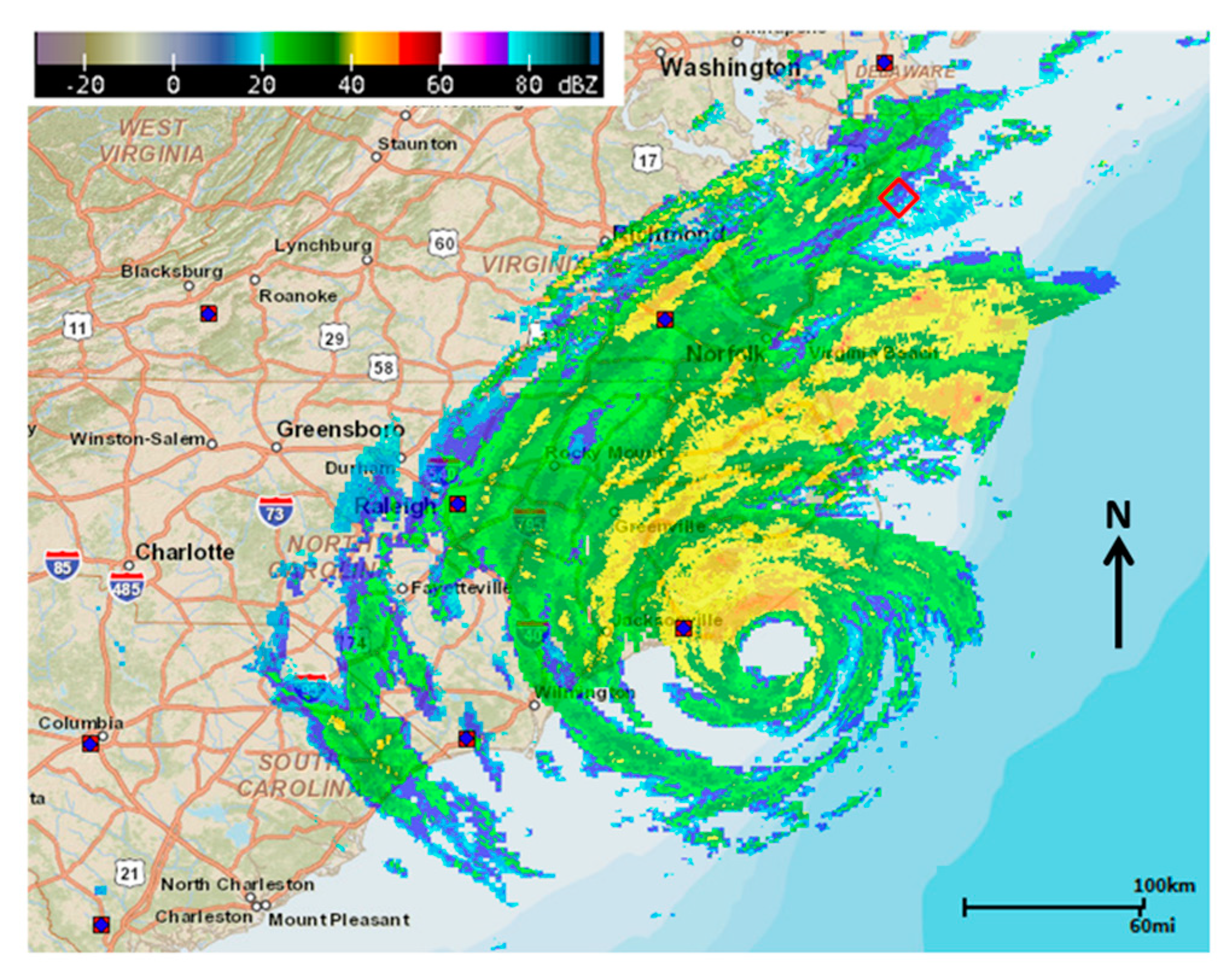
On 6 September 2019, the outer rain bands of category-1 Hurricane Dorian (henceforth Dorian) were traversing the densely instrumented NASA Precipitation Research Facility (PRF) in Wallops Island starting around 0800 and lasting to 1800 UTC. Figure 1 shows WSR-88D (Weather Service Radar-Doppler) reflectivity mosaic at 0900 UTC which depicts the location of the eyewall and rain bands about an hour before the outer bands traversed the PRF site. The eye was located about 240 km SSW of the Wallops (PRF) at this time and tracking NNE between 6 and 10 m/s. A brief analysis of the hurricane azimuthal asymmetry suggested that the shear vector was directed to the NE and the outer rain bands were located in the down shear left (DL) quadrant [46]. Several studies of hurricanes have shown that stratiform rain occurs in the DL quadrant [5,6] and typically these outer rain bands are sufficiently steady that a 1D model would be sufficient to simulate the microphysical profiles.
2.1. Surface Disdrometers and NPOL Radar
The NASA S-band polarimetric radar [47] provided excellent coverage overall, including frequent (7 min cycle) RHI (range height indicator) scans over the instrumented site (the latter is marked by a red diamond in Figure 1). The NPOL radar was located about 38 km to the north of the instrumented site. Thus, the RHI scans provided vertical slices nearly orthogonal to the outer rain band circulation direction (counter-clockwise). The NPOL is a research quality polarimetric radar that is used to provide ground validation for the spaceborne GPM (Global Precipitation Mission) rainfall algorithms and as a consequence its calibration state is carefully monitored using a variety of techniques [47,48,49]. The calibration accuracy from the latter references for ZH is to within 0.75 dB, while for ZDR it is to within 0.2 dB.
The main surface instruments were the collocated MPS and the 2DVD sited inside a double fence intercomparison reference (or DFIR), which reduces the horizontal wind speed by a factor of three relative to the ambient wind [50]. The composite drop size distribution was based on using the high resolution MPS for D < Dth and the 2DVD for D ≥ Dth where Dth is a threshold diameter in the overlap range varying from 0.75 to 1 mm [45]. Due to the high gusting winds the data quality of the MPS concentrations for D < 0.5 mm could not be established, so to be conservative we decided to use 0.5 mm as the lower limit for the MPS. Further, Dth was selected as 1 mm; thus, by combining data from two disdrometers the truncation at the small drop end was only partially overcome. The composite N(D) that resulted, while not being able to measure the drizzle mode, was considered to be a substantial improvement over using a single 2DVD alone. The MPS data processing method based on the manufacturer’s manual is described in the Appendix A of [43]; see, also, [51].
The low profile third generation 2DVD (similar to the second generation low profile described in [52]) was designed and built for NASA and has been evaluated in several studies involving intercomparisons with other disdrometers [53,54]. [Park et al.; Chang 2020]. An OTT Hydromet Pluvio weighing gage was available for measuring rain accumulations which for the rain bands was 33 mm over the entire duration (≈0800 to 1800 UTC).
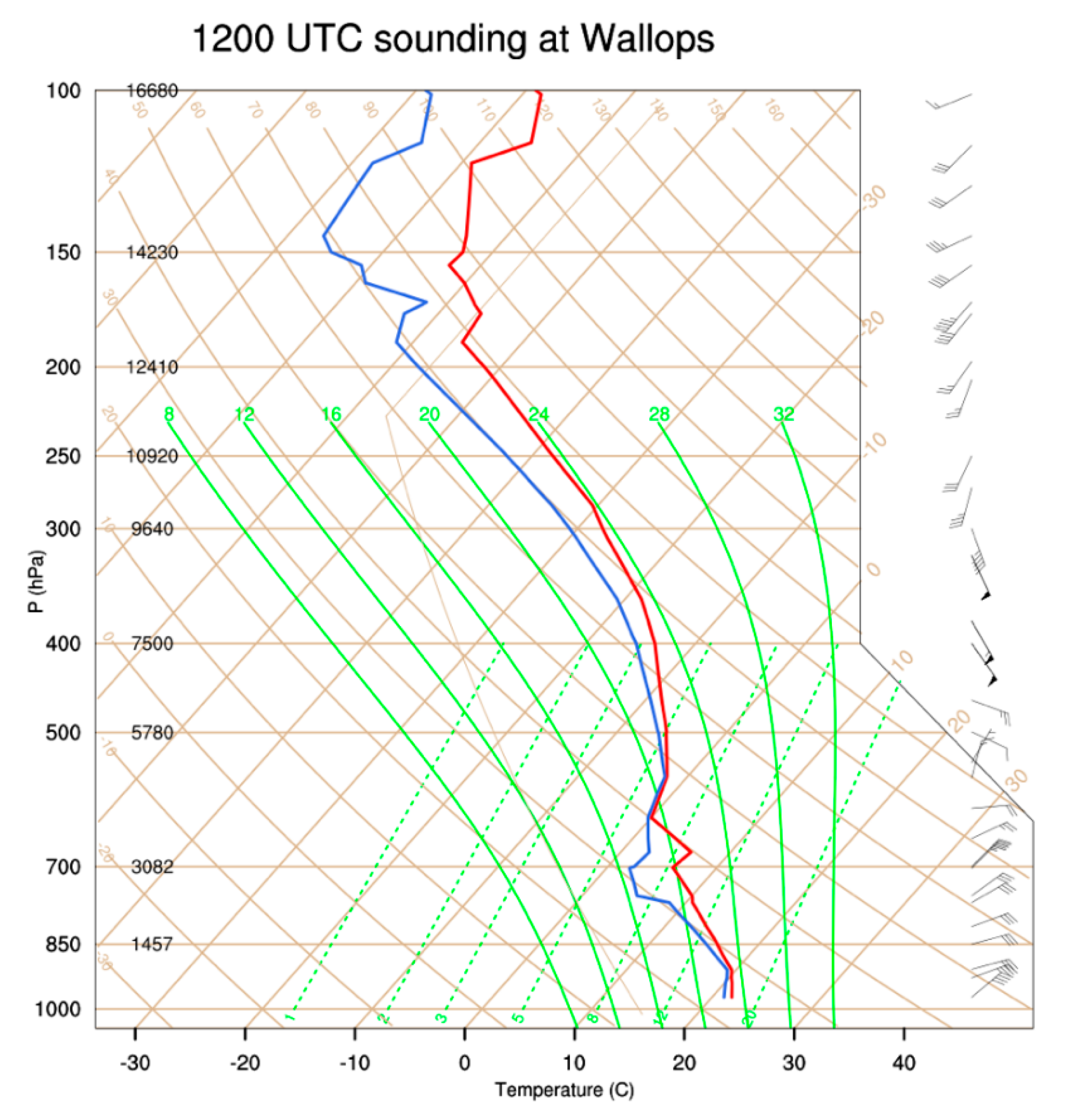
The National Weather Services’ 12 UTC sounding from Wallops Island was used in the initialization and is shown in Figure 2. Points to note are (i) the height of the 0 °C isotherm was 4.1 km, (ii) surface temperature and relative humidity (RH) were respectively, 23.6 °C and 88%, (iii) the lapse rate (from surface to 3.5 km) was −5.1 °C/km, and (iv) the RH at 0 °C was 98%. As mentioned in the Introduction, detailed analysis of the radar and disdrometer observations of the Dorian rain bands can be found in [1]. Hence, only a short overview is provided in this section along with vertical profiles of number and mass density outputs from McSnow.
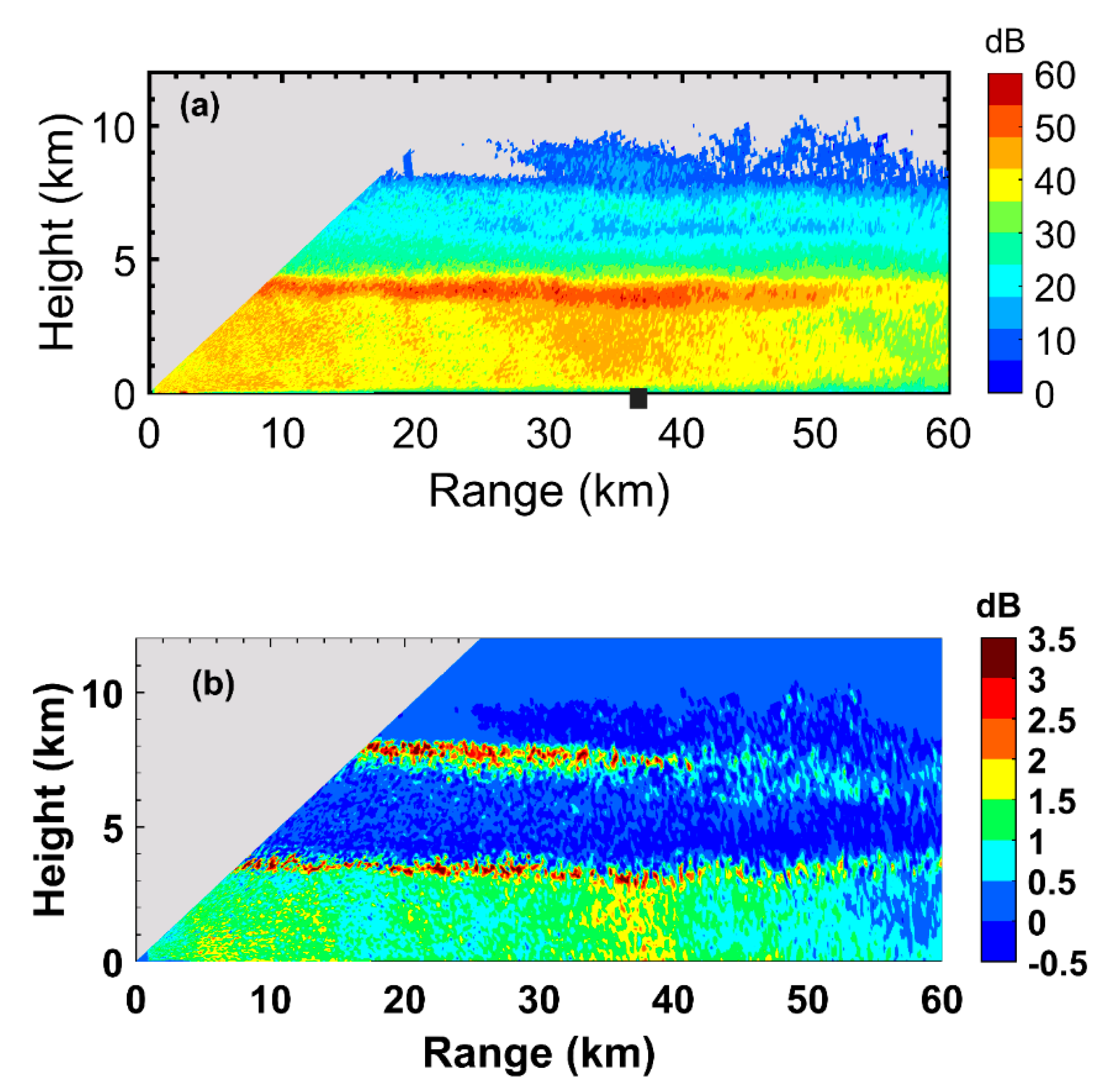
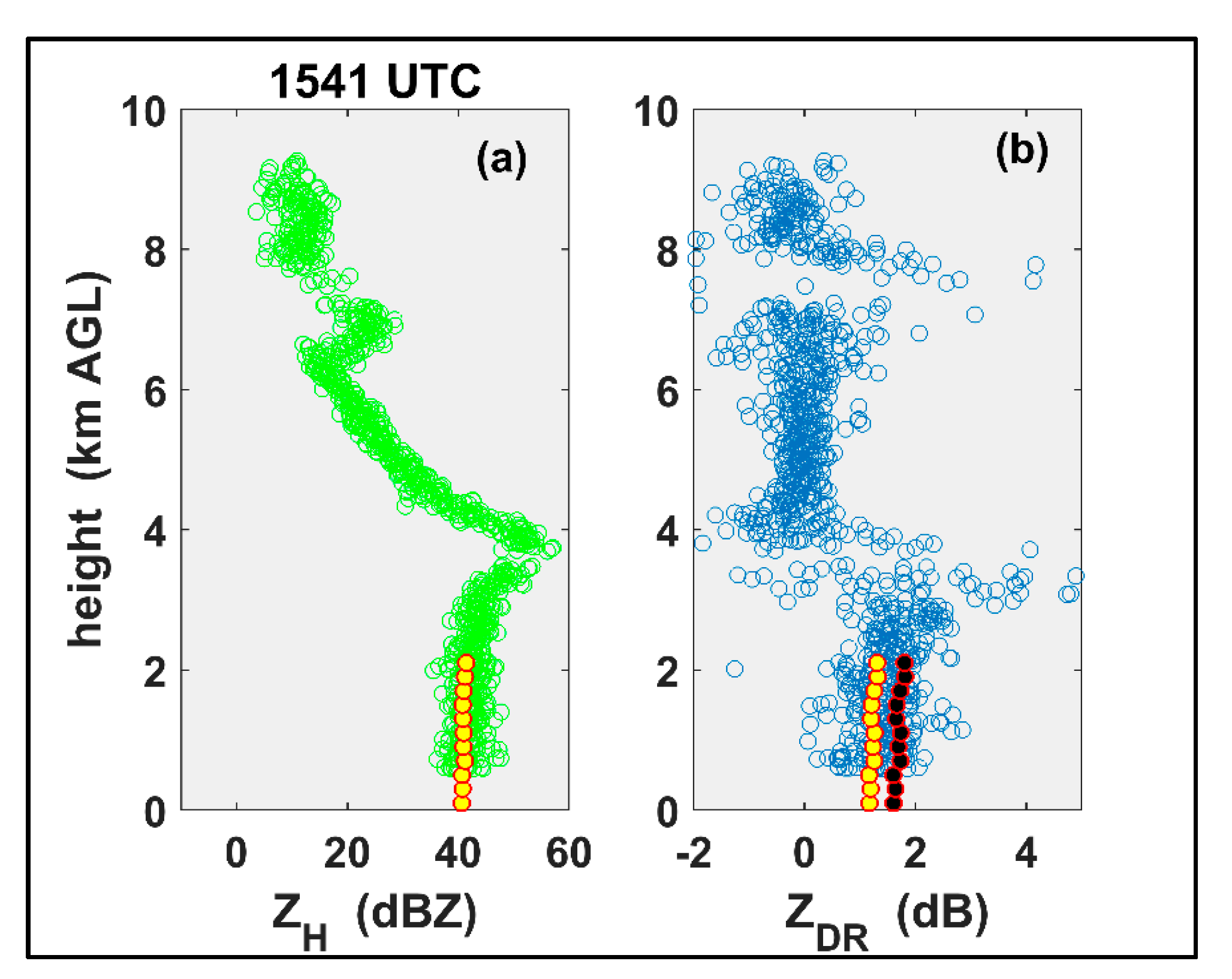
Figure 3 shows RHI scan data of (a) ZH and (b) ZDR taken at 1540 UTC along the azimuth angle to the disdrometer site (azimuth angle = 197°; marker shown at 38 km range). The intense reflectivity bright band (BB) with peak of 55 dBZ and depth of 750 m are quite unusual, along with a 12 dB drop from BB peak to lower values of 43 dBZ in the rain below. Drops larger than 5 mm were frequently recorded by the 2DVD around this and other times. In [55] it was reported that stratiform rain with thick bright band (often associated with larger melting snow particles) tend to produce larger drops, but even so, 5 mm drops (and larger) are relatively rare in non-convective events. The differential propagation phase between the radar and the site was only about 15° giving a mean specific differential phase (KDP) of 0.2 °/km. This falls in the fluctuation noise, and hence KDP values are not shown herein. Above the BB, strong aggregation can be inferred by the slope of ZH of −10 dB/km from 6.5 km height to 4.5 km (the negative slope implying increasing ZH with decreasing height due to aggregation). Riming is also likely given the very humid sounding.
The height variation of ZDR in panel (b) follows the well-known pattern of the signature of positive ZDR (≈2 to 3 dB) in the dendritic growth layer (DGL) near 7.5 km (−15 °C) [56,57] followed by a sharp drop off to 0 dB at the onset of aggregation at 7 km and continuing with no change until 4 km, where melting snow causes an increase in ZDR from 0 dB at 4 km to 2.5 dB at 3.5 km. Below 3 km to surface the ZDR varies in a narrow range about 1.5 dB characteristic of low rain rates (<10 mm/h) when combined with ZH of ≈40 dBZ.
2.2. McSnow Model
The philosophy of initializing McSnow is based on observational constraints, (a) in the DGL at the top, (b) surface rain rates at the bottom, and (c) sounding data obtained during the observations. A steady influx of ice crystals in the DGL is assumed whose ice water content (IWC) of 0.3 g/m3 is constrained by radar observed ZH ≈ 15 dBZ at 7.5 km (T = −15 °C) [58]. The number density of ice crystals is set to 200 per liter so that the mean crystal mass is around 1.5 μg. As mentioned earlier, the 12Z sounding from Wallops was suitable as it was done during the earlier rain band passages. The sounding profile thus initializes the temperature and relative humidity, which are vital for a realistic simulation that can be compared with observations.
Motivated by horizontal variability of the moisture field that cannot be measured with the soundings, we introduce an arbitrary scaling factor for the moisture profile in the model. For example, cloud liquid water that leads to riming will form in small and transient updrafts, the same is true for supersaturation over ice leading to depositional growth. This scaling factor can be tuned so that the surface rain rate from the model is close to that measured by the disdrometers. This scale factor is set at 1.035 above 2 km height for the control run. In the control run we avoid increasing the low level moisture, because this would create a low level cloud layer, and hence a seeder–feeder situation. The scale factor does lead to the presence of an additional liquid cloud layer at 600 hPa with a moderate liquid water content of 0.1 g/m3, which we find reasonable given the observed conditions.
The idealized 1D height model has 500 vertical layers, and an arbitrary box (horizontal base) area set to 5 m2. Ice supersaturation is present above 4 km height with a maximum supersaturation of 5% at 6 km height. Below 6 km the riming process (using continuous or stochastic riming options) along with aggregation occurs until melting begins when the temperature is warmer than 0 °C. The mean cloud droplet radius in the riming zone is set to 10 μm. Note that vertical profiles of temperature, humidity, and cloud water are fixed and the Lagrangian particles simulated by McSnow do neither deplete the supersaturation nor the cloud liquid water, but only grow in the prescribed environment. The fall speed follows [59] and breakup parameterizations follows [29] (see Appendix A). To reach a stationary state, we integrate the model over at least 10 h, and all statistical quantities are then averaged over the last 5 h as in [2]. The multiplicity, which is the number of real particles (RP) represented by a single super-particle (SP), is set to a relative low number of 5000 (ratio of RP/SP) to greatly reduce the simulation noise [2]. The number of SPs per grid volume is around 1000 in the DGL, drops down to 100 near the melting layer and increases in the rain below due to collisional breakup reaching again 1000 per grid volume near the surface.
The control and the numerical experiment runs are described in Table 1. The choice of the sensitivity parameters is somewhat subjective and certainly not exhaustive. Our objective is to evaluate the impact of the riming formulation (continuous versus stochastic) and the role of drop breakup on the surface DSDs. The choices in the riming algorithm have earlier been identified as a major uncertainty of McSnow [2]. A more general objective was to determine if ice microphysics aloft (i.e., at heights colder than 0 °C) had an impact on the rain below the bright band to the surface, or if a simple rainshaft model initialized at the top of the column was sufficient (as proposed in [17]).
2.3. Model Control Run and Radar Profiles
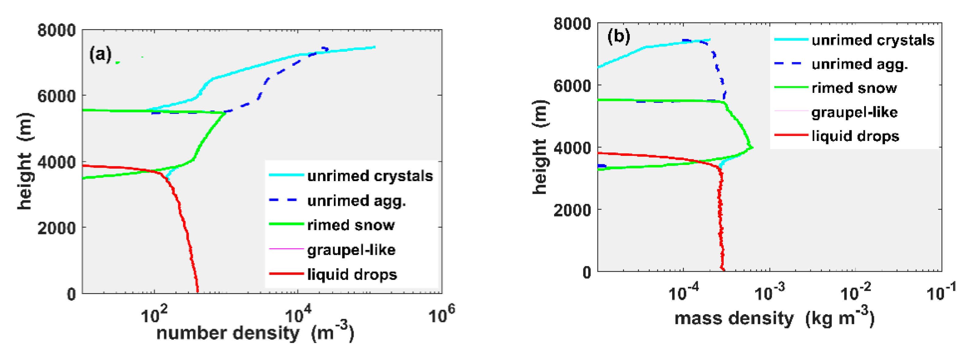
The model control run is used for vertical profiling as in Figure 4, which shows (a) number density and (b) mass density from McSnow for the listed particle types. The rapid decrease in number density from 7.5 km to near 4.5 km is due to aggregation (in the deposition/aggregation layer 5.5–8 km where supersaturation over ice is about 4–5%). The riming layer with supercooled cloud liquid starts at 6 km down to 4 km with aggregation still active to the bottom of the melting layer (i.e., aggregation of wet snow is inferred for peak ZH to reach 55 dBZ in the BB). The number density of raindrops slowly increases to the surface with a slope of about 7% (from 150 to 400 per m3 per m height from 3500 m to 0).
The mass density profile shows the peak (of 0.6 g/m3) occurring at 4.25 km (in the lower part of the mid-level liquid layer and just below the 0 °C level). The height at which the mass density of rain and rimed snow are equal occurs at 3.75 km, which is where the ZH and ZDR radar signatures clearly depict the greatest change. In the rain layer, the mass density is very steady at 0.3 g/m3. Together with the increase in the number density, it implies that the mean mass diameter should decrease with height (see Section 3).
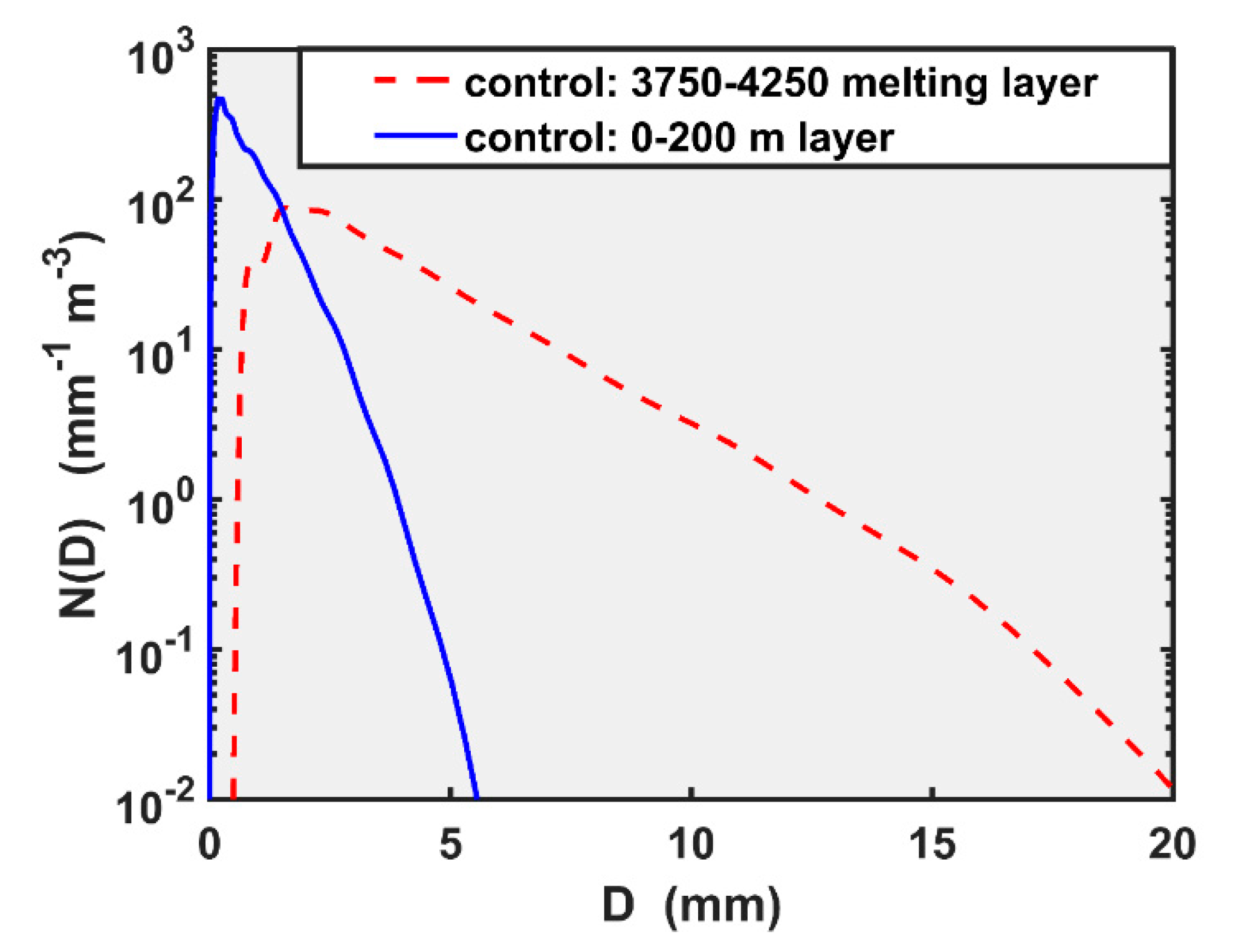
Figure 5 shows the McSnow size distributions in the lowest rain layer (0–200 m layer average) and in the layer (3.75–4.25 km) containing wet snow within bright band (BB). It is in this wet snow that polarimetric radar data (ZDR, and copolar correlation coefficient ρhv (not shown), but see Figure 6c of [1]) display prominent signatures. A polarimetric radar forward operator is currently being built to predict the signatures using the size distribution output from McSnow. Recall that McSnow can provide the size distribution conditioned on mass fraction of rime and melt water separately, which should more accurately reproduce the observed polarimetric signatures (ZDR and copolar correlation coefficient) not only in the melting level but aloft also in the DGL. Figure 5 indicates maximum sizes of wet snow can reach 20 mm in the 3.75–4.25 km layer (large enough to be in the resonance scattering regime even at S-band) with aggregation active in this layer to produce such large sizes (consistent with the unusually large 55 dBZ peak near 4 km). The Rayleigh Z computed as the sum of D6N(D) dD is 73 dBZ. For simplicity, the subscript H on Z (for horizontal polarization) is dropped until the end of this paragraph. The equivalent radar reflectivity factor (or, Ze) is given by an adjustment of Rayleigh Z by the factor {|Kice|/|Kw|}2 {ρsnow/ρice}2 where the Kice and Kw are respectively, the dielectric factors of ice and water where ρ is the density [40,60]. Since the measured Ze peak in the BB is ≈55 dBZ, the factor is inferred to be about 0.0172 or the (constant) wet snow density is ≈0.28 g/cc.
To complete the overview here, the McSnow DSDs (from the control run) in the rain from 0 to 2100 m (or 11,200-m layer averages) are used to forward model the ZH and ZDR which are then overlaid on the radar measurements. The forward model for rain used here assumes the 80-m fall “bridge” experiment drop shapes [61] and canting angle distributions (Gaussian with mean = 0 and standard deviation σβ = 7°; [62]). However, due to strong wind gusts and turbulence in hurricane rain bands we expect the drops to exhibit enhanced amplitude asymmetric oscillations on the background axisymmetric oscillation state [63,64]. Thus, the standard deviations of both axis ratios and canting angles in highly turbulent flow as in hurricane rain bands would likely not follow the still air 80-m fall bridge values. Here, we use a bulk method involving increasing (or tuning) the σβ from 7° (the still air bridge experiment value) to 20°. Note that use of 10° is common for simulating polarimetric observables from measured DSDs, which are subsequently used for developing retrieval algorithms of R without regard to the turbulent intensity [40]. Figure 6 shows the radar profiles over the disdrometer location (the scatter is due to pixel-to-pixel fluctuations as data are extracted over a number of pixels surrounding the center range 38 ± 0.5 km at heights >500 m). The overlay (yellow markers) of ZH and ZDR from McSnow DSDs with σβ tuned to 20° shows good agreement with the average radar observations (in particular the forward modeled ZDR, the ZH not being sensitive to the canting angle). Additionally shown are the ZDR values assuming σβ = 7°, which tends to be biased to larger values (relative to the radar measurements) by around 0.4 dB (see, also, Section 3).
3. Results of Control and Numerical Experiments and Comparison with Observations
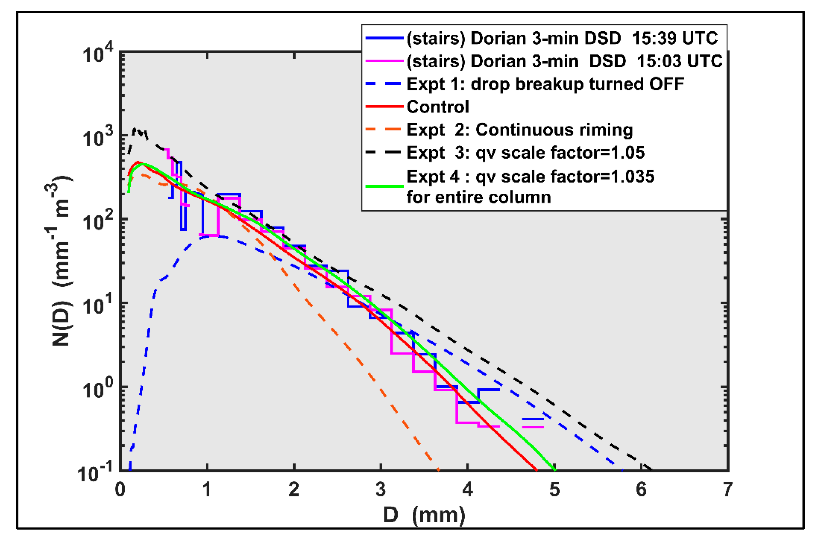
In this section the 3-min measured DSDs from the rain bands at 1503 (i.e., averaged DSDs between 1500 and 1503 period) and 1539 (1536–1539) UTC are shown in Figure 7 as a stairs plot. These DSDs are representative of the rain bands in the 1500–1600 period. The overlaid solid and dashed lines are from the control run and the four numerical experiments described in Table 1. The McSnow DSDs are an average in the 0–200 m layer in each run and as well as being averaged over the last 5 h of the simulations. Notable are the frequent occurrence of large drops, 4–6 mm, in the measured DSDs from mid-latitude outer rain bands which are generally not thought to exist in tropical/sub-tropical hurricane eyewall or (inner convective) rain bands where warm rain processes are active [8,65]. We also use the spectral width of the mass spectrum σM= {E[(D − Dm)2 D3]/M3}1/2 [66] where E stands for integration over N(D) and Dm = M4/M3 to assist with the intercomparisons.
The following points may be noted from Figure 7:
- The DSD from the control run is visually closest to the measured DSDs.
- The experiment 1 (henceforth simply, Expt. 1) where breakup is turned OFF shows severe lack of drops <1.5 mm and enhanced concentrations for D > 4 mm in accord with expectations that coalescence is active in producing large drops, but collisionally-forced breakup being turned OFF does not allow for any balance to occur.
- The DSD from Expt. 2 where continuous riming is being used forms the lower bound for concentrations for D > 2 mm and its spectral width is also the smallest (0.64 mm). This DSD gives the lowest R and ZH (shown later in Figure 8 and Figure 9). This is consistent with the notion that continuous riming leads to smaller ice particles and a narrower distribution compared to a stochastic growth equation.
- Expt. 3, where a substantial increase in the qv scale factor (Table 1) (also referred to as the area factor) to 1.05 from the control value of 1.035, shows much higher concentrations from the control DSD and much larger spectral width (1.26 mm relative to 0.9 mm for the control) leading to higher rain rates (a factor of 2 higher than the control R of 8.1 mm/h).
- Expt. 4 where the qv scale factor is same as in the control but extends through the entire column (Table 1) results in a moderate increase in surface R to 10.3 mm/h due to the presence of a lower-level liquid layer. The spectral width of this DSD (0.92 mm) is nearly equal to that of the control run and it is also close to the measured DSDs. It appears that the control run and Expt. 4 produce DSDs very close to the measured DSDs, whereas the rest of the experiments, especially 1–3, are quite a bit off.
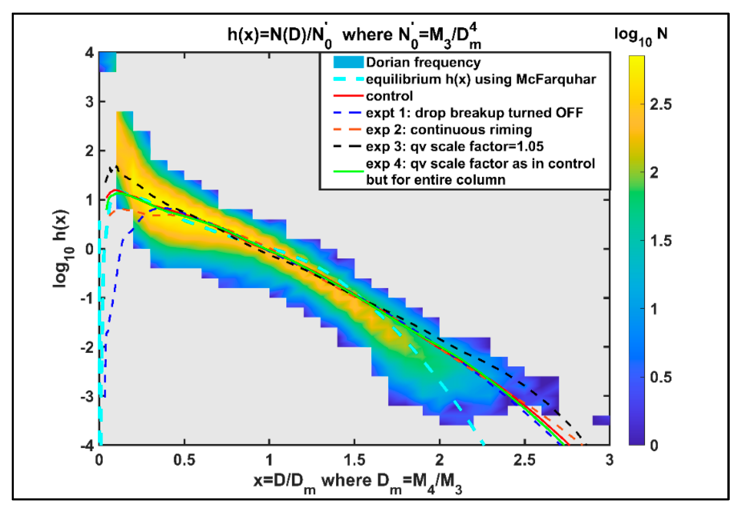
The concept of scaling-normalization [11,42] of the DSD using two reference moments (alternately, double-moment normalization) such as [M3 and M4], enables the DSD to be expressed in compact form as N(D) = N0′ h(x) where x = D/Dm, Dm = M4/M3 and N0′ = M3/Dm4. The h(x) computed from 3-min measured DSDs from all the rain bands of Dorian are shown in Figure 8 as a frequency of occurrence plot (numbers in log scale) on which are overlaid the h(x) from the McSnow control run and Expt.’s 1–4 using N(D) from the lowest layer (0–200 m). For reference, the h(x) for the equilibrium DSD (ED) from [29] (with R = 54 mm/h) as implemented in McSnow is also shown. Note that the surface measured rain rates were typically <16 mm/h and so the ED shape would not have been reached.
The following points may be noted from Figure 8:
- The control run h(x) visually passes close to the most probable h(x) (based on 3-min DSDs from the entire rain band passage) except for x > 1.8.
- The h(x) from the other experiment runs are close to the control h(x) over a broad range 0.4 < x < 2.3. This occurs due to the double moment normalization which typically reveals the underlying or intrinsic shape which for the model runs appear to be self-similar except for Expt. 1 for x < 0.4 mm.
- The model, in general, and especially Expt. 3 run (which has the highest R of 16.7 mm/h), are slow to show breakup effects in the tail; as well, there is a lack of small drops relative to the observed h(x) for x < 0.25. One should keep in mind that x is the scaled diameter so the small and large drop descriptors have to be used with caution (since Dm varies for the ED, control and the experiment runs). None of the runs have a tail (for x > 1.7) that falls faster than the ED. In fact, they more resemble an exponential fall off. The one-dimensional model of [23] has also been used in [17] who provide a detailed investigation of the effect of breakup on polarimetric radar quantities. The analysis of radar observations by [17] confirms earlier laboratory and numerical modeling results suggesting that breakup based on [26] or [29] is overaggressive and depletes large drops too quickly. However, here, we do not find any evidence that breakup is too aggressive, rather the opposite perhaps due to the moderate rain rates in this event. Recall that many large drops >5 mm were detected by the 2D-video disdrometer including one of 8 mm at 1600 UTC.
- For x < 0.25, the h(x) from the rain bands has a concave up shape and previous studies have shown that such h(x) can be fitted to the generalized gamma distribution [33,45]. The bulge in h(x) near x = 0.4 is a feature that occurs in other large databases of measured DSDs including outer bands of another hurricane Irma [33]. It may seem surprising that h(x) from the disdrometers shows the concave up shape for x < 0.25 considering the minimum D is truncated at 0.5 mm. Since x = D/Dm, it is possible for x to be as low as 0.2, for example, if minimum D is 0.5 mm and Dm is 2.5 mm. It is not clear why neither the McSnow model runs, nor the ED based h(x), show the concave up shape for x < 0.25 (except for Expt. 3). To allow for more small drops in hurricane rain bands [9] modified a tuning parameter that allowed for larger numbers of small drops to be produced by melting snow. This reduced their forward modeled ZDR to be more consistent with radar measurements in stratiform rain in hurricanes as well as in stratiform rain from MCS. A possible physical explanation would be the fragmentation of snowflakes during melting and the subsequent melting of those small ice fragments. In our case the melting layer is at a relative humidity over ice of 80–90 %, which makes melting fragmentation unlikely [67,68]. Nevertheless, such a process of snowflake-breakup is missing in McSnow and this would provide an alternative explanation for the lack of small drops below the melting layer. Adding a large number of tiny drops (<0.5 mm) whose concentrations are (say) one or two orders of magnitude larger than the control run (in Figure 7) will greatly reduce the Dmm and the ZDR while increasing R and M0 significantly. As mentioned before, the optical array probe (MPS) used herein is capable of measuring drop sizes to 0.1 mm, but the data quality in the high wind gusts could not be validated, and hence out of caution they are not shown in Figure 7.
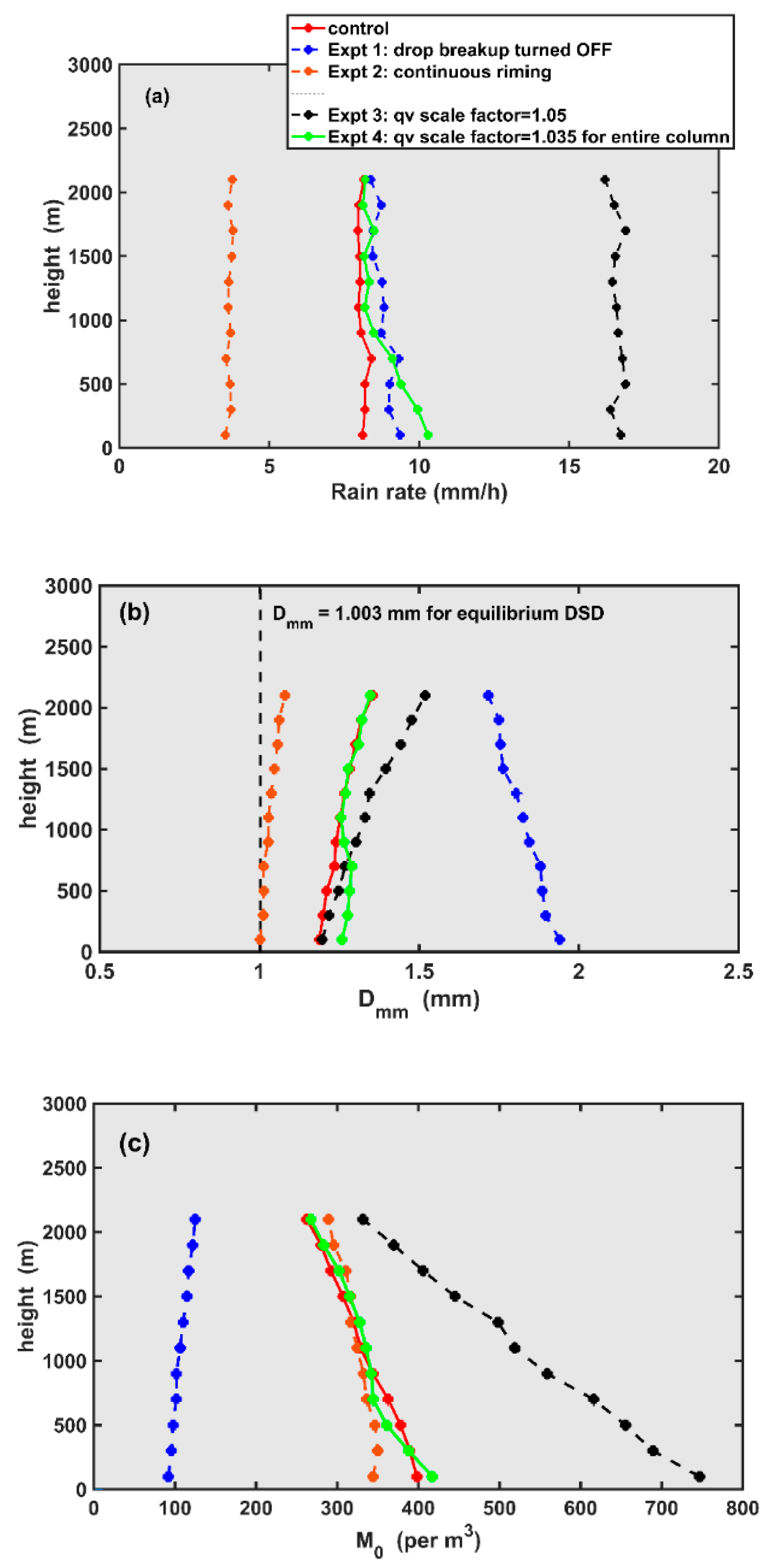
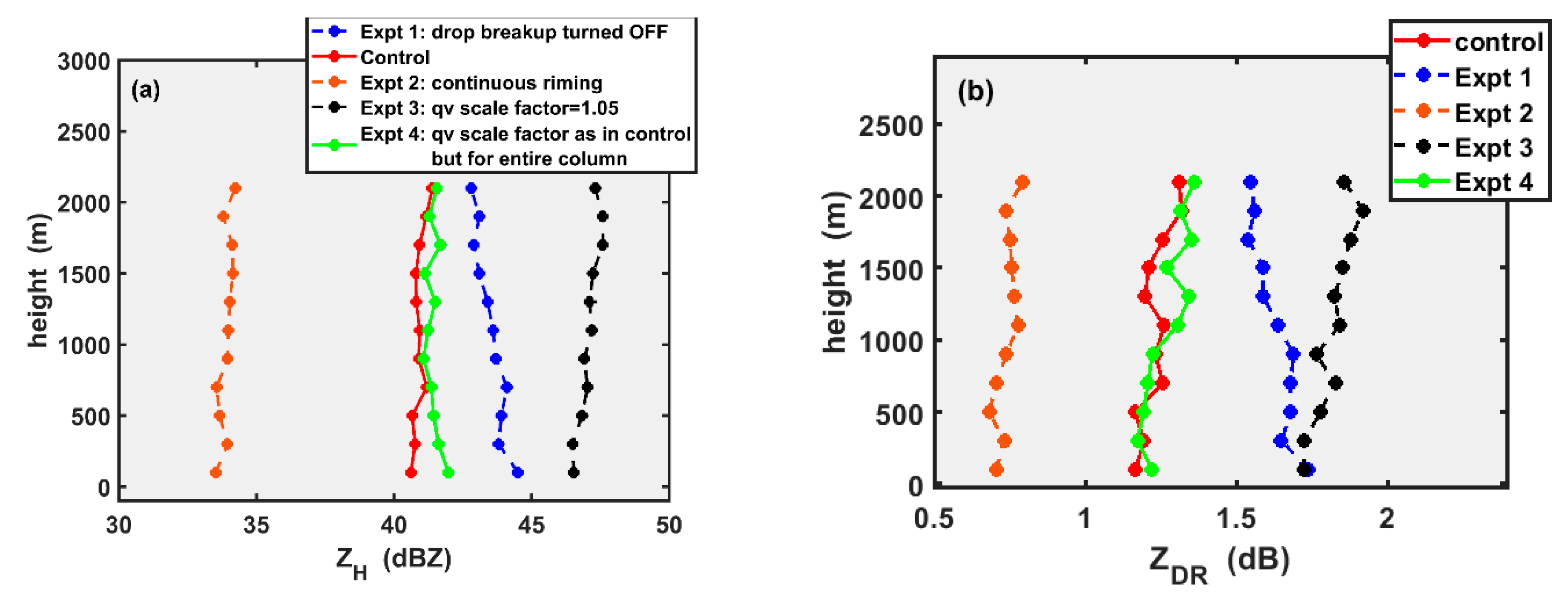
The height profiles of R, mean-mass diameter (Dmm = [M3/M0]1/3) and number density (M0 or the zeroth moment of the DSD) for heights below 2.1 km to the surface are given in Figure 9 for the control and Expt. 1–4 runs. The values are averaged in 200-m layers (total of 11 layers) and over the last 5 h of the simulations (300–600 min). Figure 10 gives the forward modeled ZH and ZDR profiles based on McSnow DSDs as input to the T-matrix scattering code (as explained earlier with reference to Figure 6).
The main assumption for calculation of ZDR (as stated in the discussion related to Figure 6) is the tuning of the standard deviation (σβ) of the canting angle to 20°as opposed to the normally used values in the range 7–10°. The σβ is used as a parameter to effectively account for mixed mode asymmetric oscillations.
The following points are made by synthesizing the information from Figure 9 and Figure 10 and relying partly on the fact that the rain rate height profile is governed approximately by the height profile of the product M0 Dmm3.5 (if evaporation and drop sorting are neglected).
- The control run shows steady R of 8.1 mm/h with a decreasing trend in Dmm from 2 km to surface (1.35 to 1.2 mm). This decrease in Dmm can be related to breakup processes. At the same time, the M0 increases from 270 m−3 at 2 km to 400 m−3 near surface. Thus, the steady R occurs due to compensating effects of the two. The ZH shows a slight tendency to decrease while ZDR decreases from 1.3 to 1.16 dB. These changes are small compared to the measurement accuracies of both ZH (to within 1 dB) and ZDR (to within 0.2 dB) but the overall trend with decreasing height could be detected by spatial averaging. The 1D rainshaft model of [17] was used to detect the fingerprint of breakup dominance if both Δ(ZH) and Δ(ZDR) < 0 (the Δ refers to difference from the top of the rainshaft to the surface). Note that ZH and ZDR depend on the higher order moments (sixth for ZH and, approximately as [M6/M3]1/3 for ZDR), so they are typically poorly correlated with Dmm or M0. While the R (8.1 mm/h) is perhaps not large enough for collisional breakup to dominate, in comparison with Expt. 1 below, the breakup in the control run is obviously an important factor in shaping the DSD to be closest to the disdrometer measurements.
- In Expt. 1, the breakup is turned OFF so the Dmm shows a large increase from 1.7 (at 2 km) to 2 mm (surface) accompanied by a small decrease in M0 from 125 to 90 m−3 as the small drops (i.e., break up fragments) are not being produced. The R shows a gradual increase from 8.3 to 9.4 mm/h at the surface which is not as large as one might expect given the Dmm3.5 amplifying factor. The model prediction of the substantial DSD shift to larger drops (see Figure 7, Expt. 1), severe lack of small drops and larger spectral width (1.2 mm) versus 0.9 mm for the control) are all consistent with coalescence as the only process. While ZH shows a trend of increasing by 2 dB with height from 2 km to surface, the ZDR also shows an overall increasing trend from 1.55 (at 2.1 km) to 1.73 dB at surface. From [17] the fingerprint of both Δ(ZH) and Δ(ZDR) > 0 (the Δ refers to difference from the top of the rainshaft to the surface) is consistent with a coalescence dominated process.
- In Expt. 2, the profile trends are somewhat similar to the control, except now both R and Dmm are at the lowest values of, respectively, 3.5 mm/h and 1 mm (the spectral width is 0.73 mm which is significantly smaller than control; obvious in Figure 7). The forward modeled ZH is also the lowest at 33 dBZ while ZDR is 0.7 dB. This suggests that the continuous riming formulation in this case is not consistent with the radar or disdrometer observations.
- In Expt. 3, a rather large increase in M0 (330 to 750 per m) and a corresponding large decrease in Dmm (1.5 to 1.1) gives the largest R at the surface of 16 mm/h. This increased R would have increased collisionally-forced breakup contributing to the Dmm decrease and M0 increase with height below 2 km to the surface. The ZH reaches its highest value of 46 dBZ, whereas ZDR does decrease a bit from 1.8 dB at 2000 m to 1.73 dB at the surface (but still the largest value compared to the other runs). This fingerprint might indicate breakup as the major process according to [17]. No doubt the increased water vapor scale-up factor, which increases from 1.035 for the control to 1.05 for Expt. 3, gives rise to these signatures but they are not in accord with the actual radar or DSD observations.
- In Expt. 4, the water vapor scale factor is same as the control except that the whole column is involved. Thus, there is increased humidity (in an already humid sounding in Figure 2) below 2 km with an additional cloud layer and consequently coalescence processes. The profiles from 2000 m to surface are nearly identical to the control run for M0, Dmm, and ZDR so the comments in (a) are relevant here also. However, below 700 m to surface the R and ZH show an increasing trend relative to control. At the surface, the R is 10.3 mm/h and ZH is 42 dBZ compared to 8.1 and 40.6 for the control, respectively. The profiles of M0, Dmm, and ZDR being nearly identical to the control run, the increase in R below 700 m to surface is a response to an increase in M0 perhaps related to increase in collisional breakup at the higher rainrate, in spite of Dmm. Here, the ΔZH below 700 m is positive, but ΔZDR < 0, so it might be indicative of both coalescence and breakup. Note from Figure 7 that the DSDs from control and Expt. 4 are nearly identical except for a slightly higher concentration of large drops > 4 mm.
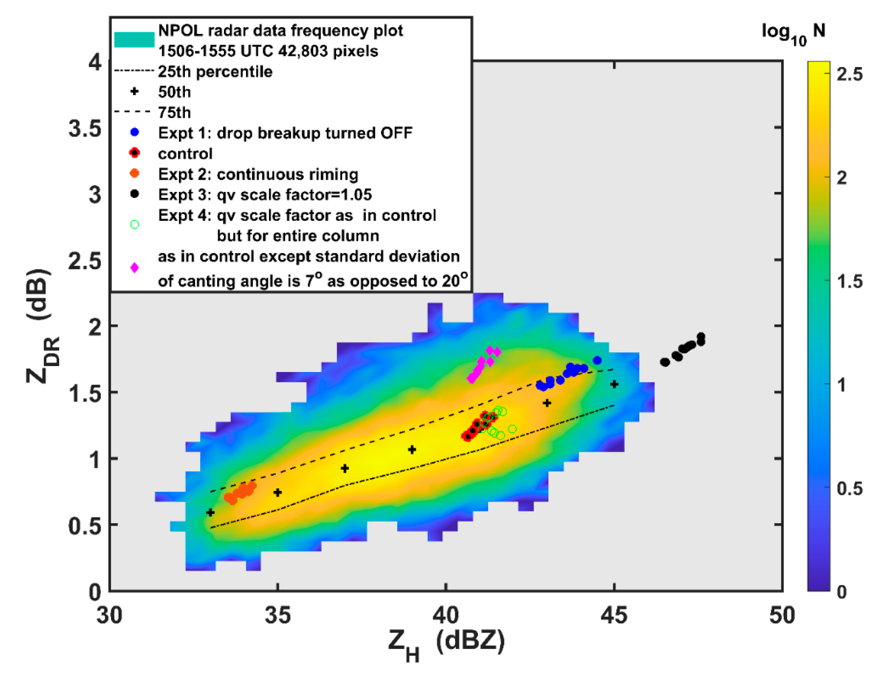
Finally, in Figure 11, we show radar data from all the RHI scans performed from 1505–1555 UTC over the instrumented site. The (ZH and ZDR) data are extracted from resolution volumes (or pixels) extending in range from 30 to 50 km, azimuth angles from 195 to 199°, and heights from 0.5 to 2 km giving a good statistical data base of nearly 43,000 points. These pairs of (ZH and ZDR) are shown as a frequency plot with the interquartile range of ZDR for each 2-dB bin width in ZH (as described in the legend). The forward modeled (ZH and ZDR) from the McSnow DSDs shown earlier in Figure 10 (from the eleven 200m-thick-layers) are overlaid on the radar frequency plot. The control run ZDR data fall close to the median. Expt. 2 (continuous riming option) and Expt. 3 (water vapor scaled up to 1.05) are obvious outliers. Expt. 1 (break up OFF) is, from Figure 7, known to have a DSD that is inconsistent with measurements, but in this higher moment space it falls in the 75th percentile though the surface value of ZH = 45 dBZ is not consistent with radar measurements. The data from Expt. 4 appears to be similar to the control run and falls close to the median and in the interquartile range except the surface ZH = 44 dB is also on the high side relative to control (42 dBZ). Excluding Expt. 4, the other runs including the control show a linear correlation between ZH and ZDR (in dB units) and the slope or dZDR/dZH is approximately the same as the slope of the median of the radar measured ZDR in 2 dB bins of ZH. Figure 11 also shows the ZDR values if the standard deviation of canting angle (σβ = 7°), which is a common assumption based on [52]. The ZDR offset from the control run with σβ = 20° is easily noted (see Figure 6c of [1]).
We now consider related issues. The inverse inference of dominant processes that control the DSD below the melting level to the surface based only on radar measurements of (ZH and ZDR) pairs is limited since the radar data are related to higher order moments or moment ratios, whereas the microphysical processes are related to lower order moments from M0 to M3+b where b is the exponent of the fall speed-D power law. There are a few articles that have attempted the retrieval of lower order moments using radar data (including specific differential phase KDP or specific attenuation, under the assumption of invariance of h(x) [69,70]). Nevertheless, the radar data as in Figure 11 have been used to advantage in detecting subtle differences between convective mid-latitude warm rain and continental rain types [71], in classification of low level (orographical induced) coalescence-dominated processes that are heavy rain producers [72], and in the recent operational application of specific attenuation for rain rate estimation where the slope of median ZDR with ZH is needed [40]. This slope from Figure 11 is estimated as close to 0.125 and using equations (10.44–10.47) of [40] the α is 0.0275 (in units of dB/°, i.e., from the relation specific attenuation = αKDP). This higher value of α (relative to 0.015 for continental rain) implies more tropical-like rain DSD characteristics of the outer rain bands of Dorian, which is not an unreasonable inference considering it is a hurricane in a maritime environment.
4. Conclusions
This case study was chosen primarily for the high quality of the radar and disdrometer observations and a representative sounding taken during the event at Wallops. The long duration (~8 h) episode of steady rainfall from the outer bands of Hurricane Dorian make this event suitable for a 1D modeling approach. The classic stratiform vertical profiles of the dendritic growth layer aloft, strong aggregation, and riming processes at altitudes from aloft to the melting level leading to a reflectivity bright band of 55 dBZ and copolar correlation minima of 0.85 in the melting layer were observed in the rain bands. The 3-min averaged rain rates, however, did not exceed 10 mm/h. The vertical profile was consistent, but the features and magnitudes did change between rain band passages across the instrumented site. Large drops were recorded by the 2D-video disdrometer with many occurrences of >5-mm sized drops and even one of 8 mm. This implies large wet snow in the melting layer (estimated to be at least resonant-sized at S-band or >15 mm).
The 1D super-particle Lagrangian model (McSnow) that simulates all the ice, melting, and rain processes in a multi-dimensional phase space was used to compare with the S-band NPOL (NASA polarimetric) radar, and with DSD measurements by collocated optical array probe and 2D-video disdrometer. The control simulation input parameters were chosen by three observational constraints involving the initialization of a steady influx of ice crystals in the radar detected dendritic growth layer at −15 °C, the availability of the National Weather Services’ sounding at Wallops during the rain band passage, and the rain rate measured by the disdrometers for the most steady period of the event.
One important issue that needed to be addressed was the unknown effects of strong wind gusts of a category-1 hurricane near the surface in disturbing the most probable shapes and orientation (canting angle) of drops deduced from the 80-m fall bridge experiments. Here, we have tuned the standard deviation of the canting angle to 20° (from the conventional assumption of 7–10°) to account effectively for multi-mode oscillations due to the strong wind gusts and turbulence. Such an adjustment brings much closer agreement between the forward modelled ZDR using DSDs from the control run and NPOL radar measurements.
Four numerical experiments (sensitivity simulations) were conducted by changing (one at a time) the important model input choices. The control run gave the best agreement with the radar profiles and the disdrometer DSDs. The vertical profiles of model DSD-derived moment and moment ratios as well as forward modeled ZH and ZDR using these same DSDs were used to infer the rain processes below 2 km to the surface. The clear outliers (based on observations) were the continuous riming formulation and turning off the breakup process. The other two outliers involved first increasing the water vapor scaling factor by 14.5% from the control, and second, keeping the water vapor scaling factor the same as in the control but applying it to the whole column. The stochastic riming model used in the control was in accord with the observations, whereas continuous riming was not. The ice microphysics above the melting layer play an important role in determining the surface DSD and R. However, while large uncertainties exist in the collision efficiency choice and droplet size used in the riming process parameterization, the control run choices were reasonably accurate in this case study.
The important role of breakup was elucidated by comparing the experiment of turning off breakup process with the control. We have shown that collisional breakup plays an important role in shaping the raindrop size distribution even at a moderate rain rate of ~10 mm/h. It is recognized that parameterization of the distribution of drop fragments following the more energetic collisions between mm-sized larger drops with sub-millimeter (≈0.5 mm) sized drops has a large uncertainty and numerical convergence issues [26,29,30]. Among these uncertainties are algorithmic choices, like the method to ensure mass conservation in collisional breakup or the uncertainty in the type of breakup (see Appendix A). The Monte-Carlo simulation of collisional breakup has in principle some advantages over the more common bin microphysics, but for the super-droplet model presented here we find a lack of a filament peak. This filament peak is more pronounced in earlier studies using bin microphysics. Clearly some of these issues can be resolved by careful wind tunnel studies as in [39] and are much needed to reconcile the different numerical approaches to determining the shape of the equilibrium distribution prior to confident application to non-equilibrium rain rate simulations.
An alternative explanation for the lack of small raindrops below the melting layer would be melting fragmentation, i.e., the breakup of snowflakes during melting, as it is described for example in [67,68]. A quantitative parameterization of melting fragmentation might even be more challenging than the long-standing breakup problem of raindrops.
Author Contributions
Conceptualization, V.B., A.S., and W.W.; methodology, A.S., V.B., W.W., M.T., and G.-J.H.; McSnow algorithm, A.S. and C.S. developed McSnow and implemented the new Monte-Carlo algorithm for collisional breakup; writing—original draft preparation, V.B.; and writing—review and editing, V.B., A.S., W.W., and C.S. All authors have read and agreed to the published version of the manuscript.
Funding
This research was funded by the National Science Foundation, grant number AGS-1901585 to Colorado State University (V.B., M.T.). Deutscher Wetterdienst (A.S. and C.S.) received funding from the German Science Foundation (DFG) under grant SE 1784/3-1, project ID 408011764 as part of the DFG priority program SPP 2115 on radar polarimetry.
Acknowledgments
V.N.B. acknowledges useful discussion with Michael Bell and Patrick Kennedy at Colorado State University. NPOL radar data was made available by David Wolff and David Marks of NASA Precipitation Research Facility at Wallops, Virginia, USA.
Conflicts of Interest
The authors declare no conflict of interest. The funders had no role in the design of this study; in the collection, analyses, or interpretation of its data; in the writing of this manuscript, and in the decision to publish these results.
Appendix A. Implementation of Collisional Breakup in the Super-Droplet Method
The Monte-Carlo super-droplet method described in [3] provides an efficient algorithm to solve the kinetic collection equation (KCE) describing collision-coalescence of cloud droplets and raindrops. A unique feature that distinguishes this approach from other Monte-Carlo solvers of the KCE is that the number of simulated Lagrangian particles (also known as super-droplets) is constant during collision-coalescence. This is ensured by predicting additional weights, called the multiplicity of super-droplets, which correspond to the ratio of super-droplets to real drops. Collisional breakup creates additional droplets that can be very different in size from the remnants of the original drops after the breakup event. Hence, an implementation that conserves the number of super-droplets seems impossible. If we accept that new super-droplets are created by a breakup event, the implementation of collisional breakup in the super-droplet framework becomes straightforward, especially when using the fragment distributions as given in [29]. For each super-droplet collision event we determine the coalescence and breakup probability, the breakup mode, and the number of fragments using the parameterizations of [26] and [73] detailed in [28].
For filament breakup we draw one drop (diameter) from
where and are the mean and the standard deviation of a log-normal distribution and are given by Equations (17) and (18) of [29], and is a normally distributed random number. For the 2nd mode we draw another drop from
where and are the mean and the standard deviation of a normal distribution as given by Equations (19) and (20) of [29], and is another normally distributed random number. The third drop mode is then given by mass conservation. For sheet and disk breakup we proceed accordingly but only two drop modes remain, because the remnant of the smaller original drop cannot be distinguished from the fragments. Hence, we draw only one drop (diameter) from Equations (21) and (22) of [29] in case of sheet or from Equations (24) and (25) in case of disk breakup. The remnant of the large drop, which defines the second mode, is again given by mass conservation. Hence, only filament breakup creates one new super-droplet per breakup event. The multiplicity of each super-droplet after the breakup event follows directly from the number of drops in each breakup mode. In contrast to a bin microphysical implementation, the mass conservation is thus ensured for each individual super-droplet collision and not only as an integral constraint on the drop distribution. This also explains why not all equations of [29] are needed for the super-droplet implementation. For example, the assumption of a Gaussian distribution for the remnant of the large drop is not necessary, instead the fragment distribution of the large drop is a direct result of mass conservation of the individual collisions. However, for some rare breakup events it can happen that the drops drawn from the fragment distributions of the small drops already exceed the combined mass of the original drops. For simplicity we reject those rare mass-violating breakup events and allow coalescence for those collisions. Alternatively, one could draw again from the fragment distribution.
References
- Thurai, M.; Bringi, V.N.; Wolff, D.B.; Marks, D.; Pabla, C.S. Drop size distribution measurements in outer rainbands of hurricane dorian at the NASA wallops precipitation-research facility. Atmosphere 2020, 11, 578. [Google Scholar] [CrossRef]
- Brdar, S.; Seifert, A. McSnow: A monte-carlo particle model for riming and aggregation of ice particles in a multidimensional microphysical phase space. J. Adv. Model. Earth Syst. 2018, 10, 187–206. [Google Scholar] [CrossRef] [Green Version]
- Shima, S.; Kusano, K.; Kawano, T.; Sugiyama, T.; Kawahara, S. The super-droplet method for the numerical simulation of clouds and precipitation: A particle-based and probabilistic microphysics model coupled with a non-hydrostatic model. Q. J. R. Meteorol. Soc. 2009, 135, 1307–1320. [Google Scholar] [CrossRef] [Green Version]
- Feng, Y.-C.; Bell, M. Microphysical characteristics of an asymmetric eyewall in major Hurricane Harvey. Geophys. Res. Lett. 2019, 46, 461–471. [Google Scholar] [CrossRef] [Green Version]
- Didlake, A.C.; Kumjian, M.R. Examining storm asymmetries in Hurricane Irma (2017) using polarimetric radar observations. Geophys. Res. Lett. 2018, 45, 13513–13522. [Google Scholar] [CrossRef]
- Didlake, A.C.; Kumjian, M.R. Examining polarimetric radar observations of bulk microphysical structures and their relation to vortex kinematics in hurricane arthur (2014). Mon. Weather Rev. 2017, 145, 4521–4541. [Google Scholar] [CrossRef]
- Wang, M.; Zhao, K.; Lee, W.-C.; Zhang, F. Microphysical and kinematic structure of convective-scale elements in the inner rainband of Typhoon Matmo (2014) after landfall. J. Geophys. Res. Atmos. 2018, 123, 6549–6564. [Google Scholar] [CrossRef] [Green Version]
- Brown, B.R.; Bell, M.M.; Frambach, A.J. Validation of simulated hurricane drop size distributions using polarimetric radar. Geophys. Res. Lett. 2016, 43, 910–917. [Google Scholar] [CrossRef]
- Brown, B.R.; Bell, M.M.; Thompson, G. Improvements to the snow melting process in a partially double moment microphysics parameterization. J. Adv. Model. Earth Syst. 2017, 9, 1150–1166. [Google Scholar] [CrossRef] [Green Version]
- Wang, M.; Zhao, K.; Pan, Y.; Xue, M. Evaluation of simulated drop size distributions and microphysical processes using polarimetric radar observations for landfalling Typhoon Matmo (2014). J. Geophys. Res. Atmos. 2020, 125. [Google Scholar] [CrossRef]
- Testud, J.; Oury, S.; Black, R.A.; Amayenc, P.; Dou, X. The concept of “Normalized” distribution to describe raindrop spectra: A tool for cloud physics and cloud remote sensing. J. Appl. Meteorol. 2001, 40, 1118–1140. [Google Scholar] [CrossRef]
- Bringi, V.N.; Chandrasekar, V.; Hubbert, J.; Gorgucci, E.; Randeu, W.L.; Schoenhuber, M. Raindrop size distribution in different climatic regimes from disdrometer and dual-polarized radar analysis. J. Atmos. Sci. 2003, 60, 354–365. [Google Scholar] [CrossRef]
- Kennedy, P.C.; Rutledge, S.A. S-band dual-polarization radar observations of winter storms. J. Appl. Meteorol. Climatol. 2011, 50, 844–858. [Google Scholar] [CrossRef]
- Schrom, R.S.; Kumjian, M.R.; Lu, Y. Polarimetric radar signatures of dendritic growth zones within Colorado winter storms. J. Appl. Meteorol. Climatol. 2005, 54, 2365–2388. [Google Scholar] [CrossRef]
- Moisseev, D.N.; Lautaportti, S.; Tyynela, J.; Lim, S. Dual-polarization radar signatures in snowstorms: Role of snowflake aggregation. J. Geophys. Res. Atmos. 2015, 120, 12644–12655. [Google Scholar] [CrossRef] [Green Version]
- Trömel, S.; Ryzhkov, A.V.; Hickman, B.; Mühlbauer, K.; Simmer, C. Polarimetric radar variables in the layers of melting and dendritic growth at X band—Implications for a nowcasting strategy in stratiform rain. J. Appl. Meteorol. Climatol. 2019, 58, 2497–2522. [Google Scholar] [CrossRef]
- Kumjian, M.R.; Prat, O.P. The impact of raindrop collisional processes on the polarimetric radar variables. J. Atmos. Sci. 2014, 71, 3052–3067. [Google Scholar] [CrossRef]
- Rasmussen, R.M.; Heymsfield, A.J. Melting and shedding of graupel and hail. Part I: Model physics. J. Atmos. Sci. 1987, 44, 2754–2763. [Google Scholar] [CrossRef] [Green Version]
- Bringi, V.N.; Rasmussen, R.M.; Vivekanandan, J. Multiparameter radar measurements in Colorado Convective Storms. Part I: Graupel melting studies. J. Atmos. Sci. 1986, 43, 2545–2563. [Google Scholar] [CrossRef] [Green Version]
- Kumjian, M.R.; Ganson, S.M.; Ryzhkov, A.V. Freezing of raindrops in deep convective updrafts: A microphysical and polarimetric model. J. Atmos. Sci. 2012, 69, 3471–3490. [Google Scholar] [CrossRef]
- Hu, Z.; Srivastava, R.C. Evolution of raindrop size distribution by coalescence, breakup, and evaporation: Theory and observations. J. Atmos. Sci. 1995, 52, 1761–1783. [Google Scholar] [CrossRef] [Green Version]
- Prat, O.P.; Barros, A.P. A robust numerical solution of the stochastic collection–breakup equation for warm rain. J. Appl. Meteorol. Climatol. 2007, 46, 1480–1497. [Google Scholar] [CrossRef] [Green Version]
- Prat, O.P.; Barros, A.P.; Williams, C.R. an intercomparison of model simulations and VPR estimates of the vertical structure of warm stratiform rainfall during TWP-ICE. J. Appl. Meteorol. Climatol. 2008, 47, 2797–2815. [Google Scholar] [CrossRef]
- Barthes, L.; Mallet, C. Vertical evolution of raindrop size distribution: Impact on the shape of the DSD. Atmos. Res. 2013, 119, 13–22. [Google Scholar] [CrossRef]
- Brazier-Smith, P.; Jennings, R.; Latham, S.G.; Mason, J.; John, B. The interaction of falling water drops: Coalescence. Proc. R. Soc. Lond. 1997, A326, 393–408. [Google Scholar] [CrossRef]
- Low, T.B.; List, R. Collision, coalescence and breakup of raindrops. Part II: Parameterization of fragment size distributions. J. Atmos. Sci. 1982, 39, 1607–1619. [Google Scholar] [CrossRef]
- Arabas, S.; Shima, S. Large-eddy simulations of trade wind cumuli using particle-based microphysics with monte carlo coalescence. J. Atmos. Sci. 2013, 70, 2768–2777. [Google Scholar] [CrossRef] [Green Version]
- Seifert, A.; Khain, A.; Blahak, U.; Beheng, K.D. Possible effects of collisional breakup on mixed-phase deep convection simulated by a spectral (Bin) cloud model. J. Atmos. Sci. 2005, 62, 1917–1931. [Google Scholar] [CrossRef]
- McFarquhar, G.M. A new representation of collision-induced breakup of raindrops and its implications for the shapes of raindrop size distributions. J. Atmos. Sci. 2004, 61, 777–794. [Google Scholar] [CrossRef] [Green Version]
- Straub, W.; Beheng, K.D.; Seifert, A.J.; Schlottke, J.; Weigand, B. Numerical investigation of collision-induced breakup of raindrops. Part II: Parameterizations of coalescence efficiencies and fragment size distributions. J. Atmos. Sci. 2010, 67, 576–588. [Google Scholar] [CrossRef] [Green Version]
- D’Adderio, L.; Porcù, F.; Tokay, A. Identification and analysis of collisional breakup in natural rain. J. Atmos. Sci. 2015, 72, 3404–3416. [Google Scholar] [CrossRef]
- D’Adderio, L.; Porcù, F.; Tokay, A. Evolution of drop size distribution in natural rain. Atmos. Res. 2018, 200, 70–76. [Google Scholar] [CrossRef]
- Zawadzki, I.; Antonio, M.D.A. Equilibrium raindrop size distributions in tropical rain. J. Atmos. Sci. 1988, 45, 3452–3459. [Google Scholar] [CrossRef] [Green Version]
- Jacobson, M.Z. Numerical solution to drop coalescence/breakup with a volume-conserving, positive-definite, and unconditionally stable scheme. J. Atmos. Sci. 2011, 68, 334–346. [Google Scholar] [CrossRef] [Green Version]
- Verlinde, J.; Flatau, P.J.; Cotton, W.R. Analytical solutions to the collection growth equation: Comparison with approximate methods and application to cloud microphysics parameterization schemes. J. Atmos. Sci. 1990, 47, 2871–2880. [Google Scholar] [CrossRef] [Green Version]
- Seifert, A.; Beheng, K. A two-moment cloud microphysics parameterization for mixed-phase clouds. Part 1: Model description. Meteorol. Atmos. Phys. 2006, 92, 45–66. [Google Scholar] [CrossRef]
- Morrison, H.; Tessendorf, S.A.; Ikeda, K.; Thompson, G. Sensitivity of a simulated midlatitude squall line to parameterization of raindrop breakup. Mon. Weather Rev. 2012, 140, 2437–2460. [Google Scholar] [CrossRef] [Green Version]
- Paukert, M.; Fan, J.; Rasch, P.J.; Morrison, H.; Milbrandt, J.A.; Shpund, J.; Khain, A. Three-moment representation of rain in a bulk microphysics model. J. Adv. Model. Earth Syst. 2019, 11, 257–277. [Google Scholar] [CrossRef] [Green Version]
- Szakáll, M.; Urbich, I. Wind tunnel study on the size distribution of droplets after collision induced breakup of levitating water drops. Atmos. Res. 2018, 213, 51–56. [Google Scholar] [CrossRef]
- Ryzhkov, A.V.; Zrnic, D.S. Radar Polarimetry for Weather Observations; Springer Nature: Cham, Switzerland, 2019. [Google Scholar]
- Kumjian, M.R.; Lebo, Z.J.; Morrison, H.C. On the mechanisms of rain formation in an idealized supercell storm. Mon. Weather Rev. 2015, 143, 2754–2773. [Google Scholar] [CrossRef] [Green Version]
- Lee, G.W.; Zawadzki, I.; Szyrmer, W.; Sempere-Torres, D.; Uijlenhoet, R. A General approach to double-moment normalization of drop size distributions. J. Appl. Meteorol. 2004, 43, 264–281. [Google Scholar] [CrossRef] [Green Version]
- Thurai, M.; Gatlin, P.; Bringi, V.N.; Petersen, W.; Kennedy, P.; Notaroš, B.; Carey, L. Toward completing the raindrop size spectrum: Case studies involving 2D-Video disdrometer, droplet spectrometer, and polarimetric radar measurements. J. Appl. Meteorol. Climatol. 2017, 56, 877–896. [Google Scholar] [CrossRef]
- Thurai, M.; Bringi, V.N. Application of the generalized gamma model to represent the full rain drop size distribution spectra. J. Appl. Meteorol. Climatol. 2018, 57, 1197–1210. [Google Scholar] [CrossRef]
- Raupach, T.H.; Thurai, M.; Bringi, V.N.; Berne, A. Reconstructing the drizzle mode of the raindrop size distribution using double-moment normalization. J. Appl. Meteorol. Climatol. 2019, 58, 145–164. [Google Scholar] [CrossRef]
- DeHart, J.C.; Bell, M.M. A comparison of the polarimetric radar characteristics of heavy rainfall from Hurricanes Harvey (2017) and Florence (2018). J. Geophys. Res. Atmos. 2020, 125. [Google Scholar] [CrossRef]
- Wolff, D.B.; Marks, D.A.; Petersen, W.A. General application of the Relative Calibration Adjustment (RCA) technique for monitoring and correcting radar reflectivity calibration. J. Atmos. Ocean. Technol. 2015, 32, 496–506. [Google Scholar] [CrossRef]
- Silberstein, D.S.; Wolff, D.B.; Marks, D.; Atlas, D.; Pippitt, J.L. Ground clutter as a monitor of radar stability at Kwajalein, RMI. J. Atmos. Ocean. Technol. 2008, 25, 2037–2045. [Google Scholar] [CrossRef]
- Hunzinger, A.; Hardin, J.; Bharadwaj, N.; Varble, A.; Matthews, A. An extended radar relative calibration adjustment (eRCA) technique for higher-frequency radars and range–height indicator (RHI) scans. Atmos. Meas. Tech. 2020, 13, 3147–3166. [Google Scholar] [CrossRef]
- Notaroš, B.M.; Bringi, V.N.; Kleinkort, C.; Kennedy, P.; Huang, G.-J.; Thurai, M.; Newman, A.J.; Bang, W.; Lee, G. Accurate characterization of winter precipitation using multi-angle snowflake camera, visual hull, advanced scattering methods and polarimetric radar. Atmosphere 2016, 7, 81. [Google Scholar] [CrossRef] [Green Version]
- Baumgardner, D.; Kok, G.; Dawson, W.; O’Connor, D.; Newton, R. A new ground-based precipitation spectrometer: The Meteorological Particle Sensor (MPS). In Proceedings of the 11th Conference on Cloud Physics, Ogden, UT, USA, 3–7 June 2002; p. 8. [Google Scholar]
- Schönhuber, M.; Lammer, G.; Randeu, W.L. The 2D-Video-Disdrometer. Precipitation: Advances in Measurement, Estimation and Prediction; Michaelides, S.C., Ed.; Springer: New York, NY, USA, 2008; pp. 3–31. [Google Scholar]
- Park, S.; Kim, H.; Ham, Y.; Jung, S. Comparative evaluation of the OTT PARSIVEL2 using a collocated two-dimensional video disdrometer. J. Atmos. Ocean. Technol. 2017, 34, 2059–2082. [Google Scholar] [CrossRef]
- Chang, W.-Y.; Lee, G.; Jou, B.-D.; Lee, W.-C.; Lin, P.-L.; Yu, C.-K. Uncertainty in measured raindrop size distributions from four types of collocated instruments. Remote Sens. 2020, 12, 1167. [Google Scholar] [CrossRef] [Green Version]
- Gatlin, P.N.; Petersen, W.A.; Knupp, K.R.; Carey, L.D. Observed response of the raindrop size distribution to changes in the melting layer. Atmosphere 2018, 9, 319. [Google Scholar] [CrossRef] [Green Version]
- Bechini, R.; Baldini, L.; Chandrasekar, V. Polarimetric radar observations in the ice region of precipitating clouds at C-band and X-band radar frequencies. J. Appl. Meteorol. Climatol. 2013, 52, 1147–1169. [Google Scholar] [CrossRef]
- Griffin, E.; Schuur, T.; Ryzhkov, A. A polarimetric analysis of ice microphysical processes in snow, using quasi-vertical profiles. J. Appl. Meteorol. Climatol. 2018, 57, 31–50. [Google Scholar] [CrossRef]
- Hogan, R.J.; Mittermaier, M.P.; Illingworth, A.J. The retrieval of ice water content from radar reflectivity factor and temperature and its use in evaluating a mesoscale model. J. Appl. Meteorol. Climatol. 2006, 45, 301–317. [Google Scholar] [CrossRef] [Green Version]
- Khvorostyanov, V.I.; Curry, J.A. Fall velocities of hydrometeors in the atmosphere: Refinements to a continuous analytical power law. J. Atmos. Sci. 2005, 62, 4343–4357. [Google Scholar] [CrossRef]
- Bringi, V.N.; Chandrasekar, V. Polarimetric Doppler Weather Radar: Principles and Applications; Cambridge University Press: Cambridge, UK, 2001; p. 636. [Google Scholar]
- Thurai, M.; Huang, G.-J.; Bringi, V.N.; Randeu, W.L.; Schönhuber, M. Drop shapes, model comparisons, and calculations of polarimetric radar parameters in rain. J. Atmos. Ocean. Technol. 2007, 24, 1019–1032. [Google Scholar] [CrossRef]
- Huang, G.; Bringi, V.N.; Thurai, M. Orientation angle distributions of drops after an 80-m fall using a 2D video disdrometer. J. Atmos. Ocean. Technol. 2008, 25, 1717–1723. [Google Scholar] [CrossRef]
- Thurai, M.; Bringi, V.N.; Szakáll, M.; Mitra, S.K.; Beard, K.V.; Borrmann, S. Drop shapes and axis ratio distributions: Comparison between 2D video disdrometer and wind-tunnel measurements. J. Atmos. Ocean. Technol. 2009, 26, 1427–1432. [Google Scholar] [CrossRef]
- Szakáll, M.; Diehl, K.; Mitra, S.K.; Borrmann, S. A wind tunnel study on the shape, oscillation, and internal circulation of large raindrops with sizes between 2.5 and 7.5 mm. J. Atmos. Sci. 2009, 66, 755–765. [Google Scholar] [CrossRef]
- Wang, M.; Zhao, K.; Xue, M.; Zhang, G.; Liu, S.; Wen, L.; Chen, G. Precipitation microphysics characteristics of a Typhoon Matmo (2014) rainband after landfall over eastern China based on polarimetric radar observations. J. Geophys. Res. Atmos. 2016, 121, 12415–12433. [Google Scholar] [CrossRef]
- Haddad, Z.S.; Durden, S.L.; Im, E. Parameterizing the raindrop size distribution. J. Appl. Meteorol. 1996, 35, 3–13. [Google Scholar] [CrossRef] [Green Version]
- Oraltay, R.G.; Hallett, J. Evaporation and melting of ice crystals: A laboratory study. Atmos. Res. 1989, 24, 169–189. [Google Scholar] [CrossRef]
- Oraltay, R.G.; Hallett, J. The melting layer: A laboratory investigation of ice particle melt and evaporation near 0 C. J. Appl. Meteorol. 2005, 44, 206–220. [Google Scholar] [CrossRef]
- Raupach, T.H.; Berne, A. Retrieval of the raindrop size distribution from polarimetric radar data using double-moment normalization. Atmos. Meas. Tech. 2017, 10, 2573–2594. [Google Scholar] [CrossRef] [Green Version]
- Bringi, V.; Mishra, K.V.; Thurai, M.; Kennedy, P.C.; Raupach, T.H. Retrieval of lower-order moments of the drop size distribution using CSU-CHILL X-band polarimetric radar: A case study. Atmos. Meas. Tech. 2020. in review. [Google Scholar] [CrossRef]
- Carr, N.; Kirstetter, P.; Gourley, J.; Hong, Y. Polarimetric Signatures of midlatitude warm-rain precipitation events. J. Appl. Meteorol. Climatol. 2017, 56, 697–711. [Google Scholar] [CrossRef]
- Porcacchia, L.; Kirstetter, P.E.; Gourley, J.J.; Maggioni, V.; Cheong, B.L.; Anagnostou, M.N. Toward a polarimetric radar classification scheme for coalescence-dominant precipitation: Application to complex terrain. J. Hydrometeorol. 2017, 18, 3199–3215. [Google Scholar] [CrossRef]
- Beard, K.V.; Ochs, H.T. Collisions between small precipitation drops. Part II: Formulas for coalescence, temporary coalescence, and satellites. J. Atmos. Sci. 1995, 52, 3977–3996. [Google Scholar] [CrossRef] [Green Version]
Figure 1.
Mosaic of reflectivity from the WSR-88D radars of Hurricane Dorian at 0900 UTC on 16 September 2019. The red diamond marker is the location of the surface instrumented site at NASA’s Precipitation Research Facility (PRF). The NPOL radar operated by NASA is 38 km north of the NASA Precipitation Research Facility (PRF).

Figure 2.
The 12 UTC sounding from Wallops on 16 September 2019.

Figure 3.
NPOL radar range height indicator (RHI) scan along the 197° azimuth angle; the black square marker locates the instrumented site. (a) ZH data and (b) ZDR.
Figure 3.
NPOL radar range height indicator (RHI) scan along the 197° azimuth angle; the black square marker locates the instrumented site. (a) ZH data and (b) ZDR.

Figure 4.
(a) Vertical profile of number density for control run; (b) as in (a) except for mass density.
Figure 4.
(a) Vertical profile of number density for control run; (b) as in (a) except for mass density.

Figure 5.
Size distributions from control run showing the average rain drop distribution in the 0–200 m layer and the wet snow size distribution in the layer 3750–4250 m. Note that the maximum dimension of wet snow is used for D.
Figure 5.
Size distributions from control run showing the average rain drop distribution in the 0–200 m layer and the wet snow size distribution in the layer 3750–4250 m. Note that the maximum dimension of wet snow is used for D.

Figure 6.
Vertical profiles from NPOL radar RHI scan at 1541 UTC. The scatter of points is due to extracting data from each resolution volume or pixel from 37.5–38.5 km and above 500 m height. The yellow circle markers are forward modelled (a) ZH and (b) ZDR (assuming σβ = 20° using McSnow control runs in 200-m layers between 0 and 2 km. The black circle markers are ZDR computed using σβ = 7°.

Figure 7.
Drop size distributions from disdrometers averaged over 3 min shown as stairs plot. The continuous solid and dashed lines are from the control run and experiments 1–4 as indicated in the legend (see, also, Table 1).
Figure 7.
Drop size distributions from disdrometers averaged over 3 min shown as stairs plot. The continuous solid and dashed lines are from the control run and experiments 1–4 as indicated in the legend (see, also, Table 1).

Figure 8.
The double moment normalized distributions from all the 3-min averaged N(D) from the disdrometers shown as a frequency of occurrence plot. The continuous solid and dashed lines are from control and experiments 1–4. The equilibrium h(x) is also shown for reference obtained from the equilibrium N(D) from [29] as implemented in McSnow.

Figure 9.
Height profiles from control run and experiments 1–4 averaged over 200 m layers from 0–200, 200–400 m, …, up to 2000–2200 m. The ordinate data points refer to the center height of the layers. (a) rain rate, (b) mean mass diameter, and (c) number density.
Figure 9.
Height profiles from control run and experiments 1–4 averaged over 200 m layers from 0–200, 200–400 m, …, up to 2000–2200 m. The ordinate data points refer to the center height of the layers. (a) rain rate, (b) mean mass diameter, and (c) number density.

Figure 10.
Height profiles of forward modeled (a) ZH and (b) ZDR using the control and McSnow DSDs in experiment 1–4 in the different layers.
Figure 10.
Height profiles of forward modeled (a) ZH and (b) ZDR using the control and McSnow DSDs in experiment 1–4 in the different layers.

Figure 11.
NPOL radar data from all the RHI scans over the instrumented site with (ZH, ZDR) extracted from the range interval 30–50 km and height interval 0.5–2 km. The radar data are plotted as the frequency of occurrence of the pairs (ZH, ZDR). The 25th, 50th, and 75th percentiles of ZDR for 2-dB bins of ZH are plotted as explained in the legend. The circles are from McSnow DSDs as in Figure 10.


Table 1.
Description of the control run and the numerical experimental runs (1 through 4).
| Sensitivity Tests | Drop Break-up | Riming | Scale Factor Applied to the Moisture Profile (or qv Scale Factor) | Height in Column above Which the qv Scale Factor Is Applied |
|---|---|---|---|---|
| Control | † McFarquhar [29] | stochastic | 1.035 | 2000 m |
| Experiment 1 | Turn OFF breakup | as above | as above | as above |
| Experiment 2 | † McFarquhar [29] | continuous | as above | as above |
| Experiment 3 | as above | stochastic | 1.05 | as above |
| Experiment 4 | as above | as above | as above | 0 (i.e., applied to entire column) |
† see Appendix A.
© 2020 by the authors. Licensee MDPI, Basel, Switzerland. This article is an open access article distributed under the terms and conditions of the Creative Commons Attribution (CC BY) license (http://creativecommons.org/licenses/by/4.0/).
Share and Cite
MDPI and ACS Style
Bringi, V.; Seifert, A.; Wu, W.; Thurai, M.; Huang, G.-J.; Siewert, C. Hurricane Dorian Outer Rain Band Observations and 1D Particle Model Simulations: A Case Study. Atmosphere 2020, 11, 879. https://doi.org/10.3390/atmos11080879
AMA Style
Bringi V, Seifert A, Wu W, Thurai M, Huang G-J, Siewert C. Hurricane Dorian Outer Rain Band Observations and 1D Particle Model Simulations: A Case Study. Atmosphere. 2020; 11(8):879. https://doi.org/10.3390/atmos11080879
Chicago/Turabian StyleBringi, Viswanathan, Axel Seifert, Wei Wu, Merhala Thurai, Gwo-Jong Huang, and Christoph Siewert. 2020. "Hurricane Dorian Outer Rain Band Observations and 1D Particle Model Simulations: A Case Study" Atmosphere 11, no. 8: 879. https://doi.org/10.3390/atmos11080879
Note that from the first issue of 2016, this journal uses article numbers instead of page numbers. See further details here.