Hybrid Fuzzy—Probabilistic Analysis and Classification of the Hydrological Drought ^†

Abstract

The consideration of a theoretical probability distribution regarding the annual cumulative discharge will provide a significant opportunity to characterize the intensity of the hydrological drought. However, the matching between the observed probabilities and the adopted theoretical probability distribution can not be identical. Hence, in this work this matching is achieved by using a fuzzy regression based methodology and the attributes of the log-normal distribution. Finally, an ascending procedure to classify the intensity of hydrological drought is proposed and it is applied in case of the Evros River.

1. Introduction

Drought must be considered as a relative, rather than absolute condition. It occurs in both high and low rainfall [1]. In other words, drought occurs when the water availability is below the canonical values which very often are described by the mean value and the standard deviation. Several types of droughts exist, while in this work the hydrological drought is studied.

The Standardized Precipitation Index, known as SPI, seems to be the most widely-used compared with the existing simple indices to classify the drought events [2]. In brief, the computation of the SPI involves fitting a gamma probability density function and thereafter the cumulative probability distribution is transformed into the standard normal distribution to yield the SPI [2]. Hence, starting initially from a probabilistic approach, many standardized indices to drought (SPI [2], RDI [3], SDI [4] etc.) conclude to an index which in fact, it is the standardized normal variable Z.

In this work, the examined hydrological variable is the annual cumulative discharge. Firstly, a hybrid fuzzy probabilistic approach is proposed in order to improve the couple between the observed probabilities and the adopted theoretical probability distribution. Secondly, based on the widely-used standardized normal thresholds to drought, the corresponding (fuzzy) annual cumulative discharge thresholds are determined. Thirdly, the (crisp) observed cumulative annual discharge is compared with these fuzzy thresholds in order to classify the drought.

2. Proposed Methodology

2.1. Fundamentals of Fuzzy Sets and Logic

A fuzzy set A on a universe set X is a mapping $A:X\to [0,1]$, assigning to each element $x\in X$ a degree of membership $0\le A(x)\le 1$. The membership function A(x) is also defined as ${\mu }_A(x)$.

If A is a fuzzy set, by α-cuts $a\in \left(0,1\right]$ we define the crisp sets [5] with the following property:

$$A[\alpha ]=\left\{x\in X:A(x)\ge \alpha \right\}$$

(1)

The 0-cut can be defined as follows:

$$A[0]=\{x\in X:A(x)>0\}$$

(2)

It is worth noting that by using the α-cut concept we can move from the fuzzy sets to the conventional crisp mathematical methodologies.

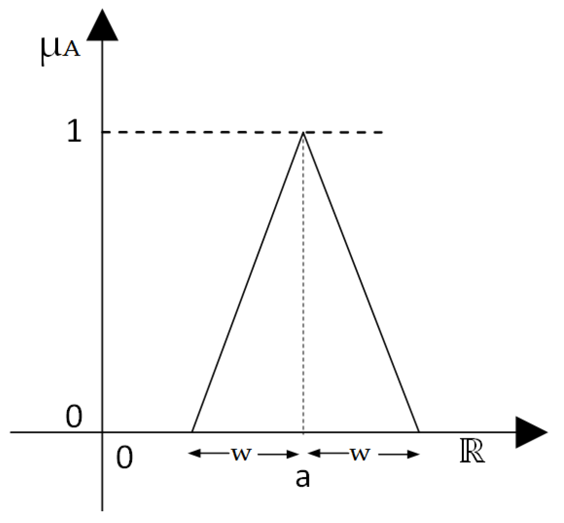
A special kind of fuzzy sets is the fuzzy numbers. In this work, fuzzy symmetrical triangular numbers are used which are special kinds of fuzzy numbers. The fuzzy symmetrical triangular numbers have the following membership function:

$${\mu }_A\left(x\right)=\{\begin{array}{l}1-\frac{\left|x-a\right|}{w},\hspace{0.17em}\hspace{0.17em}\hspace{0.17em}\begin{array}{cc}if& a-x\le x\le a+w\end{array}\\ 0,\begin{array}{cc}\begin{array}{cc}\begin{array}{cc}& \end{array}& \end{array}& \hspace{0.17em}\hspace{0.17em}\hspace{0.17em}\hspace{0.17em}\hspace{0.17em}\hspace{0.17em}\hspace{0.17em}\hspace{0.17em}\hspace{0.17em}otherwise\end{array}\end{array}$$

(3)

in which a is the centre and w the spreads of the fuzzy number (Figure 1).

2.2. Utilization of the Observed Probabilities by Using Fuzzy Regression in Case of Log Normal Distribution

Let an historical sample. The rank order method involves ordering the data from the largest hydrological value to the smallest hydrological value, assigning a rank of 1 to the largest value and a rank of N to the smallest value. Based on the Weibull 1939 empirical distribution to compute the plotting position probabilities, the cumulative exceedance probability can be assessed as follow:

$$P\left(Q\ge q\right)=\frac{m}{{\rm N}+1}$$

(4)

Therefore, the cumulative probability of non exceedance probability can be determined as follow [6]:

$$P\left(Q<q\right)=1-\frac{m}{{\rm N}+1}$$

(5)

Let now the log-normal theoretical probability distribution. To simplify the procedure, it is well-known that in case that the log-normal distribution is well-fitted to the observations, then the normal distribution with log-transformed data can be used instead of the lognormal distribution; which simply means that log-transformed data are implemented instead of the raw data and hence, the new auxiliary variable y, is normally distributed:

$$\ln q_{Tj}={\mathrm{y}}_{Tj}$$

(6)

Subsequently, based on the standardized normal variable Z of the normal distribution it holds:

$$\ln q_{Tj}=y_{Tj}=\overline{y}+s_y\cdot {{\rm Z}}_{{\rm T},j}=\lambda +\zeta \cdot {{\rm Z}}_{{\rm T},j}$$

(7)

In which as λ, ζ state the mean value and the standard deviation of the log transformed variable y correspondingly.

The critical points of the proposed methodology are the following next:

• Based on the observed probabilities, the standardized normal variable Z can be determined for each data.
• Based on Equation (7), a fuzzy linear regression model is implemented in order to determine a fuzzy relationship between the natural log of the cumulative discharge and the normalized variable Z (which corresponds to a probability). In addition, based on the fuzzy regression procedure, a fuzzy estimation regarding the mean value and the standard deviation of the log-transformed sample is achieved simultaneously [7]:

$${\tilde{y}}_{Tj}=\tilde{\overline{y}}+{\tilde{s}}_y\cdot {{\rm Z}}_{{\rm T},j}=\tilde{\lambda }+\tilde{\zeta }\cdot {{\rm Z}}_{{\rm T},j}$$

(8)

It should be clarified that since fuzzy symmetrical triangular numbers are selected as fuzzy coefficients hence, the mean value and the standard deviation are estimated as fuzzy symmetrical triangular numbers.

The uncertainty of the matching between the observed probabilities and the adopted theoretical probability distribution can be treated by using the fuzzy regression of Tanaka (1987) and hence, all the observed data will be included in the produced fuzzy band [8].

• The suitability of the proposed model can be estimated based on the magnitude of the fuzziness and furthermore by using mathematical distance norms to deal with the comparison between the unbiased estimators and the fuzzy estimation of the mean value and the standard deviation.

Considering the model of fuzzy regression itself let us provide some details. Although the standardized normal variable Z (independent variable) and the value of random variable (dependent variable) of the historical sample takes only crisp values, the fuzziness arises from the inclusion constraints that is, from the requirement that all the data must be included in the produced fuzzy band. In other words this means that the fuzziness is generated from the (expected) no identical matching between the theoretical probability distribution (in this article the log normal distribution) and the observed probabilities.

According to the extension principle, in case of fuzzy symmetrical triangular numbers as coefficients, the function ${\tilde{y}}_j$ will be also a fuzzy triangular number with the following centre (y_a,j) and width (w_yj) [5,9]:

$$\mathit{Centre}:y_{\mathrm{a}j}={\lambda }_{\mathrm{a}}+{\zeta }_{\mathrm{a}}\cdot {{\rm Z}}_{{\rm T},j}$$

(9a)

$$\mathit{Width}:w_{yj}=w_{\lambda }+w_{\zeta }\cdot \left|{{\rm Z}}_{{\rm T},j}\right|$$

(9b)

In which as $y_{\mathrm{a}j},{\lambda }_{\mathrm{a}},{\zeta }_{\mathrm{a}}$ state the central values of the corresponding variables and as $w_{yj},w_{\lambda },w_{\zeta }$ the corresponding spreads are meant.

The concept of inclusion is used to express the inclusion constraints. Thus, the inclusion of a fuzzy set A to the fuzzy set B with the associated degree $0\le h\le 1$ is defined as follow:

$$A\left[h\right]\subseteq B\left[h\right]$$

(10)

A physical interpretation of the level h is that an observation y_j is contained in the support interval of the corresponding fuzzy estimate, which has a degree of membership greater than h_j. The degree of fit of the estimated model to the entire data set is defined as the minimum of all these h_j, which is denoted as h [10].

The produced fuzzy band will contain all the observed data:

$$y_j\in \left[y_{\mathrm{h},\mathrm{j}}^{\mathrm{L}},\hspace{0.17em}{y}_{\mathrm{h},\mathrm{j}}^{\mathrm{R}}\right]$$

(11)

By taking into account the fuzzy arithmetic, for a selected level h, the inclusion constraints, in case that the decision variables (fuzzy coefficients) are selected to be fuzzy symmetrical triangular numbers, are equivalent to (e.g., [9,11,12]):

$$\{\begin{array}{l}\mathrm{{\rm I}}nclusion\hspace{0.17em}Constra\mathrm{int}s\\ \left({\lambda }_{\mathrm{a}}+{\zeta }_{\mathrm{a}}\cdot \hspace{0.17em}{\mathrm{{\rm Z}}}_{\mathrm{{\rm T}},j}\right)-\left(1-h\right)\left(w_{\lambda }+w_{\zeta }\left|{\mathrm{{\rm Z}}}_{\mathrm{{\rm T}},j}\right|\right)=y_{\mathrm{h},\mathrm{j}}^{\mathrm{L}}\le \ln {\mathrm{q}}_{\mathrm{j}}\\ \left(\hspace{0.17em}{\lambda }_{\mathrm{a}}+{\zeta }_{\mathrm{a}}\cdot \hspace{0.17em}{\mathrm{{\rm Z}}}_{\mathrm{{\rm T}},j}\right)+\left(1-h\right)\left(\hspace{0.17em}{w}_{\lambda }+w_{\zeta }\left|{\mathrm{{\rm Z}}}_{\mathrm{{\rm T}},j}\right|\right)={\mathrm{y}}_{\mathrm{h},\mathrm{j}}^{\mathrm{R}}\ge \ln {\mathrm{q}}_{\mathrm{j}}\\ w_{\lambda },\hspace{0.17em}{w}_{\zeta }\ge 0\end{array}$$

(12)

Since the fuzzy regression model of Tanaka (1987) is transformed to a constrained optimization problem, the assessment of the suitability of the model is based on the produced fuzzy band. Therefore, a significant small fuzzy band indicates a proper approach. Thus, Tanaka (1987) suggested the minimization of the sum of the produced fuzzy semi-spreads for all the data:

$$\min J\left(={\displaystyle \sum _{j=1}^M{w}_{yj}}=\left\{M\cdot w_{\lambda }+w_{\zeta }{\displaystyle \sum _{j=1}^M\left|{{\rm Z}}_{{\rm T},j}\right|}\right\}\right)\left(\mathrm{Objective}\mathrm{function}\right)$$

(13)

where M is the number of the observed data.

Based on the inclusion constraints, the produced fuzzy band must include all the observed data and this is one of the main advantages of the implementation of the fuzzy regression.

Two criteria are proposed in order to check the suitability of the achieved solution. The first one is sum of the produced fuzzy semi-spreads, J which indicates the fuzziness of the model. The second criterion of suitability, F, which examines how close is the central values of the mean value and the standard deviation to the unbiased (usual statistical) estimation of the same variables for the ln- transformed sample, $\widehat{\lambda },\hspace{0.17em}\widehat{\zeta }$:

$$F=\sqrt{\left({\lambda }_{\mathrm{a}}-\widehat{\lambda }\right){\hspace{0.17em}}^2+\left({\zeta }_{\mathrm{a}}-\widehat{\zeta }\right){\hspace{0.17em}}^2}$$

(14)

2.3. Categorization to Hydrogical Drough Based on the Return Period

As aforementioned, the thresholds of Z are used to define the thresholds of several drought categories (

Table 1. Classification of hydrological drought based on the random variable Z.

Category	Description	Criterion
0	Non-drought	Z ≥ 0.0
1	Mild drought	−1.0 ≤ Z<0.0
2	Moderate drought	−1.5 ≤ Z<−1.0
3	Severe drought	−2.0 ≤ Z<−1.5
4	Extreme drought	Z<−2.0

). In this article, based on the produced fuzzy curve (Equation (8)), the corresponding cumulative annual discharges, which can be seen as thresholds, are determined. It should be clarified that since the log–normal distribution is used (instead of the Gamma distribution), the normalized variable Z corresponds to a log-transformed cumulative discharge. The thresholds of Table 1 correspond to a fuzzy log-transformed cumulative discharge (based on Equation (8)) which can be compared with the current real log-transformed value of the cumulative discharge. Therefore, in this article the (fuzzy) thresholds of the annual cumulative discharge, $\ln {\tilde{V}}_k$ (considering the k threshold) are compared with the (crisp) observed annual cumulative discharge. Even if, there are many measures to compare fuzzy numbers, there are not all of them suitable to compare a fuzzy number with a crisp number. To address this problematic the reliability measure of Ganoulis, 2004 is adopted.

Let a system which has a resistance $\tilde{R}$ and a load $\tilde{L}$ as fuzzy numbers. A reliability measure or a safety margin of the system may be defined as being the difference between load and resistance. This is also a fuzzy number given by [13].

$$\tilde{M}=\tilde{R}-\tilde{L}$$

(15)

Hence, Ganoulis, 2004 has proposed a fuzzy measure of risk, $r$, which is defined as the region of the fuzzy safety margin, where values of $\tilde{M}$ are negative. Mathematically, this may be expressed as follows:

$$r=\frac{{\displaystyle \underset{m\le 0}{\int }{{\displaystyle \mu }}_{\tilde{M}}(m)dm}}{{\displaystyle \int {{\displaystyle \mu }}_{\widetilde{{\rm M}}}(m)dm}}$$

(16)

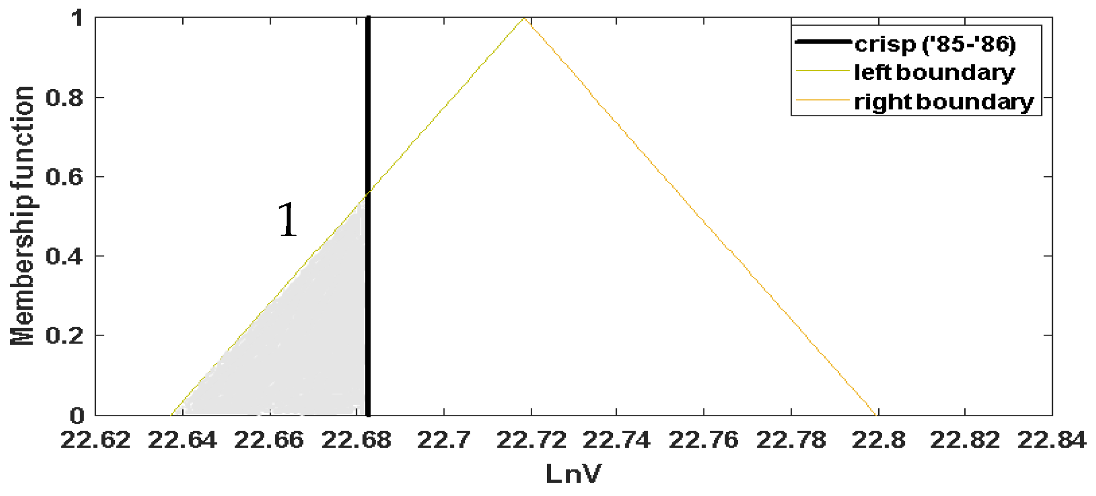
Let us return to the examined problem. Hence, the authors propose a measure $G_i{}_{,k}$, to indicate the degree according to which the examined hydrological year, i, has a cumulative annual discharge, $\ln V_i$ greater than the examined fuzzy threshold of drought k, $\ln {\tilde{V}}_k.$ It may be considered (Figure 2):

$$G_i{}_{,k}=\frac{{\displaystyle \underset{\ln V_k\le \ln V_i}{\int }{{\displaystyle \mu }}_{thresh,k}(\ln V)\hspace{0.17em}\hspace{0.17em}d\left(\ln V\right)}}{{\displaystyle \int {{\displaystyle \mu }}_{thresh,k}(\ln V)\hspace{0.17em}\hspace{0.17em}d\left(\ln V\right)}}=1-\frac{{\displaystyle \underset{\ln V_k\ge \ln V_i}{\int }{{\displaystyle \mu }}_{thresh,k}(\ln V)\hspace{0.17em}\hspace{0.17em}d\left(\ln V\right)}}{{\displaystyle \int {{\displaystyle \mu }}_{thresh,k}(\ln V)\hspace{0.17em}\hspace{0.17em}d\left(\ln V\right)}},\hspace{0.17em}\hspace{0.17em}{S}_i{}_{,k}=\frac{{\displaystyle \underset{\ln V_k\ge \ln V_i}{\int }{{\displaystyle \mu }}_{thresh,k}(\ln V)\hspace{0.17em}\hspace{0.17em}d\left(\ln V\right)}}{{\displaystyle \int {{\displaystyle \mu }}_{thresh,k}(\ln V)\hspace{0.17em}\hspace{0.17em}d\left(\ln V\right)}},\hspace{0.17em}$$

(17)

By the same way, a degree, $S_i{}_{,k}$, according to which the examined hydrological year, i, has a cumulative annual discharge smaller than the examined fuzzy threshold of drought k can be considered. In Figure 2 the grey hatched area (which is marked with (1)) denotes the numerator whilst the dominator is equal to the total area. For instance, regarding the hydrological year 1985–1986, G_{85–86,Z =−1} =1 and S_{85–86,Z = 0} = 0.8487>0.5.

3. Implementation of the Proposed Methodology: Annual Cumulative Streamflow Time Sequence

The case under investigationis the northern region of Prefecture Evros (Figure 3). The annual cumulative streamflow, which is derived from the monthly discharges of Evros River at Pythio’sbridge, is studied. Evros River (Maritsa or Meric) is one of the largest river of Balcan Peninsula in terms of length, since it crosses the Bulgarian, Greek and Turkish borders. It rises in the Rila Mountains in Western Bulgaria and has its outlet in the Aegean Sea. It serves as a natural borderline between Greece and Turkey [14]. Its total watershed area is equal to 53,000 Km², while the 6% of this is in Greek territory.

Methodology Steps

The proposed methodology is implemented using the following steps:

• Based on the monthly discharges, the annual cumulative volumes of streamflow are calculated and then they are transformed to logarithmic values.
• Based on the cumulative empirical (observed) distribution, the standardized normal variable Z is calculated for each examined hydrological year.
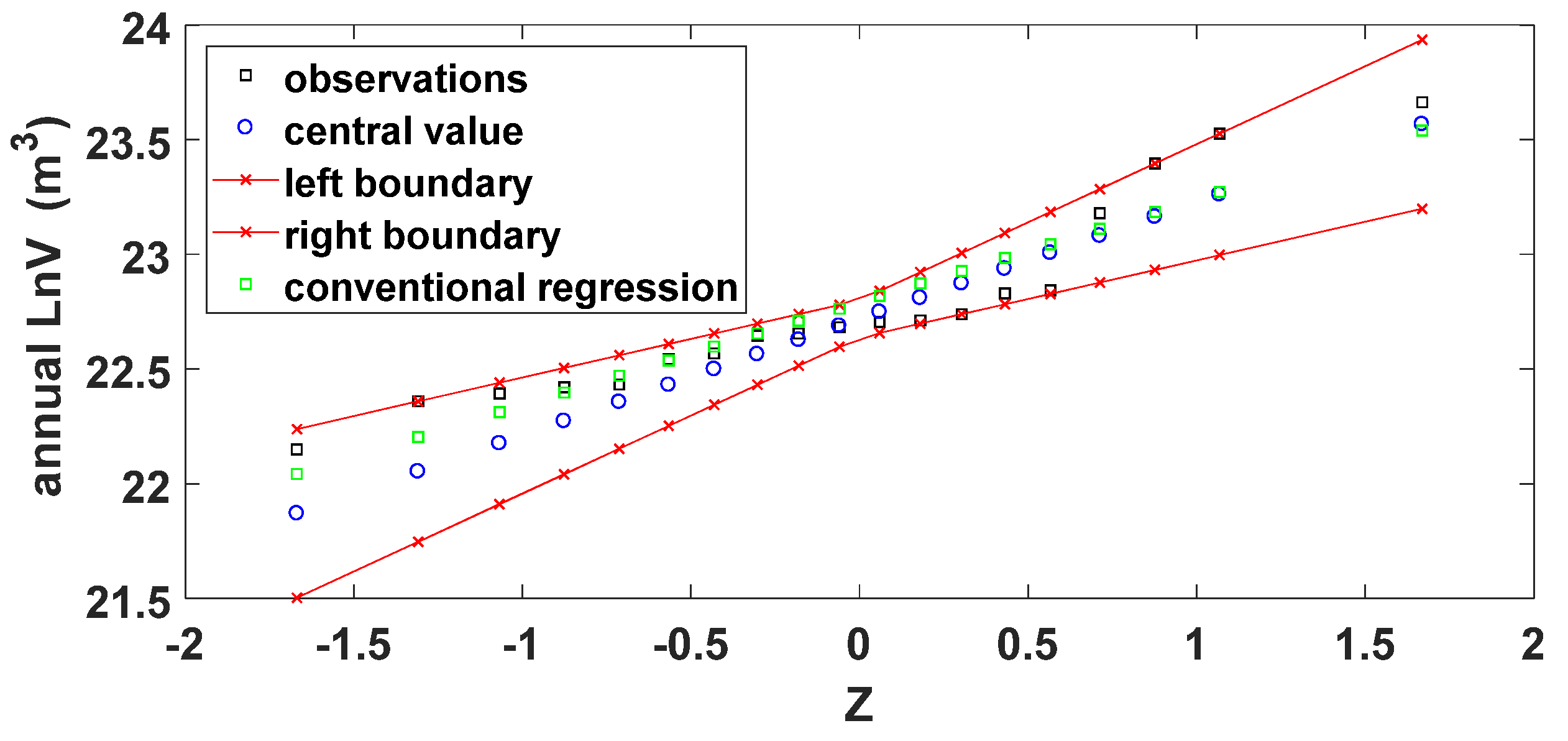
• The fuzzy linear regression model of Tanaka (1987) [9] is applied (Figure 4) between the standardized normal random variable Z and the log-transformed annual cumulative discharge. The produced fuzzy coefficients constitute fuzzy symmetrical triangular numbers. Its values can be seen as a fuzzy assessment of the mean value and the standard deviation. The fuzzy relation that was determined is (Figure 4):

  $$y_{Tj}={\left(22.72,0.081\right)}_L+{\left(0.51,0.172\right)}_L{Z}_{Tj}$$

  (18)

  in which the brackets state the fuzzy symmetrical triangular numbers (which are a special case of the L-fuzzy numbers) and within the bracket the first term symbolizes the central value and the second term the spreads of the aforementioned fuzzy numbers.

4.

The suitability is checked according to the value of the objective function, J and the measure according to Equation (14). The objective function equal to J =4.08 and as it can be seen from Figure 4 the uncertainty is not no functional. The unbiased estimation of the mean value and the standard deviation for the logs transformed sample are $\widehat{\lambda }\hspace{0.17em}=22.80,\hspace{0.17em}\widehat{\zeta }=0.44$ and therefore, the centers of the fuzzy coefficients are close to the unbiased estimations.

$$F=\sqrt{{\left({\lambda }_a-\widehat{\lambda }\right)}^2+{\left({\zeta }_a-\widehat{\zeta }\right)}^2}=\sqrt{{\left(22.72-22.80\right)}^2+{\left(0.51-0.44\right)}^2}=0.106$$

(19)

5.

Based on drought classification (Table 1) the ln of the annual cumulative discharge which correspond to the normalised variable Z equal to −2, −1.5, −1 and 0 (Table 1) are calculated based on Equation (18). Therefore, according to the corresponding values of Z, the fuzzy thresholds of drought are determined based on the produced fuzzy curve.

6.

The observed cumulative annual discharge is compared with the aforementioned thresholds to drought. From a mathematical point of view the observed cumulative annual discharges are crisp numbers whilst the thresholds are fuzzy numbers. The comparison is started from the lowest to the upper values, that is, by following an ascending procedure.

There also some cases where the comparison between the fuzzy threshold and the crisp annual cumulative discharge is not precise. Hence the following criterion is adopted in this analysis:

$$\ln V_i\mathrm{overcomes}\ln {\tilde{V}}_k\mathrm{if}\mathrm{it}\mathrm{holds}:G_i{}_{,k}=\frac{{\displaystyle \underset{\ln V_i\ge ln{V}_k}{\int }{{\displaystyle \mu }}_{thresh,k}(\ln V)\hspace{0.17em}\hspace{0.17em}d\left(\ln V\right)}}{{\displaystyle \int {{\displaystyle \mu }}_{thresh,k}(\ln V)\hspace{0.17em}\hspace{0.17em}d\left(\ln V\right)}}>0.5$$

(20)

In

Table 2. Drought classification based on the fuzzy measure G_i,k and S_i,k.

Comparison of Crisp and Fuzzy Streamflow Values
Hydrological Year	LnVi(m3)	Greater than the Lower Thresh. of the Category	Smaller than the Upper Thresh. of the Category	Drought Categories
1985–1986	22.6826542	1	0.8787	mild drought
1986–1987	22.7118034	1	0.5860	mild drought
1987–1988	22.7391331	0.7188	1	mildly wet
1988–1989	22.5682508	1	1	mild drought
1989–1990	22.3941092	0.9608	1	mild drought
1990–1991	22.7059660	1	0.6472	mild drought
1991–1992	22.5434611	1	1	mild drought
1992–1993	22.4211663	0.9855	1	mild drought
1993–1994	22.1499070	0.9075	0.7112	moderate drought
1994–1995	22.8424773	1	1	mildly wet
1995–1996	23.1777925	1	0.6780	mildly wet
1997–1998	23.5255678	0.6216	0.8750	severely wet
1998–1999	23.3953991	0.9422	0.7262	moderately wet
1999–2000	22.6456004	1	0.9950	mild drought
2000–2001	22.3591526	0.9118	1	mild drought
2001–2002	22.4334485	0.9928	1	mild drought
2003–2004	22.8287708	1	1	mildly wet
2004–2005	23.6016702	0.7887	0.7688	severely wet
2005–2006	23.6618808	0.8896	0.6638	severely wet
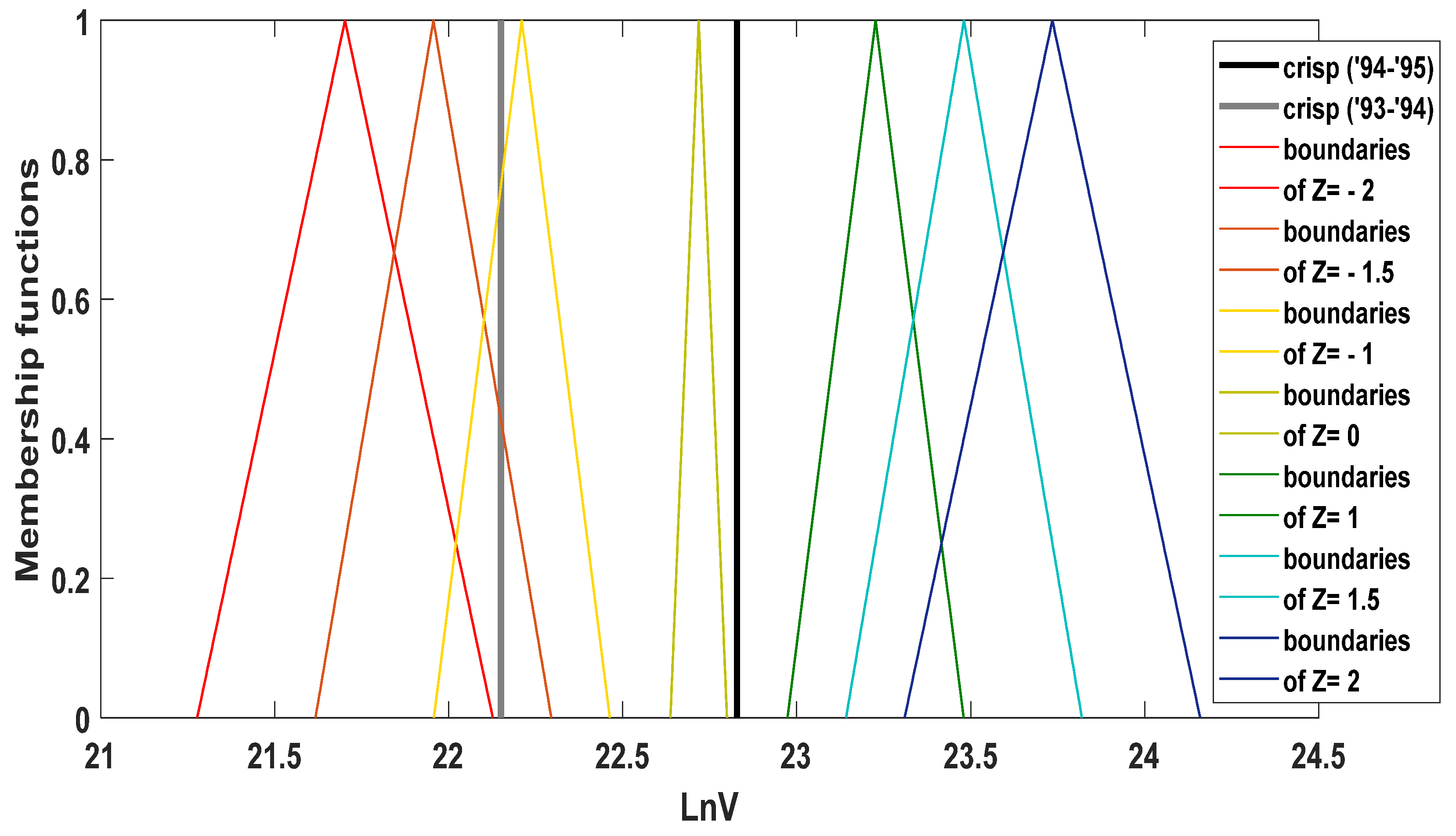
2006–2007	22.6549724	1	0.9780	mild drought

, the results of the above implementation steps are presented. It is observable that that because of the overlapping of the fuzzy lnV_k values (Figure 5), the frontiers between the categories are overlapped to some degree. In any case it seems more reasonable to adopt fuzzy thresholds between the categories to drought, compare with crisp, as the conventional methodology do. It is worth noting that although there are some cases where the comparison between the fuzzy threshold and the crisp annual cumulative discharge is not precise, in most of them, the G_i,k index has values which are discernible different from 0.5.

4. Concluding Remarks

The uncertainty of the coupling between the observed probabilities and the adopted theoretical probability distribution can be treated by using the fuzzy regression model of Tanaka (1987), where all the observed data are included in the produced fuzzy band. By using the log-normal probability distribution together with the fuzzy regression, an estimation of the mean value and the standard deviation can be achieved simultaneously. As it is seen from the case study, two criterion of suitability are established in order to check the suitability of the adopted theoretical probability density with fuzzy numbers as parameters. The first criterion of suitability is based on the width of the produced fuzzy band and the second is based on the distance between the unbiased estimation of the mean value and the standard deviation with the central values of the estimated fuzzy quantities.

Hence, by using the standardized indices, Z, to categorize the drought, the corresponding thresholds to drought can be determined as fuzzy numbers. The proposed methodology is successfully applied in case of the Evros river regarding the cumulative annual discharge. The observed cumulative annual discharge is compared with the aforementioned thresholds to drought. This comparison is taken place by using the proposed measure of comparison between fuzzy number and crisp number, which exploits all the information of the membership function. Finally, an efficient classification to drought is achieved following the proposed methodology although the fuzziness is taken into account.

References

- Wilhite, D.; Sivakumar, M.; Pulwarty, R. Managing drought risk in a changing climate: The role of national drought policy. Weather Clim. Extrem. 2014, 3, 4–13. [Google Scholar] [CrossRef]
- Angelidis, P.; Maris, F.; Kotsovinos, N.; Hrissanthou, V. Computation of Drought Index SPI with Alternative Distribution Functions. Water Resour. Manag. 2012, 26, 2453–2473. [Google Scholar] [CrossRef]
- Tsakiris, G.; Pangalou, D.; Vangelis, H. Regional drought assessment based on the Reconnaissance Drought Index (RDI). Water Resour. Manag. 2007, 21, 821–833. [Google Scholar] [CrossRef]
- Nalbantis, I.; Tsakiris, G. Assessment of Hydrological Drought Revisited. Water Resour. Manag. 2009, 23, 881–897. [Google Scholar] [CrossRef]
- Spiliotis, M.; Hrissanthou, V. Fuzzy and crisp regression analysis between sediment transport rates and stream discharge in the case of two basins in northeastern Greece. In Regression Analysis: Introduction, Applications and Theory; Nova Science Publishers: New York, NY, USA, 2018; in press. [Google Scholar]
- Chow, V.; Maidment, D.; Mays, L. Applied Hydrology, Hill International ed.; McGraw: Singapore; New York, NY, USA, 1988; pp. 394–398. [Google Scholar]
- Spiliotis, M.; Papadopoulos, B. A hybrid fuzzy probabilistic assessment of the extreme hydrological events. In Proceedings of the 15th International Conference of Numerical Analysis and Applied Mathematics (ICNAAM 2017, Thessaloniki, Greece, 25–30 September 2017. [Google Scholar]
- Spiliotis, M.; Angelidis, P.; Papadopoulos, B. A Hybrid Fuzzy Regression-Based Methodology for Normal Distribution (Case Study: Cumulative Annual Precipitation). In Proceedings of the 14th IFIP International Conference on Artificial Intelligence Applications and Innovations (AIAI), Rhodes, Greece, May 2018; Iliadis, L., Maglogiannis, I., Plagianakos, V., Eds.; Springer International Publishing: Berlin, Germany, 2018; pp. 568–579. [Google Scholar]
- Tanaka, H. Fuzzy data analysis by possibilistic linear models. Fuzzy Sets Syst. 1987, 24, 363–375. [Google Scholar] [CrossRef]
- Moskowitz, H.; Kim, K. On assessing the h value in fuzzy linear Regression. Fuzzy Sets Syst. 1993, 58, 303–327. [Google Scholar] [CrossRef]
- Tsakiris, G.; Tigkas, D.; Spiliotis, M. Assessment of interconnection between two adjacent watersheds using deterministic and fuzzy approaches. Eur. Water 2006, 15, 15–22. [Google Scholar]
- Tzimopoulos, C.; Papadopoulos, K.; Papadopoulos, B. Fuzzy Regression with Applications in Hydrology. Int. J. Eng. Innov. Technol. (IJEIT) 2016, 5, 69–75. [Google Scholar]
- Ganoulis, J. Integrated Risk Analysis for Sustainable Water Resources Management. In Comparative Risk Assessment and Environmental Decision Making; Linkov, I., Ramadan, A.B., Eds.; Kluwer Academic: Norwell, MA, USA, 2004; Volume 38, pp. 275–286. [Google Scholar]
- Angelidis, P.; Kotsikas, M.; Kotsovinos, N. Management of Upstream Dams and Flood Protection of the Transboundary River Evros/Maritza. Water Resour. Manag. 2010, 24, 2467–2484. [Google Scholar] [CrossRef]
Figure 1.
Fuzzy triangular symmetrical number.
Figure 2.
Measure value resulting from the ratio of the hatched area to the total area is less than 0.50 for the year 1985–1986.
Figure 3.
Transboundary Evros river and its tributaries. The examined data are derived from Pythio’s bridge (41°21′43.51″ N 26°37′51.67″ E) (from Angelidis et al., 2010).
Figure 4.
Observed data, fuzzy and conventional (crisp) regression between the annual cumulative logarithmic streamflow values and the standardised random variable Z.
Figure 5.
Fuzzy thresholds of drought regarding the values of Z (presented in Table 1) and the (crisp) annual cumulative discharge for the hydrological year, 94–95 and 93–94.