Impact of Climate Change on Groundwater Management in the Northwestern Part of Uzbekistan


1
Leibniz Centre for Agricultural Landscape Research (ZALF), Eberswalder Straße 84, 15374 Müncheberg, Germany
2
Tashkent Institute of Irrigation and Agricultural Mechanization Engineers (TIIAME), Kary-Niyaziy 39, Tashkent 100000, Uzbekistan
*
Author to whom correspondence should be addressed.
Agronomy 2020, 10(8), 1173; https://doi.org/10.3390/agronomy10081173
Submission received: 8 July 2020
/
Revised: 29 July 2020
/
Accepted: 7 August 2020
/
Published: 10 August 2020
(This article belongs to the Special Issue The Adaptation of Agriculture to Climatic Change)
Abstract
:Global climate change can have a significant impact on the development and sustainability of agricultural production. Climate scenarios indicate that an expected increase in air temperature in semiarid Uzbekistan can lead to an increase in evapotranspiration from agricultural fields, an increase in irrigation water requirements, and a deterioration in the ameliorative status of irrigated lands. The long-term mismanagement of irrigation practices and poor conditions of drainage infrastructure have led to an increase in the water table and its salinization level in the northwestern part of Uzbekistan. This article presents the results of an analysis of the amelioration of irrigated lands in the Khorezm region of Uzbekistan as well as the modeling of the dynamics of water table depths and salinity levels using the Mann–Kendall trend test and linear regression model. The study estimated the water table depths and salinity dynamics under the impact of climate change during 2020–2050 and 2050–2100. The results show that the water table depths in the region would generally decrease (from 1.72 m in 2050 to 1.77 m by 2100 based on the Mann–Kendall trend test; from 1.75 m in 2050 to 1.79 m by 2100 according to the linear regression model), but its salinity level would increase (from 1.72 g·L−1 in 2050 to 1.85 g·L−1 by 2100 based on the Mann–Kendall trend test; from 1.97 g·L−1 in 2050 to 2.1 g·L−1 by 2100 according to the linear regression model). The results of the study provide insights into the groundwater response to climate change and assist authorities in better planning management strategies for the region.
1. Introduction
Central Asian countries are among the states that are vulnerable to climate change. Mean annual air temperature increases have already been observed across Central Asia due mainly to natural causes [1]. Warming trends are more pronounced in the lower elevation plains and intermountain valleys than at higher elevations [2]. The warming across Central Asia is expected to exceed the global average, with the southernmost areas experiencing a greater shift in temperatures and the northernmost parts showing a less pronounced shift. According to some climate scenarios, a 2.5 °C increase is expected in the summer temperature in Central Asia towards the end of this century [3]. Moreover, the annual mean precipitation in Central Asia is projected to continuously increase by 14.51% (8.11 to 16.9%) by the end of the 21st century, and this precipitation would mainly fall outside the regular crop growing period (November–March) [4]. In Uzbekistan, the rate of increase in air temperature has been of 0.27 °C over 10 years [5].
Climate change and its impact on agricultural production have been widely researched by domestic and foreign scientists [6,7]. For instance, a number of renowned scientists have placed major emphasis on the study of global warming [8,9,10]. Much attention is paid to problems related to the adaptation of agriculture to climate change, such as the introduction of new crops, crop rotation changes, alterations in the intensity of tillage practices, optimization of fertilization, and changes from grassland to arable land [11,12,13], which are also in line with the findings in Europe [14].
Academics and governments generally agree that climate change also impacts the dynamic changes in water table depths [15,16,17,18,19]. Prolonged droughts and low levels of rainfall may cause a significant decline in water table depth [20]. In fact, the water table is a useful water resource during drought periods and for upland crop cultivation [21,22,23]. Climate change and variability may threaten environmental sustainability and the livelihoods of billions of people around the world [24]. Along with climate change, population increases have imposed pressure on irrigated agriculture, which in turn has resulted in excessive groundwater extraction for irrigation purposes [25,26].
Irrigated agriculture plays an important role in the economy of the Khorezm region of Uzbekistan. Due to the continuous population growth in the region, the role of irrigated agriculture as the main source of food security is noticeably increasing; however, at the same time, pressure on the available water and land resources is also increasing. The high degree of salinization and waterlogging of the land, as well as the increasingly acute shortage of water resources, jeopardize the sustainability of agriculture in this region [27]. According to the Food and Agriculture Organization (FAO) of the United Nations, almost all irrigated lands in Khorezm are saline or subject to secondary salinization processes as a result of the level of the salinized water table quickly rising to the surface of the earth [28]. A high water table level occurs when there are small surface slopes and as a result of the high water conductivity of sandy soils, although the main reason is ineffective water management. For example, scarce water resources during 1995, 2000–2001, and 2008 clearly demonstrated that there was an urgent need for a transition from old, ineffective methods of managing irrigated agriculture to new, advanced technologies suitable for the conditions of Khorezm [29].
The rising levels of the salinized water table significantly affect soil fertility. In Uzbekistan, the total area of irrigated land in the groundwater zone with a salinity up to 3.0 g·L−1 is 3.35 million ha or 77.98%. In the Khorezm region, there are approximately 0.26 million ha of irrigated lands, of which the groundwater is covered in approximately 0.22 million ha, which have a salinity level of between 1.0–3.0 g·L−1 [30]. Shallow water table depth with high salinity level causes disruption to the development of crop productivity in the region [31]. In order to combat salinity issues, salt-tolerant crops are widely studied in the region [32,33]. Moreover, reducing the level of highly salinized water table through different irrigation methods are also studied by some scholars [34,35]. In this research, however, our main focus lies on the analysis of climate change and its impact on the dynamics of the water table depths and salinity (mineralization) levels.
Because the irrigated lands of the Khorezm region are 100% saline, the region was taken as the focus of this research. In this study, we primarily focused on irrigated lands; therefore, other land categories, including forest and pasture lands, were not considered. The total land area in Uzbekistan is approximately 44.7 million ha, of which 62.6% is agricultural land, 7.7% is forestland, and 29.7% belongs to other categories (e.g., industrial, historical, and water resources) [36]. In comparison to other studies in the region [37,38,39,40,41], this research aims to analyze meteorological data for the period of 1928–2017, including air temperature (°C), precipitation (mm), absolute humidity (g·m−3), relative humidity (%), wind speed (m·s−1), and land surface temperature (°C), using a linear regression model as well as a Mann–Kendall trend test over a 10-year average. We also analyzed the impacts of climate change, not only on the dynamics of the water table depths, but also on the salinity. As a result, water table depths and salinity will serve as additional tools for developing management strategies and assessing the ameliorative status of irrigated lands in the region. In this research work, the assumption included that the warming of the climate may lead to the decline in water table depth and increase in the level of salinity.
2. Materials and Methods
2.1. Case Study Area
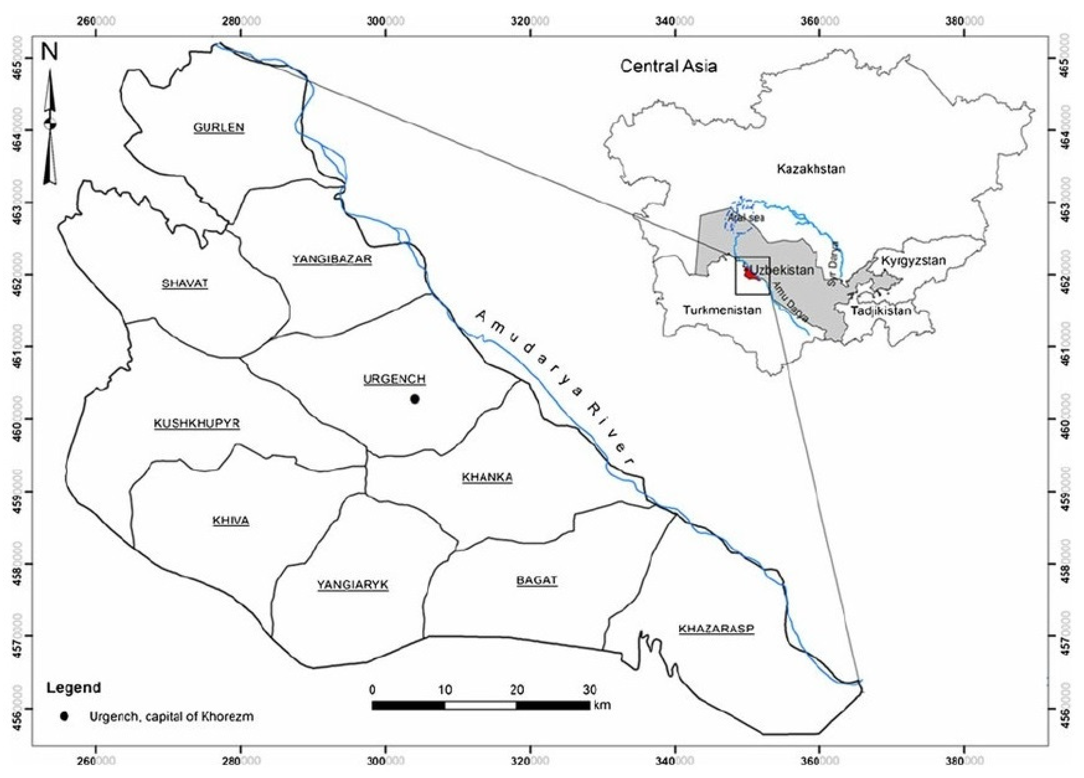
The Khorezm region is situated in the northern part of Uzbekistan, close to the Aral Sea, and in the downstream of the Amu Darya River. The region is divided into 10 administrative districts, with the capital Urgench serving as an administrative center. The remaining districts include the Bagat, Gurlen, Kushkupyr, Urgench, Khazarasp, Khanka, Khiva, Shavat, Yangiaryk, and Yangibazar districts (Figure 1). All districts in the region are part of the study area. We took the average data for all 10 districts and generalized the data for the entire region. Geographically, the region is located in a semi-desert zone in Central Asia, characterized by an extreme continental climate, spreading between latitudes 41°00′ to 42°10′ N and longitudes 60°02′ to 61°44′ E.
The climatic information for the study area was collected from the Khiva meteorological station. According to the data, the average air temperature in the crop growing period (April–October) during 1928–2017 was 21.3 °C. Moreover, the lowest average monthly air temperature was observed in the winter, while the highest average monthly air temperature was observed in July, i.e., −2.8 °C and 27.8 °C, respectively. Finally, the maximum average precipitation was 18.2 mm in March, and the minimum was 1.2 mm in July.
The average annual rainfall during the study period (1928–2017) was observed as 100 mm, which fell mainly during the non-crop growing period. Furthermore, the average annual evaporation was approximately 1500 mm [42]. Therefore, irrigated agriculture plays a key role in the region. Water flows from the Amu Darya River through a dense network of irrigation canals. The study area is one of the final recipients of irrigated water because of its location in the lower reaches of the river basin. The water supply for irrigation from the Amu Darya River in the region has recently been unstable [38]. This instability is because the river flow has significantly decreased, which is associated with increased upstream water consumption, an unpredictable climate, and frequent droughts [43].
These events have already caused serious setbacks in 2000, 2001, and 2008 [44]. A total of 1.8 million people live in the region, of which 70% are engaged in crop production, animal husbandry, and horticulture [45]. Cotton and winter wheat are the two main crops grown in this area. Cotton is one of the main cash crops in Uzbekistan, while wheat is the country’s main grain crop [46]. Other cultivated crops are rice, watermelon, alfalfa, corn, sorghum, and grapes. Orchards are scattered throughout the region. The growing season for most crops in the region is during April–September, while winter wheat is grown during October–July. The harvest schedule was obtained from the regional land administration authority in the Khorezm region of the Republic of Uzbekistan.
The data on water table depths were generated based on 1200 monitoring wells, which are under the jurisdiction of the Khorezm Ameliorative Expedition.
2.2. Linear Regression Model
Observations carried out on a biological object using correlation-related signs x and y can be represented by points on the plain, by constructing a system of rectangular coordinates. As a result, a type of scatter diagram is prepared, which makes it possible to judge the form and tightness of the connection between the varying attributes [47].
In many instances, this relationship seems to be a straight line or can be approximated by a straight line. The linear relationship between variables x and y is described by an equation of the general form y = a + bx1 + cx2 + dx3 +…, where a, b, c, d… are the parameters of the equation that determine the relations between the arguments x1, x2, x3…, xn, and function y. [48].
We described the relationship between temperature (y) and year number (x) with a simple linear regression model:
In the linear regression Equation (1), a is a free term, and parameter b determines the slope of the regression line with respect to the axes of rectangular coordinates. In analytical geometry, this parameter is called the angular coefficient, and in biometrics, it is called the regression coefficient.
The formula for calculating the correlation coefficient is constructed in such a way that if the relationship between the features is linear, the Pearson coefficient accurately establishes the tightness of this relationship. Therefore, it is also called the Pearson linear correlation coefficient [49].
The strength of the linear relationship between temperature and time was described with Pearson’s correlation coefficient [50]:
where xi is the value taken by the variable X, yi is the value taken by the variable Y, is the mean of X, and is the mean of Y.
Prognostic extrapolation was performed after the results were regionalized and averaged. It was based on the principles of simple linear modeling:
where —predicted water table depth or salinity, —observed data, and —prediction coefficient.
From the above equation, we derive the function of data extrapolation between two points. As a result of this function, we obtain future increasing or decreasing quantity values:
The prognostic extrapolation was based on the approach of average forecasting. With this approach, all future values of the time series studied are equal to the mean:
where are regional values for observed water table depth and salinity, and T is prospective years (five-year interval).
2.3. Mann–Kendall Trend Test
The Mann–Kendall test and Sen’s slope were used to identify water table trends and to model their depths in a timely manner to predict subsequent water levels [51,52]. It is a widely accepted statistical tool to predict and analyze different pollutants statistics, retrieved over time for steadily decreasing or increasing trends [53,54,55,56]. Originally developed by Mann [57] and later, reworked by Kendall [58], the test is defined as “the null hypothesis of this non-parametric test defines no monotonic trend in data, and alternate hypothesis states an existence of a positive, negative or non-null trend” [59].
Most statistical tests of the monotonic trend in hydrological time series are affected by some of the following problems: abnormal data, missing values, seasonality, censoring and serial dependence, and sequential correlation [60]. Rising water tables are likely to be associated with recurrent droughts and rising temperatures [61]. Two possibilities were used to compare and evaluate the impact of climate change: (i) analysis of trends in the historical climate and the hydrological data obtained from regular monitoring systems using the Mann–Kendall test; and (ii) the linear regression model [62]. We used temperature as a main explanatory variable and made some scenario of how future temperatures would impact on water table depths and salinity changes.
The Mann–Kendall trend test is a ranking-based nonparametric test used to assess the significance of a trend. The null hypothesis H0 is that the sample is chronologically ordered, independent, and normally distributed. The statistics S has the following form [63]:
where:
If n ≥ 40, this indicates that S is asymptotically normally distributed with a mean of 0 and a variance described by the following equation:
where t is the size of this related group, and the sum of all related groups in the data sample. The standardized verification statistic K can be calculated using the equation:
The standardized statistic K obeys the standard normal distribution law with a mean zero value and unit variance. The probability value P of the statistic K of the sample can be estimated using the normal integral distribution function:
For independent data sampling without a trend, the value of P should be equal to 0.5. A sample with a large positive trend will have a P close to 1.0; a sample with a large negative trend will have a P close to 0.0. If the data samples have an in-line correlation, then the data must first be “cleared”, and the correction obtained is applied to calculate the variance [63].
In this study, a future prediction was made by calculating the percentage change in the linear Sen’s slope based on the median of the data:
where β is Sen’s slope estimate, and xj is j-th observation. With an uptrend, the value of β is positive, and with a downtrend, β is negative.
To do this, a linear relationship of changes in water table depth under the condition of air temperature changes over 5-year and 10-year period intervals was identified.
The determined slope between the two variables was determined as a percentage correlation, and extrapolative changes were determined by adding the arithmetic to the available averages.
To do so, each time series is a variable in , based on the solution of the following equation:
where a, b are the averages of the quantities in the time interval (b > a), m is the number of pairs of data, and is the slope for each pair of data and the median value of all calculated slopes is Sen’s slope estimator.
Based on the above, the average change in the general trend was determined with the following equation [59]:
Based on this equation, the Mann–Kendall test can be used to predict changes in water table depth and salinity that depend on the temperature on slopes. This prediction methodology was developed in order to compare the accuracy of the linear extrapolation method analyzed unilaterally. This analysis was performed using XLSTAT software.
3. Results and Discussion
Statistical analysis of the average annual air temperature in the Khorezm region was conducted from 1928 to 2017. As a result, the 90-year average was 12.961 °C, the maximum was 14.983 °C, and the minimum was 10.558 °C. The standard deviation was 1.020 (Table 1). There are two meteorological stations in the Khorezm region: Urgench and Khiva. We used only one station, located in Khiva district, to assess the climate situation. The main rationale behind using the Khiva meteorological station is: (a) data accessibility and accuracy, and (b) availability of long-term data.
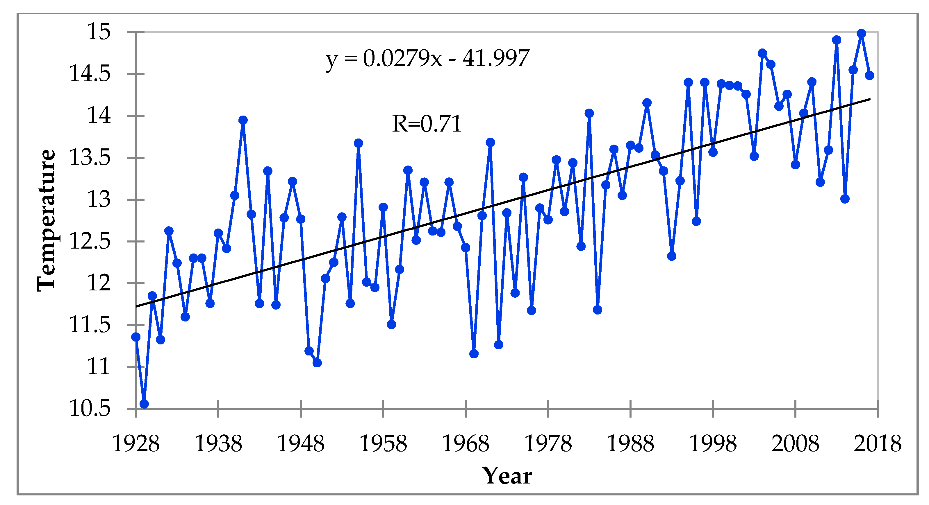
Based on the trends in the linear analysis of air temperature changes in 1960–2017, the correlation coefficient was found to be 0.56 [64]. In Kashmir, the correlation coefficient was 0.68, as determined by the air temperature analysis from 1980 to 2016 [65]. In 1949–2010, California’s Central Valley had a correlation coefficient of 0.57 [66]. In our research, the correlation coefficient calculated from the dynamics of the average air temperature change between 1928 and 2017 was equal to R = 0.71. This result shows that the average air temperature is directly proportional to the year. Figure 2 shows that the degree of linear dependence is positively related to the length of the observation period.
As a result of the literature analysis, we presented the average values of the climate indicators in Uzbekistan. In addition, the study analyzed the average, maximum, and minimum values of each climate indicator, and the results are presented in Table 2.
When comparing our results with the values in some other countries, for instance, in India, the maximum temperature for the observed period from 1980 to 2017 showed a slight warming or increasing trend (Sen’s slope = 0.29), while the minimum temperature showed a cooling trend (Sen’s slope = −0.006) [37]. In this study, a detailed analysis of the per ten-year average data for 1928–2017 showed that the average air temperature, maximum temperature, and minimum temperature of the Sen’s slope were 0.284 °C, 0.246 °C, and 0.423 °C, respectively. The land surface average and minimum temperatures show that Sen’s slopes are 0.506 °C and 0.17 °C, respectively, while the absolute maximum trend shows a cooling trend (Sen’s slope = −0.708 °C). The average precipitation during the 10-year period showed a decreasing trend (Sen’s slope = −0.617). Humidity also showed an increasing trend (Table 2).
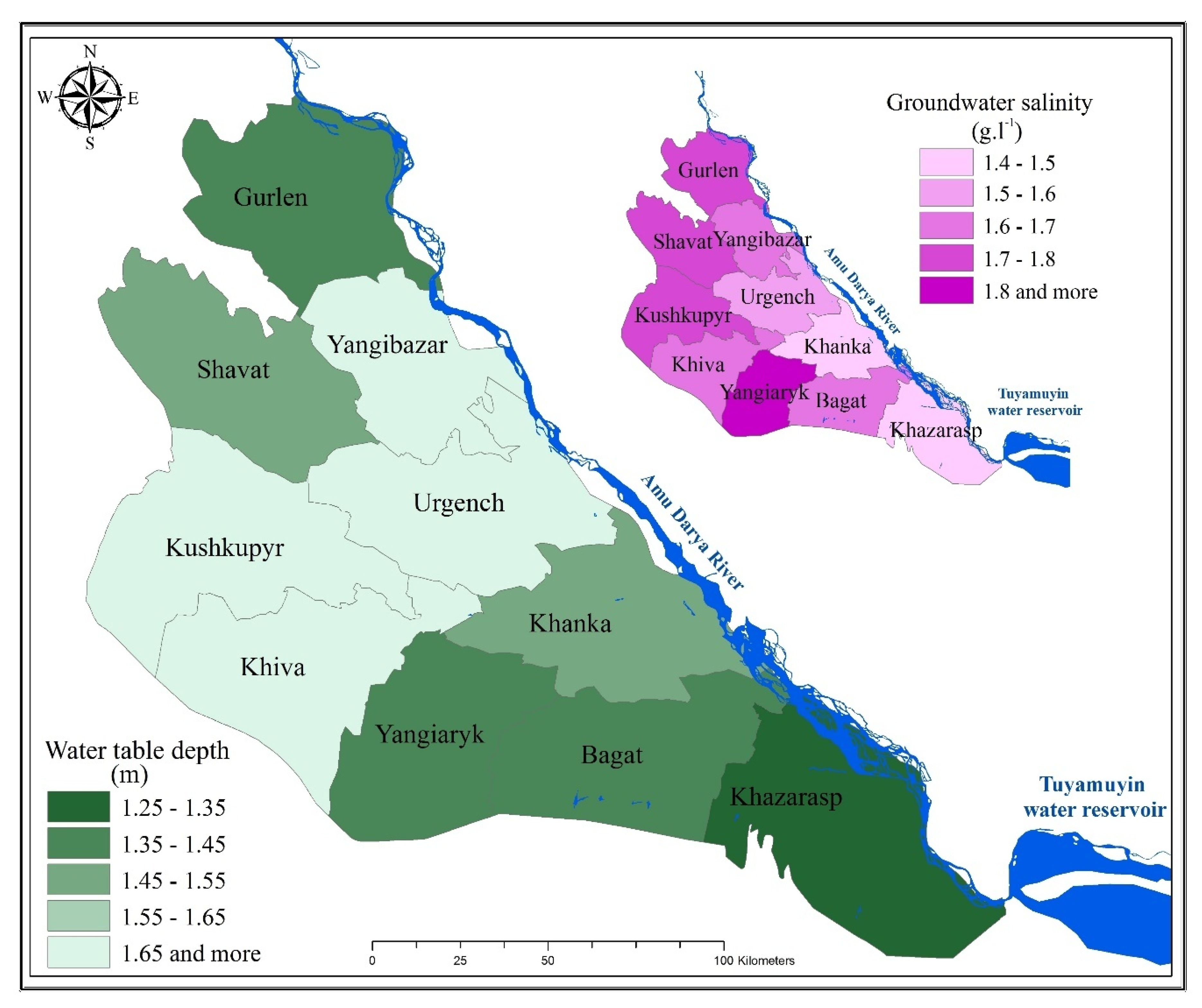
The analysis of the average water table depth and salinity in the districts of the Khorezm region showed variations during the study period. For instance, in the areas close to the Tuyamuyin Reservoir and the Amu Darya River, the water table depths were relatively close to the surface, i.e., 1.25–1.35 m in the Khazarasp district and 1.35–1.45 m in the Gurlen district. In the Bagat and Yangiaryk districts, the depths were 1.35–1.45 m due to the use of furrow irrigation technology. The average water table depth in the Shavat district was approximately 1.45–1.55 m, while that in the Khanka district was 1.55–1.65 m. In the Khiva, Kushkupyr, Yangibazar, and Urgench districts, the average depth was found to be 1.65 m and below. Additionally, the analysis of groundwater salinity indicated salinities of 1.4–1.5 g·L−1 in the Khazarasp and Khanka districts, which can be explained by their position near the Tuyamuyin Reservoir. In the Urgench district, the salinity was 1.5–1.6 g·L−1; in the Yangibazar district, the salinity was 1.6–1.7 g·L−1; and in the Khiva and Bagat districts, the salinity was approximately 1.7–1.8 g·L−1. The groundwater salinity in the Kushkupyr, Shavat, and Yangiaryk districts was found to be 1.8 g·L−1 or higher due to the poor drainage and high salinity (Figure 3).
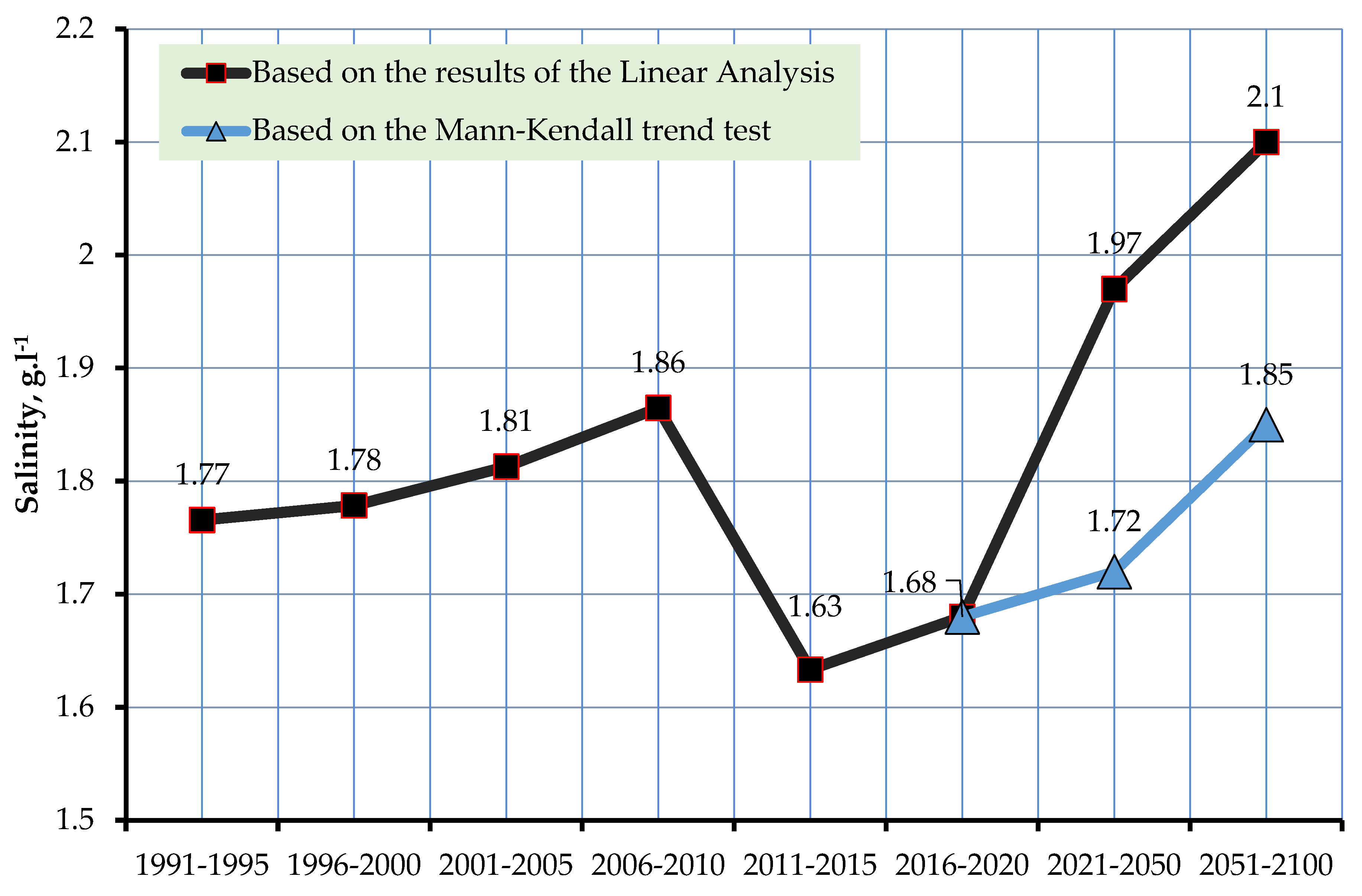
The ameliorative status of land and, in particular, the assessment of the impact of climate on the level and salinity of the groundwater in irrigated lands, requires complex decisions (of which salinity and waterlogging are part). Therefore, predictions of groundwater salinity and its depth level are important source of data for policy-makers in better planning management strategies for the region (Figure 4 and Figure 5).
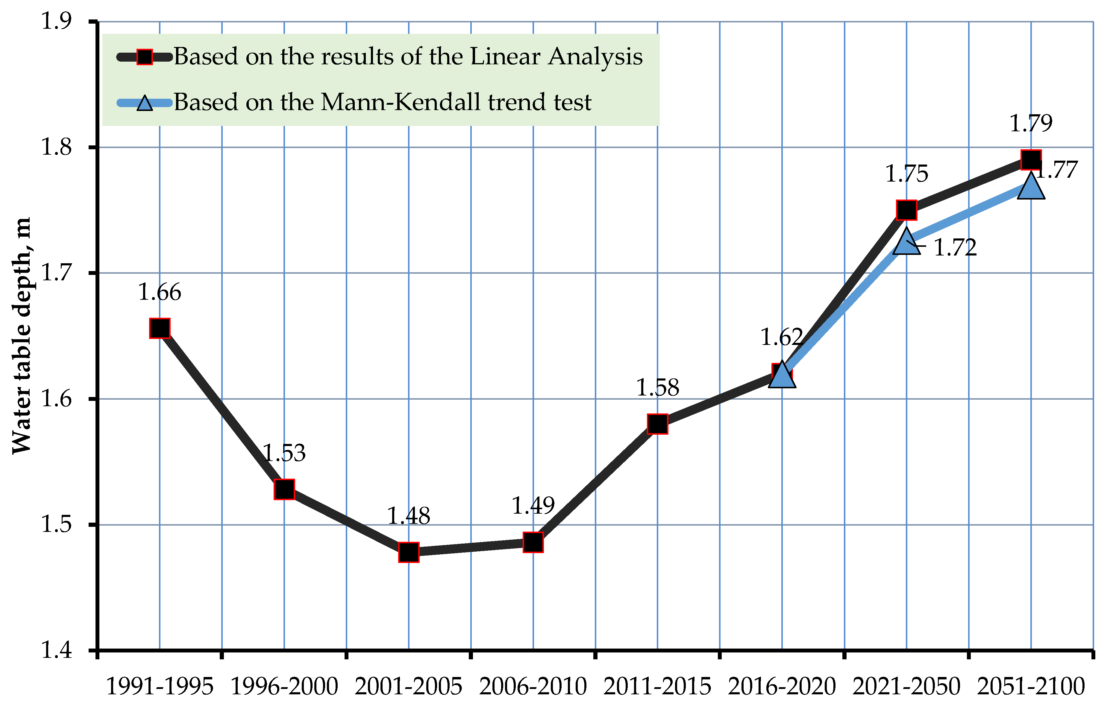
According to the results, the depth of the water table in the irrigated territories was 1.62 m, and the salinity was 1.68 g·L−1. According to the results of linear analysis, the depth will decrease to 1.75 m, and the salinity will increase to 1.97 g·L−1 by 2050. In the years 2050–2100, the water table depth is projected to be at 1.79 m and the salinity will be 2.1 g·L−1.
According to the Mann–Kendall test from 2020 to 2050, the water table depth is projected to be 1.72 m, and the salinity will be 1.72 g·L−1. In the years 2050–2100, the water table depth will be 1.77 m, and the salinity will be 1.85 g·L−1.
Across the world, the Intergovernmental Panel on Climate Change (IPCC) provides annual reports that include analyses and forecasts of climatic information based on scenarios until the end of this century. These global climate data have also been used and forecasted by the Uzbek Research Institute of Hydrometeorology. In this work, we refrained from using any scenario-based analysis and instead focused on the Mann–Kendall test and linear regression model to predict how these changes progress until the end of this century. Furthermore, the correlation accuracy between the IPCC scenarios and the results of our statistical analysis was 0.83; thus, we used statistical models.
In this study, mathematical modeling approach could also be used to have more accurate findings with regards to the impact of regional climate change on water table depth and salinity changes. However, the approach requires a complex set of comprehensive data, which will be the subject of our future research work. However, the study employed a basic mathematical approach by using the linear regression model and Mann–Kendall test.
Meanwhile, the prediction of water table depth regime involves complex solutions. It requires the study of the strength of relationship between a number of factors and the limits of this relationship. In this study, water table depth and salinity changes were averaged on a regional scale. Local level solutions could provide the accuracy of the results, which require further research. Finally, conducting water-salt balance model would provide more accurate data for salinity changes in the region. This will be studied in a future investigation.
4. Conclusions
The dynamics of the ameliorative status of irrigated lands of the Khorezm region are estimated and predicted using the linear regression model and the Mann–Kendall trend test. Based on the estimations by the linear regression model, the water table depth will be approximately 1.62 m by 2020, 1.75 m by 2050, and 1.79 m by 2100. The salinity of groundwater will be 1.68 g·L−1 by 2020, approximately 1.97 g·L−1 by 2050, and approximately 2.1 g·L−1 by 2100. Meanwhile, the Mann–Kendall trend test indicates that the water table depth will be 1.62 m by 2020, 1.72 m by 2050, and possibly 1.77 m by 2100. Moreover, the test shows that the salinity will be 1.68 g·L−1 by 2020, approximately 1.72 g·L−1 by 2050, and as high as 1.85 g·L−1 by 2100. These two approaches provided a comparison and an evaluation of the impact of climate change on groundwater in the region, and confirmed our assumptions.
Based on the above estimations, the region can expect the water table to increase in depth (although not significant depth) and increase in salinity. These results provide some clear information for policy-makers to address these potential challenges as part of ongoing and expected climate change in the region. Moreover, it is evident that irrigated lands may gradually become degraded due to salinization effects and thus, introducing modern irrigation methods to effectively use existing water resources will be essential for the region’s sustainable management of land and water resources. The ongoing implementation of water-saving irrigation technologies (such as drip and sprinkler irrigation) and the emerging water–energy–food nexus trade-offs could be potential research topics to support addressing these challenges. However, further research is needed to better explain their impacts. Additionally, the introduction of a digital agriculture concept to assess water table depth and salinity levels could provide up-to-date information about the ameliorative status of irrigated lands in the region.
Finally, it would be interesting to include more scenarios in the future (i.e., climate change with market/technology/policy changes) that may contribute to the discussion on groundwater management in the region.
Author Contributions
A.H.: Conceptualization, Methodology, Analysis, Result interpretation, Writing—editing, and Addressing comments. J.I.: Conceptualization, Methodology, Analysis, Result interpretation, and Writing—original draft preparation. M.K.: Conceptualization, Methodology, Analysis, Result interpretation, and Writing—reviewing and editing. All authors have read and agreed to the published version of the manuscript.
Funding
The study was financially supported by the Leibniz Centre for Agricultural Landscape Research (ZALF).
Acknowledgments
We would like to thank colleagues from the Tashkent Institute of Irrigation and Agricultural Mechanization Engineers (particularly Sabirjan Isaev, Bakhtiyor Matyakubov, and Kasimjan Isabaev) and the Research Institute of Irrigation and Water Problems (Ermat Shermatov) for their feedback on an earlier version of the paper. Additionally, Ahmad Hamidov’s research for this paper benefited from the German Research Foundation (DFG) within the framework of the WEFUz project (GZ: HA 8522/2-1).
Conflicts of Interest
The authors declare no conflict of interest.
References
- Hamidov, A.; Helming, K.; Balla, D. Impact of agricultural land use in Central Asia: A review. Agron. Sustain. Dev. 2016, 36, 6. [Google Scholar] [CrossRef] [Green Version]
- Unger-Shayesteh, K.; Vorogushyn, S.; Farinotti, D.; Gafurov, A.; Duethmann, D.; Mandychev, A.; Merz, B. What do we know about past changes in the water cycle of Central Asian headwaters? A review. Glob. Planet Chang. 2013, 110, 4–25. [Google Scholar] [CrossRef]
- Reyer, C.P.O.; Otto, I.M.; Adams, S.; Albrecht, T.; Baarsch, F.; Cartsburg, M.; Coumou, D.; Eden, A.; Ludi, E.; Marcus, R.; et al. Climate change impacts in Central Asia and their implications for development. Reg. Environ. Chang. 2017, 17, 1639–1650. [Google Scholar] [CrossRef]
- Jie, J.; Tianjun, Z.; Xiaolong, C.; Lixia, Z. Future changes in precipitation over Central Asia based on CMIP6 projections. Environ. Res. Lett. 2020, 15, 054009. [Google Scholar]
- Chub, V.E.; Spectorman, T.Y. Climate Trends in Uzbekistan. In Climate Change, Reasons, Impacts and Response Measures; Bulletin: Tashkent, Uzbekistan, 2016; pp. 5–16. [Google Scholar]
- Arora, N.K. Impact of climate change on agriculture production and its sustainable solutions. Environ. Sustain. 2019, 2, 95–96. [Google Scholar] [CrossRef] [Green Version]
- Musayev, S.; Musaev, I. Climate change impact on agriculture in Central Asia. Sci. -Tech. J. 2018, 22, 57–60. [Google Scholar]
- Xu, Y.; Ramanathan, V. Well below 2 °C: Mitigation strategies for avoiding dangerous to catastrophic climate changes. Proc. Natl. Acad. Sci. USA 2017, 114, 10315–10323. [Google Scholar] [CrossRef] [Green Version]
- Gruza, G.V.; Rankova, E.Y.; Aristova, L.N.; Kleschenko, L.K. On the uncertainty of some scenario climate forecasts of air temperature and precipitation in Russia. Meteorol. Hydrol. 2007, 10, 5–23. [Google Scholar]
- Israel, Y.A. An effective way to preserve climate at the present level is the main goal of solving the climate problem. Meteorol. Hydrol. 2005, 10, 5–9. [Google Scholar]
- Zhukov, V.A. Stochastic modeling and forecasting of agroclimatic resources during adaptation of agriculture to regional climate changes in Russia. Meteorol. Hydrol. 2000, 1, 100–109. [Google Scholar]
- Ivanov, V.V. Study of variations in mean monthly air temperature using sequential spectra. Meteorol. Hydrol. 2006, 5, 39–45. [Google Scholar]
- Konovalova, N.V.; Korobov, V.B.; Vasiliev, L.Y. Interpolation of climate data using GIS technology. Meteorol. Hydrol. 2006, 5, 46–53. [Google Scholar]
- Hamidov, A.; Helming, K.; Bellocchi, G.; Bojar, W.; Dalgaard, T.; Ghaley, B.B.; Hoffmann, C.; Holman, I.; Holzkämper, A.; Krzeminska, D.; et al. Impacts of climate change adaptation options on soil functions: A review of European case-studies. Land Degrad. Dev. 2018, 29, 2378–2389. [Google Scholar] [CrossRef] [PubMed]
- Huntington, T.G. Evidence for intensification of the global water cycle: Review and synthesis. J. Hydrol. 2006, 319, 83–95. [Google Scholar] [CrossRef]
- Wilby, R.L.; Whitehead, P.G.; Wade, A.J.; Butterfield, D.; Davis, R.J.; Watts, G. Integrated modelling of climate change impacts on water resources and quality in a lowland catchment: River Kennet, UK. J. Hydrol 2006, 330, 204–220. [Google Scholar] [CrossRef]
- IPCC. Climate Change 2007: The Physical Science Basis; Contribution of Working Group 1 to the Forth Assessment Report of the Intergovernmental Panel on Climate Change; Solomon, S., Qin, D., Manning, M., Chen, Z., Marquis, M., Averyt, K.B., Tignor, M., Miller, H.L., Eds.; Cambridge University Press: New York, NY, USA, 2007. [Google Scholar]
- IPCC. Summary for Policymakers. In Climate Change 2013: The Physical Science Basis; Contribution of Working Group I to the Fifth Assessment Report of the Intergovernmental Panel on Climate Change; Stocker, T.F., Qin, D., Plattner, G.-K., Tignor, M., Allen, S.K., Boschung, J., Nauels, A., Xia, Y., Bex, V., Midgley, P.M., Eds.; Cambridge University Press: Cambridge, UK; New York, NY, USA, 2013. [Google Scholar]
- Zhao, Z.; Jia, Z.; Guan, Z.; Xu, C. The Effect of Climatic and Non-climatic Factors on Groundwater Levels in the Jinghuiqu Irrigation District of the Shaanxi Province, China. Water 2019, 11, 956. [Google Scholar] [CrossRef] [Green Version]
- Gallardo, A.H. Groundwater levels under climate change in the Gnangara system, Western Australia. J. Water Clim. Chang. 2013, 4, 52–62. [Google Scholar] [CrossRef]
- Lee, J.; Jung, C.; Kim, S.; Kim, S. Assessment of Climate Change Impact on Future Groundwater-Level Behavior Using SWAT Groundwater-Consumption Function in Geum River Basin of South Korea. Water 2019, 11, 949. [Google Scholar] [CrossRef] [Green Version]
- Chung, I.-M.; Kim, J.; Lee, J.; Chang, S.W. Status of Exploitable Groundwater Estimations in Korea. J. Eng. Geol. 2015, 25, 403–412. [Google Scholar] [CrossRef] [Green Version]
- Lee, J.-Y. Lessons from three groundwater disputes in Korea: Lack of comprehensive and integrated investigation. Int. J. Water 2017, 11, 59. [Google Scholar] [CrossRef]
- Adane, Z.; Zlotnik, V.A.; Rossman, N.R.; Wang, T.; Nasta, P. Sensitivity of Potential Groundwater Recharge to Projected Climate Change Scenarios: A Site-Specific Study in the Nebraska Sand Hills, USA. Water 2019, 11, 950. [Google Scholar] [CrossRef] [Green Version]
- Terrell, B.L.; Johnson, P.N.; Segarra, E. Ogallala aquifer depletion: Economic impact on the Texas high plains. Water Policy 2002, 4, 33–46. [Google Scholar] [CrossRef]
- Scanlon, B.R.; Keese, K.E.; Flint, A.L.; Flint, L.E.; Gaye, C.B.; Edmunds, W.M.; Simmers, I. Global synthesis of groundwater recharge in semiarid and arid regions. Hydrol. Process. 2006, 20, 3335–3370. [Google Scholar] [CrossRef]
- Hamidov, A.; Beltrao, J.; Neves, A.; Khaydarova, V.; Khamidov, M. Apocynum Lancifolium and Chenopodium Album—potential species to remediate saline soils. Wseas Trans. Environ. Dev. 2007, 3, 123–128. [Google Scholar]
- Vargas, R.; Pankova, E.I.; Balyuk, S.A.; Krasilnikov, P.V.; Khasankhanova, G.M. Handbook for Saline Soil Management; FAO: Rome, Italy, 2018; p. 144. [Google Scholar]
- Global Environment Facility (GEF). The GEF Small Grants Programme. Available online: http://sgp.uz/projects/desertification/73 (accessed on 10 April 2020).
- Ishchanov, J. Analysis and Projections of the Impacts of Environmental and Climate Changes on Ameliorative Conditions of Lands in the Khorezm Region. Ph.D. Thesis, Tashkent Institute of Irrigation and Agricultural Mechnaization Engineers (TIIAME), Tashkent, Uzbekistan, 2020; p. 106. [Google Scholar]
- Ibrakhimov, M.; Maritius, C.; Lamers, J.P.A.; Tischbein, B. The dynamics of groundwater table and salinity over 17 years in Khorezm. Agric. Water Manag. 2011, 101, 52–61. [Google Scholar] [CrossRef]
- Hamidov, A.; Beltrao, J.; Costa, C.; Khaydarova, V.; Sharipova, S. Environmentally useful technique—Portulaca Oleracea golden purslane as a salt removal species. WSEAS Trans. Environ. Dev. 2007, 3, 117–122. [Google Scholar]
- Hbirkoua, C.; Martius, C.; Khamzina, A.; Lamers, J.P.A.; Welp, G.; Amelung, W. Reducing topsoil salinity and raising carbon stocks through afforestation in Khorezm, Uzbekistan. J. Arid Environ. 2011, 75, 146–155. [Google Scholar] [CrossRef]
- Devkota, M.; Gupta, R.K.; Martius, C.; Lamers, J.P.A.; Devkota, K.P.; Sayre, K.D.; Vlek, P.L.G. Soil salinity management on raised beds with different furrow irrigation modes in salt-affected lands. Agric. Water Manag. 2015, 152, 243–250. [Google Scholar] [CrossRef]
- Khamzina, A.; Lamers, J.P.A.; Martius, C.; Worbes, V.; Vlek, P.L.G. Potential of nine multipurpose tree species to reduce saline groundwater tables in the lower Amu Darya River region of Uzbekistan. Agroforest Syst 2006, 68, 151–165. [Google Scholar] [CrossRef]
- Malik, A.; Shah, A.R. Crop Production and Productivity Variations in Uzbekistan with Special Reference to Grain Crops. J. Cent. Asian Stud. 2017, 24, 121-II. [Google Scholar]
- Panda, A.; Sahu, N. Trend analysis of seasonal rainfall and temperature pattern in Kalahandi, Bolangir and Koraput districts of Odisha, India. Atmos. Sci. Lett. 2019, 20, 932. [Google Scholar] [CrossRef] [Green Version]
- Addisu, S.; Selassie, Y.G.; Fissha, G.; Gedif, B. Time series trend analysis of temperature and rainfall in lake Tana sub-basin, Ethiopia. Environ. Syst. Res. 2015, 4, 25. [Google Scholar] [CrossRef] [Green Version]
- Bhutiyani, M.R.; Kale, V.S.; Pawar, N.J. Long-term trends in maximum, minimum and mean annual air temperatures across the Northwestern Himalaya during the twentieth century. Clim. Chang. 2007, 85, 159–177. [Google Scholar] [CrossRef]
- Tabari, H.; Talaee, P. Analysis of trends in temperature data in arid and semi-arid regions of Iran. Glob. Planet. Chang. 2011, 79, 1–10. [Google Scholar] [CrossRef]
- Gil-Alana, L.A. Maximum and minimum temperatures in the United States: Time trends and persistence. Atmos. Sci. Lett. 2018, 19, 810. [Google Scholar] [CrossRef]
- Conrad, C.; Dech, S.; Dubovyk, O.; Fritsch, S.; Klein, D.; Low, F.; Zeidler, J. Derivation of temporal windows for accurate crop discrimination in heterogeneous croplands of Uzbekistan using multitemporal Rapid Eye images. Comput. Electron. Agric. 2014, 103, 63–74. [Google Scholar] [CrossRef]
- Djumaboev, K.; Hamidov, A.; Anarbekov, O.; Gafurov, Z.; Tussupova, K. Impact of institutional change on irrigation management: A case study from southern Uzbekistan. Water 2017, 9, 419. [Google Scholar] [CrossRef] [Green Version]
- Simonett, O.; Novikov, V. Land Degradation and Desertification in Central Asia: Central Asian Countries Initiative for Land Management, Analysis of the current state and recommendation for the future. Zoï Environ. Netw. Swiss Gef Counc. Memb. Geneva 2010, 1–19. [Google Scholar]
- Uzbekistan State Committee. Urban and Rural Population by Regions for 2017. Available online: https://www.stat.uz/uz/statinfo/demografiya-va-mehnat/statistik-jadvallar-demografiya/220-ofytsyalnaia-statystyka-uz/demografiya-i-trud-uz/demograficheskie-pokazateli-uz/2399-hududlar-bo-yicha-shahar-va-qishloq-aholisi-soni-yil-boshiga-ming-kishi (accessed on 1 May 2020).
- Hamidov, A.; Kasymov, U.; Salokhiddinov, A.; Khamidov, M. How can intentionality and path dependence explain change in water-management institutions in Uzbekistan? Int. J. Commons 2020, 14, 16–29. [Google Scholar] [CrossRef] [Green Version]
- Yan, X.; Su, X. Linear Regression Analysis: Theory and Computing; World Scientific Publishing: Hackensack, NJ, USA, 2009; p. 348. [Google Scholar]
- Warne, R.T. Beyond multiple regression: Using commonality analysis to better understand R2 results. Gift. Child Q. 2011, 55, 313–318. [Google Scholar] [CrossRef]
- Ratner, B. The correlation coefficient: Its values range between +1/−1, or do they? J. Target. Meas. Anal. Mark. 2009, 17, 139–142. [Google Scholar] [CrossRef] [Green Version]
- Lakin, G.F. Biometrics, 4th ed.; Higher School: Moscow, Russia, 1990; p. 352. [Google Scholar]
- Patle, G.T.; Singh, D.K.; Sarangi, A.; Rai, A.; Khanna, M.; Sahoo, R.N. Time series analysis of groundwater levels and projection of future trend. J. Geol. Soc. India 2015, 2, 232–242. [Google Scholar] [CrossRef]
- Allen, D.M. Historical trends and future projections of groundwater levels and recharge in costal British Columbia, Canada. In Proceedings of the SWIM 21-21st Salt Water Intrusion meeting 2010, Azores, Portugal, 21–26 June 2010; pp. 267–270. [Google Scholar]
- Chaudhuri, S.; Dutta, D. Mann–Kendall trend of pollutants, temperature and humidity over an urban station of India with forecast verification using different ARIMA models. Environ. Monit. Assess. 2014, 186, 4719–4742. [Google Scholar] [CrossRef] [PubMed]
- Emami, F.; Masiol, M.; Hopke, P.K. Air pollution at Rochester, NY: Long-term trends and multivariate analysis of upwind SO2 source impacts. Sci. Total Environ. 2018, 612, 1506–1515. [Google Scholar] [CrossRef] [PubMed]
- Ma, J.; Hung, H.; Tian, C.; Kallenborn, R. Revolatilization of persistent organic pollutants in the Arctic induced by climate change. Nat. Clim. Chang. 2011, 1, 255–260. [Google Scholar] [CrossRef] [Green Version]
- Vanguelova, E.I.; Benham, S.; Pitman, R.; Moffat, A.J.; Broadmeadow, M.; Nisbet, T.; Durrant, D.; Barsoum, N.; Wilkinson, M.; Bochereau, F.; et al. Chemical fluxes in time through forest ecosystems in the UK–soil response to pollution recovery. Environ. Pollut. 2010, 158, 1857–1869. [Google Scholar] [CrossRef] [PubMed]
- Mann, H.B. Nonparametric tests against trend. Econometrica 1945, 13, 245–259. [Google Scholar] [CrossRef]
- Kendall, M.G. Rank Correlation Methods; Griffin: London, UK, 1975. [Google Scholar]
- Jaiswal, A.; Samuel, C.; Kadabgaon, V.M. Statistical trend analysis and forecast modeling of air pollutants. Glob. J. Environ. Sci. 2018, 4, 427–438. [Google Scholar]
- Hirsch, R.M.; Slack, J.R. A Nonparametric Trend Test for Seasonal Data with Serial Dependence. Water Resour. Res. 1984, 20, 727–732. [Google Scholar] [CrossRef] [Green Version]
- Panda, D.K.; Mishra, A.; Kumar, A. Quantification of trends in groundwater levels of Gujarat in western India. Hydrol. Sci. J. 2012, 7, 1325–1336. [Google Scholar] [CrossRef]
- Biswas, B.; Jain, S.; Rawat, S. Spatio-temporal analysis of groundwater levels and projection of future trend of Agra city, Uttar Pradesh, India. Arab. J. Geosci. 2018, 11, 278. [Google Scholar] [CrossRef]
- Conrad, C.; Schorcht, G.; Tischbein, B.; Davletov, S.; Sultonov, M.; Lamers, J.P.A. Agro-Meteorological Trends of Recent Climate Development in Khorezm and Implications for Crop Production; Martius, C., Rudenko, I., Lamers, J.P.A., Vlek, P.L.G., Eds.; Cotton, Water, Salts and Soums—Economic and Ecological Restructuring in Khorezm, Uzbekistan; Springer: Berlin, Germany, 2012; pp. 25–36. [Google Scholar]
- Qian, C.; Zhang, X.; Li, Z. Linear trends in temperature extremes in China, with an emphasis on non-Gaussian and serially dependent characteristics. Clim. Dyn. 2019, 53, 533–550. [Google Scholar] [CrossRef] [Green Version]
- Nazir Zaz, S.; Ahmad Romshoo, S.; Thokuluwa Krishnamoorthy, R.; Viswanadhapalli, Y. Analyses of temperature and precipitation in the Indian Jammu and Kashmir region for the 1980-2016 period: Implications for remote influence and extreme events. Atmos. Chem. Phys. 2019, 19, 15–37. [Google Scholar]
- He, M.; Russo, M.; Anderson, M.; Fickenscher, P.; Whitin, B.; Schwarz, A.; Lynn, E. Changes in extremes of temperature, precipitation, and Runoff in California’s Central Valley During 1949–2010. Hydrology 2018, 5, 1. [Google Scholar] [CrossRef] [Green Version]
Figure 1.
Map of the Khorezm region, Uzbekistan.

Figure 2.
Average annual temperature at the Khiva weather station from 1928 to 2017.

Figure 3.
Water table depths and salinity in the Khorezm region during 1991–2017.

Figure 4.
Predictions of groundwater salinity.

Figure 5.
Predictions of water table depth.


Table 1.
Average annual air temperature at the Khiva weather station for 1928–2017.
| Variable | Number of Years | Minimum | Maximum | Mean | Standard Deviation |
|---|---|---|---|---|---|
| Average annual air temperature | 90 | 10.558 | 14.983 | 12.961 | 1.020 |
Table 2.
Sen’s slope of all meteorological parameters.
| Sen’s Slope | Air Temperature | Absolute Humidity, mm | Relative Humidity, % | Land Surface Temperature | Precipitation, mm | Wind Speed, m·s−1 | ||||
|---|---|---|---|---|---|---|---|---|---|---|
| Mean | Max | Min | Mean | Max | Min | |||||
| Period = 10 years | 0.284 | 0.246 | 0.423 | 0.252 | 0.451 | 0.506 | −0.708 | 0.17 | −0.617 | −0.224 |
© 2020 by the authors. Licensee MDPI, Basel, Switzerland. This article is an open access article distributed under the terms and conditions of the Creative Commons Attribution (CC BY) license (http://creativecommons.org/licenses/by/4.0/).
Share and Cite
MDPI and ACS Style
Hamidov, A.; Khamidov, M.; Ishchanov, J. Impact of Climate Change on Groundwater Management in the Northwestern Part of Uzbekistan. Agronomy 2020, 10, 1173. https://doi.org/10.3390/agronomy10081173
AMA Style
Hamidov A, Khamidov M, Ishchanov J. Impact of Climate Change on Groundwater Management in the Northwestern Part of Uzbekistan. Agronomy. 2020; 10(8):1173. https://doi.org/10.3390/agronomy10081173
Chicago/Turabian StyleHamidov, Ahmad, Mukhamadkhan Khamidov, and Javlonbek Ishchanov. 2020. "Impact of Climate Change on Groundwater Management in the Northwestern Part of Uzbekistan" Agronomy 10, no. 8: 1173. https://doi.org/10.3390/agronomy10081173
Note that from the first issue of 2016, this journal uses article numbers instead of page numbers. See further details here.