

Abstract
Topographically delineated catchments are the common spatial unit to connect human activities and climate change with their consequences for water availability as a prerequisite for sustainable water management. However, inter-catchment groundwater flow and limited connectivity within the catchment results in effective catchment areas different from those suggested by surface topography. Here, we introduce the notion of effective catchment area quantified through an effective catchment index (ECI), derived from observed streamflow, precipitation and actual evapotranspiration estimates, to understand the prevalence and significance of substantial differences between topographic and effective catchment areas in a global dataset. We evaluate our ECI analysis by comparing it to hydraulic head simulations of a global groundwater flow model and to the Budyko framework. We find that one in three studied catchments exhibit an effective catchment area either larger than double or smaller than half of their topographic area. These catchments will likely be affected by management activities such as groundwater pumping or land use change outside their topographic boundaries. Or alternatively, they affect water resources beyond their topographic boundaries. We find that the magnitude of the observed differences is strongly linked to aridity, mean slope, distance to coast, and topographic area. Our study provides a first-order identification of catchments where additional in-depth analysis of subsurface connectivity is needed to support sustainable water management.
Export citation and abstract BibTeX RIS

Original content from this work may be used under the terms of the Creative Commons Attribution 4.0 license. Any further distribution of this work must maintain attribution to the author(s) and the title of the work, journal citation and DOI.
1. Introduction
Sustainable water resources management requires a robust understanding of the connection between management activities and their consequences for freshwater availability. Traditional water management has focused on what is sometimes called blue water, i.e. water available for development and supply through pumping (groundwater) or the creation of artificial reservoirs (mainly through the damming of rivers). This view has been expanded to include activities that influence green water (soil moisture, Falkenmark and Rockström 2006), such as land use change which partially controls the amount of soil moisture removed from the terrestrial water cycle through evapotranspiration (Gordon et al 2005, Schewe et al 2019). Blue and green water availability is often quantified using discharge observations at the outlet of topographically delineated catchments, driven by climatic forcing and assuming a closed water balance. For this reason, topographic catchments are deemed the basic unit for water management activities and they represent a common scale for hydrologic research and practice (Wagener et al 2007). Consequently, a growing number of hydro-meteorological catchment scale datasets have been developed to enable hydrologic analysis and advance understanding (Duan et al 2006, Addor et al 2017).
However, regional groundwater flow systems can remove water from or add water to topographic catchments (Tóth 1962), resulting in a violation of the assumption of a closed water balance. Such groundwater connectivity means that some catchments collect water from areas beyond their topographic boundaries, while others are effectively much smaller than their surface topography suggests. Evidence for this problem comes so far from studies of individual catchments or from those performed in geographically-focused regions (e.g. Le Moine et al 2007, Schaller and Fan 2009, Muñoz et al 2016, Fan 2019), and a wider discussion of the consequences for water management activities is still missing. In hydrologic research and practice, most modeling strategies currently ignore the consideration of groundwater connectivity assuming that catchments are not connected to their surroundings (Bouaziz et al 2018). So far, no global analysis of this problem has been performed and the conditions that control the extend of this problem are still largely unexplored.
In this study, we introduce the notion of effective catchment area and define a novel metric, the Effective Catchment Index (ECI), to detect and quantify differences between topographic and effective catchment areas. We determine ECI for a global set of catchments derived from various publicly available datasets and use a random forest to understand controls on its magnitude.
2. Materials and methods
2.1. The effective catchment index (ECI)
We define a new metric, the ECI, to describe the deviation of the effective catchment area from the topographic catchment area. It is an evolution of the discharge/recharge ratio introduced by Schaller and Fan (2009) and adds the following advantages: (i) the sign of ECI indicates whether a catchment is gaining water (+) or losing water (-); and (ii) the absolute value of ECI indicates the strength of water gains and losses. Catchments with similar absolute values but different signs of ECI have the same relative influence of water gains or losses. ECI enables us to estimate the effective area of a catchment in contrast to its topographic area and to quantify inter-catchment groundwater flow. It is calculated as follows:
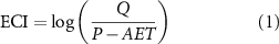
where Q [mm/d] is the long-term observed average specific streamflow at the catchment outlet (volumetric flow rate normalized by topographic catchment area). P [mm/d] and AET [mm/d] are long-term average estimates of precipitation and actual evapotranspiration, respectively (see section 2.2). For ECI > 0: catchments gain water, i.e. their effective area is larger than their topographic area; for ECI < 0: catchments lose water, i.e. their effective area is smaller than their topographic area.
Assuming the presence of inter-catchment groundwater flow (±IGF), the continuity equation can be defined by dS/dt = P-AET-Q + IGF, where dS/dt is the change of storage. Assuming further that the long-term water balance has similar starting and ending storage conditions, the influence of storage becomes negligible (dS/dt ≅ 0). We can then quantify the relationship between P-AET and Q using ECI, which quantifies the significance of IGF. The observed mean discharge at the catchment outlet, Q, represents the response of the effective catchment ( [km2]), while the difference of catchment average precipitation (P) and actual evapotranspiration (AET), P-AET, represents the response of the topographic catchment (
 [km2]). Therefore, the ratio of the effective to the topographic catchment area (
 ) can be calculated as follows:
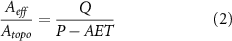
Combing equations (1) and (2) yields:
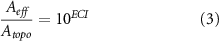
where the uncertainty in estimates of this ratio is considered with the uncertainty in the ECI estimates (see section 2.3).
2.2. Data
In our study, discharge observations are obtained from several sources (table 1) described in detail by Beck et al (2019a). Based on the best availability of discharge observations, we choose the 10-year time period 2000–2009 to calculate long-term averages of ECI. We further selected precipitation and actual evapotranspiration datasets according to the following quality criteria (i) temporal coverage: the precipitation and actual evapotranspiration datasets should cover the time period 2000–2009 to coincide with good discharge availability; (ii) the spatial resolution should not be coarser than around 0.25° × 0.25°, because forcing with too coarse a resolution may result in unexpected uncertainty for small catchments due to the averaging over a large area. Based on these criteria, three independent precipitation and three independent actual evapotranspiration products were deemed suitable to perform our analysis (table 1).
Table 1. Datasets of discharge, precipitation, and actual evapotranspiration that are used to calculate ECI.
| Producta | Temporal resolution | Spatial resolution (Lat × Lon) | Reference | |
|---|---|---|---|---|
| Discharge Q | USGS-NWIS, GAGES-II, GRDC, HidroWeb-snirh, EWA of EURO-FRIEND-Water, CCM2-JRC CCM, WSC-HYDAT, BoM, CR2 and CAMELS-CL | Daily | – | Beck et al 2019a |
| Precipitation P | MSWEP v2.2 | Daily | 0.1° × 0.1° | Beck et al 2019b |
| ERA5 | Monthly | 0.25° × 0.25° | Hersbach et al 2018 | |
| GLDAS | Daily | 0.25° × 0.25° | Li et al 2018, Rodell et al 2004 | |
| Actual evapotranspiration AET | GLEAM | Daily | 0.25° × 0.25° | Martens et al 2017, Miralles et al 2011 |
| MODIS | Annual | 0.0083° × 0.0083° | Zhao et al 2006 | |
| CMIP6 | Monthly | 0.2347° × 0.3125° | Scoccimarro et al 2017 |
aUSGS-NWIS: United States Geological Survey (USGS) National Water Information System (NWIS), GRDC: the Global Runoff Data Centre, HidroWeb-snirh: the HidroWeb portal of the Brazilian Agência Nacional de Águas, EWA: the European Water Archive, CCM2-JRC CCM: CCM2-JRC CCM River and Catchment Database, WSC-HYDAT: Water Survey of Canada (WSC) National Water Data Archive (HYDAT), BoM: the Australian Bureau of Meteorology, CR2: the Chilean Center for Climate and Resilience Research.
Topographic areas of our analyzed catchments are in the range of 1 − 50 000 km2. The majority (85%) of those are larger than 100 km2, and 46% are larger than 625 km2 (which is approximately 0.25° × 0.25°). The distribution of catchment topographic areas is provided in figure S1 (available online at stacks.iop.org/ERL/15/104024/mmedia). To further minimize the influence of irrigation on ECI estimates, we only consider catchments (table 1) with irrigation areas < 5% of the total catchment area. By doing so we exclude the influence of pumping to a large extent, even though pumping might still occur for other purposes than irrigation, which would not be captured by our analysis (see figure S3). These considerations result in a final catchment set of 8701 catchments for analysis.
2.3. Conclusive catchments and consideration of ECI uncertainty
Uncertainty in the ECI calculation originates from uncertainties in the discharge, precipitation, and actual evapotranspiration datasets. Compared to the precipitation and actual evapotranspiration datasets, discharge observations are assumed to contain much smaller uncertainty (Sauer and Meyer 1992, Biemans et al 2009, Khan et al 2018). We therefore focus on the uncertainties introduced through the precipitation and actual evapotranspiration data, by analyzing the range of ECI estimates obtained from the nine possible combinations of the three independent actual evapotranspiration and the three independent precipitation datasets (table 1). We define 'conclusive' catchments as those where at least seven out of nine possible ECI estimates can be calculated (given that some datasets do not cover all catchments) and that these have the same ECI sign (effective catchment areas are therefore either all larger than or all smaller than the corresponding topographic catchment areas). We subsequently use the mean of the conclusive ECI estimates for further analysis. We show in the supplemental material (figure S2) that the variability across the forcing data products is not higher for small catchments than it is for large ones. Thus providing at least some evidence that data bias related to poorer estimates over smaller areas is not causing the ECI results. Results using more stringent criteria are shown in the supplemental material. Adopting those would not change our overall conclusions.
2.4. Identification of influencing factors
We use a random forest analysis to identify and rank the most relevant factors influencing the variability of ECI (Breiman 2001). Random forest is an tree-based ensemble learning method for classification and regression (Denisko and Hoffman 2018), which has been widely applied to identify the most 'important' factors that organize a dataset (Tyralis et al 2019). Building on the idea of hydrologic landscapes with respect to expected dominant controls on the water balance (Winter 2001), we use physiographic factors (Beck et al 2015) that characterize a catchment's climate, topography, and geology, while adding aspects of catchment location: aridity index (AI), distance to the coast (D), topographic catchment area (A), mean slope (S), permeability (µ), and mean elevation (H). In addition, the fraction of lakes and reservoirs (fw) is considered. We apply a 10-fold cross-validation and use different numbers of ensembles (50, 100, and 200) to control the quality of the regression trees. We identify the most relevant factors using importance estimates derived from permutations of the out-of-bag predictor observations of the random forest. To avoid false conclusions due to the pre-selection of conclusive catchments (see section 2.3), we also apply the random forest analysis to the 2760 conclusive catchments as well as to all 8701 catchments. Random forest analyses using different numbers of ensembles demonstrate similar results of the importance ranking for all influencing factors. Therefore, we only show the importance estimates derived from the random forest analysis using 200 ensembles.
2.5. Evaluation of ECI estimates
We evaluate our ECI estimates for the conclusive catchments in two independent ways. First, we assess the consistency of water gains or losses (the direction of inter-catchment groundwater flow) indicated by our ECI values and those indicated by an independently simulated hydraulic gradient. We use hydraulic head simulations of a steady-state global groundwater model with a spatial resolution of around 9 × 9 km2 at the equator (Reinecke et al 2019b). We define buffer areas inside and outside of the catchment boundary to estimate the average value of all head estimates that fall inside these buffer areas. Then, comparing the mean hydraulic head of the two buffer areas that are inside (hin) and outside (hout) of the catchment boundary, we obtain the head difference across the catchment boundary Δhsim = hin-hout. This head difference can be used to indicate the direction of inter-catchment groundwater flow (positive or negative ECI). However, estimating actual groundwater fluxes at the catchment boundaries is complicated and requires good knowledge of subsurface properties, which we do not have for all these catchments. Therefore, we only evaluate the direction of water flux using the head simulations. We make the simple assumption that a positive head difference (Δhsim > 0) indicates a losing catchment (ECI < 0), while a negative head difference (Δhsim < 0) indicates a gaining catchment (ECI > 0). Due to the spatial resolution of the available head simulations, the calculation of head differences for smaller catchments may not be possible when an insufficient number of head simulations fall within the buffer areas. To not exclude too many catchments in the evaluation, we test different buffer areas with 20%, 30% and 40% of the topographic catchment area. With these three fractions, the mean hydraulic head of the buffer areas can be derived for 70%, 78% and 81% of the conclusive catchments, respectively. We use the buffer area of 30% of the topographic catchment area for the ECI evaluation below. Evaluations using the other two areas show similar results (see section 7 of the supplemental material).
Second, we identify outliers from the expected range of the Budyko curve (Budyko et al 1974). These outliers may be caused by problems with the water balance (Le Moine et al 2007, Bouaziz et al 2018). We therefore evaluate the consistency of our ECI estimates with the outliers in the Budyko framework. We plot the relationship between the long-term dryness index PET/P and the long-term evaporative index (P-Q)/P (figure 4). Using P-Q instead of AET is beneficial to detect the unrealistic water balance values. PET is obtained from the GLEAM dataset (Miralles et al 2011, Martens et al 2017). P is the mean of the three precipitation products (table 1). We adopt the widely used Fu (1981) curve (equation (4)) to represent the Budyko curve, which is identical to the Fu curve with w = 2.6 (Beck et al 2019a). We show a feasible range around the Budyko curve using two other Fu curves with w = 1.8 and w = 3.8, which indicate the 90% confidence interval of the w parameter derived from a set of 411 MOPEX catchments (Greve et al 2015).
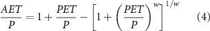
where w [-] is an empirical parameter that represents catchment characteristics.
A catchment with a closed water balance cannot discharge or evaporate more water than it receives as precipitation (over longer time periods), and actual evapotranspiration cannot be larger than potential evapotranspiration due to the energy limit (Bouaziz et al 2018). Therefore, assuming negligible observational error, this suggests that a catchment with Q > P (area below x-axis in figure 4) gains water (ECI > 0), and that a catchment with P-Q > PET (areas above the energy limit in figure 4) loses water (ECI < 0) through the subsurface. Bouaziz et al (2018) further postulate that catchments that plot further away from the theoretical relationship between dryness and evaporative index are more likely impacted by groundwater gains or losses. We would therefore expect that ECI values should grow (either negatively or positively) with increasing distance from the theoretical relationship.
3. Results and discussion
3.1. Global distribution of ECI
Through the analysis of the 2760 conclusive catchments (figure 1), we find that substantial deviations between topographic and effective catchment areas are abundant across the globe (circles in dark red and dark blue in figure 1). We define substantial as: the effective areas are either larger than double or smaller than half of their corresponding topographic catchment areas. About 36% of the conclusive catchments show such a substantial deviation. Consequently, blue water availability in these catchments will likely be affected by management activities outside their topographic boundaries, or, activities within topographic boundaries will affect water resources outside.

Figure 1. Global distribution of ECI. Colored circles represent 2760 conclusive catchments from the 8701 catchments, while the grey squares indicate inconclusive catchments. The dark blue and dark red circles represent catchments with the effective area that is either more than double or smaller than half of the topographic area. The light blue and light red circles indicate catchments with a smaller deviation between the topographic and effective catchment areas compared to the circles in dark blue and dark red.
Download figure:
Standard image High-resolution imageIn North America, our analysis indicates that 2117 of 6172 (∼34%) catchments are conclusive. Among those, 691 catchments show substantial deviations between effective and topographic catchment areas. In the US, our analysis demonstrates that catchments located in the Upper Mississippi River Basin gain water from neighboring areas resulting in larger effective catchment areas (positive ECI, blue circles). While catchments in the Colorado River Basin show smaller effective catchment areas (negative ECI, red circles), indicating losing water conditions. These results agree well with a previous regional study on groundwater exporters and importers in the US (Schaller and Fan 2009). Additionally, many costal catchments in Southern California show smaller effective catchment areas (negative ECI), which suggests that these catchments export water to the North Pacific Ocean via submarine groundwater flow (Luijendijk et al 2020). In Europe, 212 of 629 (∼34%) catchments are identified as conclusive catchments, 43 of which have substantial differences between effective and topographic catchment areas. The result is consistent with a modeling study of a large sample of catchments in France (Le Moine et al 2007), which showed that explicitly representing inter-catchment groundwater transfers is preferable to address the water balance issues in rainfall-runoff models. In Australia, we find that 82 of the 89 conclusive catchments are costal catchments with losing water conditions (negative ECI). 80% of these coastal losing catchments are also in arid regions (PET/P > 1), which suggests the importance of inter-catchment groundwater flow in the coastal and arid areas of Australia.
Repeating the analysis with a requirement that at least eight out of nine or all nine ECI estimates are consistent (to test the robustness of our results), produces 30% (2573) and 28% (2442) conclusive catchments, respectively. There is therefore no significant impact on our conclusions using more stringent criteria (figures S4 and S5). However, our analysis, similar to others done previously (Bouaziz et al 2018), assumes that observational errors are negligible (as long as the independent datasets are consistent). We could in contrast assume that subsurface groundwater interactions are negligible, and that precipitation bias is the only relevant factor—the opposite extreme. Under this assumption, Beck et al (2019a) showed that precipitation in mountain ranges may be underestimated, which would be consistent with widely made assumptions about the quality of precipitation measurements in mountainous regions. The truth likely lies in-between the two assumptions of no-groundwater interactions and perfect precipitation measurements—both are unlikely to be true in most places and it is rather a question of dominance. Further insights will have to come from additional local analyses where additional information on data quality, geological settings etc is available (Le Moine et al 2007, Muñoz et al 2016).
3.2. Identifying important influencing factors
The random forest prediction of ECI values shows consistent results concerning the relative importance of all the influencing factors for all 8701 catchments and for the 2760 conclusive catchments (figure 2). By quantifying the permutation importance estimates of all seven factors that represent a catchment's climate, topography, geology, and location (figure 2), we find that aridity index is by far the strongest influencing factor, followed by mean slope, distance to coast, topographic catchment area, permeability, fraction of lakes and reservoirs, and mean elevation. We, therefore, analyze the relationship between ECI and the most relevant influencing factors in more detail (see section 3.3), i.e. aridity index, mean slope, distance to coast, and topographic catchment area.

Figure 2. Importance estimates of the ECI influencing factors for the 2760 conclusive and 8701 entire catchments.
Download figure:
Standard image High-resolution image3.3. Factors influencing ECI
For the 2760 conclusive catchments, 17% of ECI values indicate that the effective catchment area is smaller than half of their topographic area, while 19% show that the effective catchment area is larger than double of that suggested by topography (figure 3(a)). Analyzing the relationship between ECI and the four most important influencing factors for the 2760 conclusive catchments, we find that more arid catchments tend to lose more water, which results in smaller effective catchment areas (figure 3(b)). In wetter regions, the other influencing factors, beyond AI, gain more importance. This is in line with the numerical model simulations in a drier climate by Schaller and Fan (2009), who showed that in arid regions the regional groundwater table often falls below stream beds and much of the recharge through local precipitation enters the regional groundwater flow system rather than the river. A decreasing trend in ECI is found with decreasing distance to the coast (figure 3(c)), suggesting that near-coast catchments tend to lose water through subsurface drainage to the sea. This result is consistent with previous studies on submarine groundwater discharge in coastal catchments, which showed that submarine groundwater discharge can be as important as surface river discharge entering the Atlantic Ocean (Moore et al 2008). ECI variability also decreases with increasing slope (figure 3(d)) and increasing catchment area (figure 3(e)), indicating a higher variability of effective catchment area in flatter regions and for smaller catchments. Consequently, it shows smaller deviations for large basins, which one would expect since their areas should be more consistent with regional groundwater systems. There is some statistical dependency between the four influencing factors (figure S6), which can be explained by physiography. For instance, aridity index is positively correlated with distance to the coast since inland regions in general are more likely to be arid than coastal regions (Makarieva et al 2009, Trenberth et al 2011). The relationships between ECI and the influencing factors do not change substantially when using at least eight out of nine or all nine ECI estimates to define conclusive catchments (figures S7 and S8).

Figure 3. (a) Distribution of the ratio of effective catchment area to topographic catchment area; relationships between Effective Catchment Index (ECI) estimates and (b) aridity index, (c) distance to the coast, (d) mean slope, and (e) topographic catchment area. Since no clear patterns are found for the other influencing factors, we show the relationship between ECI and the most relevant influencing factors (b − e). Colored circles indicate conclusive catchments, while the grey squares indicate inconclusive catchments. The grey dashed lines indicate effective catchment areas being either more than double or less than half of topographic catchment areas, respectively. The aridity index represents the long-term ratio of potential evapotranspiration to precipitation. Distance to the coast is calculated as the shortest distance (as the crow flies) between the catchment centroid and the coast. Aeff and Atopo represent the effective and topographic catchment areas, respectively.
Download figure:
Standard image High-resolution image
Figure 4. Evaluation using Budyko framework. Blue dashed lines show the water limit, and the red dashed line indicates the energy limit. Black solid line shows the Fu curve with w = 2.6, which is identical to the Budyko curve (Budyko et al 1974). Two black dashed lines show a feasible range around the Budyko curve using the 90% confidence interval of w parameter from Greve et al (2015). Blue and red circles indicate conclusive catchments with ECI > 0 and ECI < 0, respectively.
Download figure:
Standard image High-resolution image
3.4. Assessing the consistency of ECI with other strategies
We compare the direction of inter-catchment groundwater flow (water gains or losses) based on our ECI estimates with that derived from the simulated head differences to assess the consistency between the two approaches. For gaining catchments, we find an increasing agreement with simulated head differences for increasing ECI values (figure S9(a)). When ECI > 0.3, more than half of the conclusive catchments show a consistent direction of water gains or losses compared to the groundwater model. With increasing ECI values, the percentage of the consistent catchments between our results and the groundwater model can become greater than 70%. We find a similar pattern for losing catchments (figure S9(b)), with an increasing percentage of consistency when ECI values become more negative. The percentage of consistent catchments can reach up to 80% for strongly negative ECI values. Results are robust when we use different buffer areas to calculate the head differences (figure S9). We would not expect a full agreement between our ECI estimates and the groundwater model due to reasons such as uncertainties in the forcing data that are used to derive ECI and in the groundwater flow simulations, and the steady-state assumption of the groundwater model. However, we expect the high agreement between the two approaches for catchments with significant water gains or losses (those with large positive or negative ECI values), which is indeed showed with the comparison between ECI estimates and the groundwater model. The impacts of uncertainties in both forcing data and head simulations (Reinecke et al 2019b) are likely more pronounced for catchments with smaller absolute ECI values. Furthermore, subsurface heterogeneity, subsurface conductivity and resolution of the groundwater model used will affect our evaluation (Reinecke et al 2019a, 2020). More detailed subsurface conceptualizations and subsequent higher resolution groundwater modeling would be required to resolve these issues.
Inter-catchment groundwater flow leads to a violation of the assumption of a closed water balance for topographic catchments. Catchments with significant inter-catchment flow are therefore expected to deviate from the theoretical relationship defined by Budyko and discussed in section 2.5 (Budyko, 1974; Bouaziz et al 2018). We therefore expect larger deviations from the Budyko curve for catchments with larger absolute values of ECI. Indeed, we find that conclusive catchments with higher water gains or losses (dark blue and dark red circles) deviate more from the Budyko curve (figure 4). This general similar pattern is still largely preserved for the inconclusive catchments (figure S10). We thus find a consistency between the Budyko framework and the water gains/losses identified by ECI. We further divide figure 4 into three zones to discuss the outliers present. (i) An area that is above the energy limit (Zone 1). In this zone, the calculated AET, derived using P-Q, is larger than PET. Due to the limited energy available, AET cannot be larger than PET for catchment with a closed water balance. However, for losing catchments we may wrongly attribute water loss to AET under the assumption of a closed water balance. Indeed, we find a large portion of losing catchments (red circles) identified by ECI are located within this zone. (ii) An area with (P-Q)/P < 0 (below the lower blue dashed line) represents a second water limit (Zone 2). The area above the water limit with Q = 0 (upper blue dashed line) shows that discharge cannot become negative. Whereas, the zone below the water limit with Q = P (lower blue dashed line) shows that specific discharge Q can be larger than P for the topographic catchment. Since Q cannot be larger than P considering a closed water balance, catchments within this zone can be assumed to gain water from outside the topographic catchment boundary. We see that many gaining catchments (blue circles) identified by ECI fall within this zone. (iii) An area that is between the energy limit and the two water limits (Zone 3). In this zone, we find that many losing catchments (red circles) are above the Budyko range, while the gaining catchments (blue circles) are mostly located below the Budyko range. Therefore, inter-catchment groundwater flow could be one likely reason for catchments that are located outside this feasible Budyko range. However, the deviation of catchments from the Budyko curve may also be affected by other factors, such as P and PET seasonality, P phase, vegetation cover, soil moisture capacity, and topography (Beck et al 2019a). Generally, the analysis of Budyko framework helps us to explain a large proportion of gaining and losing catchments identified by ECI.
4. Conclusions
We define a new metric, the ECI, to reveal the occurrence and strength of gaining or losing groundwater conditions for topographically delineated catchments. This ECI detects and quantifies differences between effective and topographic catchment areas. Our analysis with this index provides evidence that the assumption of a closed water balance in topographic catchments does not hold for a substantial number of catchments across the globe. One in three studied catchments have an effective catchment area that is even larger than double or smaller than half of their topographic catchment area. Consequently, these catchments will potentially be affected by water management activities such as groundwater pumping, as well as land management activities such as deforestation or reforestation, outside their topographic boundaries. Similarly, activities within their topographic boundaries might affect blue water resources outside. This result provides further indication that studies ignoring the inter-catchment groundwater flow may draw conclusions biased by a false assumption of a closed water balance for their topographic catchments. Our ECI analysis is largely consistent with hydraulic head simulations derived using a global groundwater flow model, as well as with expectations derived from the Budyko framework. Our newly defined ECI provides a simple and easily applied diagnostic tool to account for the deviations between effective and topographic catchments. This index can be used in hydrological modeling studies to estimate effective catchment areas, in drought analysis to study the enhancement of drought propagation due to inter-catchment groundwater flow, and in the analysis of climate and land use change impacts on cross-boundary water exchange. Thus, it provides the first step towards better understanding the hydrologically effective area of catchments and provides first-order insight where additional in-depth analysis of subsurface connectivity across topographic boundaries is needed to support sustainable water management. Further study is needed to include geological information into the analysis so that the spatial extend and subsurface connectivity of the effective catchment can be defined.
Acknowledgments
We thank Kevin McGuire for reference suggestions. We thank Robert Reinecke for the discussion about his groundwater model. YL and AH were supported by the Emmy-Noether-Programme of the German Research Foundation (DFG, Grant Nos. HA 8113/1-1). TW was partially supported by a Royal Society Wolfson Research Merit Award (WM170042). HB was partially supported by the U.S. Army Corps of Engineers' International Center for Integrated Water Resources Management (ICIWaRM). The Global Runoff Data Centre (GRDC) is thanked for providing part of the streamflow data. We also thank Tanja de Boer-Euser and one anonymous reviewer for their constructive comments. The article processing charge was funded by the University of Freiburg in the funding programme Open Access Publishing.
Data availability statement
The data that support the findings of this study are available upon reasonable request from the authors.