Pre-Selection of the Optimal Sitting of Phase-Shifting Transformers Based on an Optimization Problem Solved within a Coordinated Cross-Border Congestion Management Process

Abstract

The current European policy roadmap aims at forcing the TSOs to coordinate remedial actions used for relieving the congestions in the synchronous power system. In this paper, an optimization problem for coordinated congestion management is described and its results obtained for a real European use cases created in the H2020 EU-SysFlex project are presented. First of all, these results prove the feasibility of a central optimization problem for the coordination of the cross-border congestion management process. Next, the formulated optimization problem is used to tackle the issue of planning the investments in phase-shifting transformers (PSTs), for the purpose of increasing the efficiency/decreasing the cost of congestion management. Finally, this paper introduces two optimization-based indicators for pre-selecting the investment sites, which may be used to support the decision makers aiming at decreasing the costs of coordinated congestion management.

1. Introduction

In the European cross-border congestion management process, taking place after settling the zonal day-ahead European energy market, TSOs cooperate to relieve congestions within the synchronous power system. The Regulation (EU) No 2019/943 [1] defines congestion as “a situation in which all requests from market participants to trade between network areas cannot be accommodated because they would significantly affect the physical flows on network elements which cannot accommodate those flows.” In particular, congestions may be identified when the hourly settlements of the European zonal day-ahead energy market are mapped onto the power system model in nodal resolution, for which the power flow algorithm is applied, e.g., within a security assessment process. Congestions identified as overloaded transmission lines—the ones for which the power flow for a given hour exceeds their capacity limit—must be relieved by TSOs before the real-time operation of the system starts. Relieving the congestions is tackled using the so-called remedial actions (RAs), which may be divided into two general categories:

• costly actions—shifting the operating points of generating units located in affected areas, reducing demand with DSR (demand side response) or, if other means fail, shedding load (which results in non-zero Energy Not Served (ENS)),
• non-costly actions—switching taps of phase shifting transformers (PSTs) or topology switching (turning selected power system elements on or off by TSOs).

The first category results in moving away from the zonal market solution, very often involving an increase of generation by more expensive units (which were not selected to operate on the market) at the expense of decreasing the generation of more efficient generators that were selected to operate on the market. Moreover, to differentiate costly remedial actions with respect to types of generating units involved, the following terms will be used throughout this paper:

• redispatch—to characterize the shift in generation of thermal units,
• RES curtailment—to denote the reduction of the infeed of renewable energy sources.

To-date, remedial actions are activated based on direct communication, expert knowledge and manual operation of the dispatchers of participating TSOs. However, the aim of EU’s decision-makers is to establish mechanisms that could allow designing coordinated application of remedial actions, as defined in the Article 76 of [2] and Article 35 of [3]. We foresee that once such a coordinated process is launched, PSTs role in it will be indisputable, specifically considering their ability of providing non-costly RAs. Moreover, due the fact that PSTs are very often located in the proximity of cross-border interconnections [4], using them in a coordinated manner could allow TSOs to relieve congestions in the whole synchronous system more efficiently. Most importantly, the lack of coordination may result in PSTs acting against each other [5]—avoiding such cases was the aim that we were trying to achieve while designing the tool modelling the coordinated cross-border congestion management process. Additionally, we anticipate the TSOs’ need to invest in new PSTs which may arise as the European energy transition aiming at high levels of RES integration is likely to decrease the (downward) redispatch potential of thermal units for cross-border congestion management and increase the cost of redispatching [6]. In the case of lower operating (or, in long-term, installed) capacity of thermal units and no policy of including RES curtailment in the congestion management process, the role of PSTs will become even more critical. What follows is the need for a method of siting new PSTs which could be included in the cross-border congestion management process.

In this paper, we propose two methods of pre-selecting the locations in which new PSTs would have the highest potential of reducing the cost of congestion management or the severity of congestions. The first method is based on Lagrange multipliers derived from the optimization model of coordinated congestion management. The “multiplier indicator” obtained here directly expresses the marginal decrease of the cost of congestion management that would result from using the PST in the newly selected location. The second method utilizes the volume of congestions on the cross-border elements to derive the “congestion factor.”

We present the derivation of the two aforementioned methods and compare their results, including the costs of congestion management obtained for the top new PST locations identified with their help. Hence, we consider those methods as two possible approaches to identifying candidate locations for PSTs, followed by a cost-benefit analysis of the best candidates. The paper is organized as follows: Section 2 presents the literature review, which allows us to identify the research gap. Subsequent Section 3 and Section 4, describe the formulation of the coordinated cross-border congestion management model and the two indicators for pre-selecting the candidate sites, respectively. Afterwards, Section 5 describes real test cases used to obtain the results of the coordination optimization, pre-selection of PSTs and the verification of new investments—those results are shown in Section 6. The paper is concluded by Section 7, however, more information is provided in Appendices. Appendix A presents selected assumptions taken to derive the costs of generation units used in congestion management, while Appendices Appendix B, Appendix C and Appendix D list possible extensions of pre-selection methods proposed in the paper.

2. Literature Review

Various approaches to utilizing PSTs have already been covered in the studies of power system models, ranging from optimizing their operation based on DC models [7], through using them to minimize line overloads and voltage deviations [8], maximize wind power penetration [9] to analysing the influence the PSTs have on the cross-border transfer capacity [10] and on power system economics (generation, installation and maintenance costs, etc.) [11]. Moreover, guidelines for TSOs and collections of current practices with respect to planning investments in PSTs may also be found in the literature [12]. In the studies, the investment decisions were based on cost-benefit analyses taking into account factors like the cost of redispatching and their impact in the region governed by other TSOs. Both factors are especially important in highly interconnected European network—PSTs located near the country borders may substantially decrease the cost of the cross-border congestion management and affect the flows on transmission lines on both sides of the border. What is more, in order to support the investment decision processes, some authors have shown how to locate the PSTs considering their impact measured from the point of view of national TSOs. Various advanced methods have been applied, in particular ones based on genetic algorithms [11,13] and mixed-integer linear programming (MILP) [14]. Approaches taking into account the interactions of TSOs, which are relevant in the European framework, were also studied. Firstly, the impact that PSTs have on the Market Coupling was investigated [15,16]. Secondly, the cross-border congestion management process was addressed in order to locate PSTs in a way that minimizes the cost of redispatching [17]. Nevertheless, the research is limited by the number of case scenarios and the number of PST candidates to be considered as they affect the computational time of solving the optimization problem. Therefore, the aim of this paper is to extend the aforementioned ideas and present two methods of pre-selecting a list of candidate sites for new PSTs—both utilizing the cross-border coordinated congestion management model for that purpose and analyzing each branch in the grid as a potential site. The list of candidates resulting from both methods may be analyzed further, by inspecting more details of pre-selected locations or using other methods found in the literature.

3. Theoretical Description—Coordinated Cross-Border Congestion Management Model

In order to model the future coordination of remedial actions that is planned to be in operation among the EU TSOs, we formulated a MILP optimization problem, as it offers the fastest solution being accurate enough for the purposes of the PST pre-selection method proposed in this paper when compared with alternative options, such as MINLP (AC model guided by swarm algorithm [5]), genetic algorithms [11,18] or even meta-heuristic algorithms [8,19]. We will refer to our model as the “coordinated cross-border congestion management model” or, in short, “congestion management model,” as its aim is to relieve congestions in the least-cost manner, i.e., minimize the total cost of remedial actions applied (“congestion management cost”). Those remedial actions are modeled by allowing the optimizer to change the tap settings of PSTs, represented as discrete control variables, and to make generation shifts (for the units selected for redispatch or RES curtailment), represented by continuous control variables. Before we proceed, a comment is in order. As the final regulations concerning the choice of critical grid elements to be included into the congestion management are not ready, we chose to limit the scope of the application of our congestion management model to cross-border elements only (as described in Section 3.1). The derived system-wide congestion management cost may thus be an under-estimation of the case in which also internal (with respect to country borders) elements would controlled by the congestion management model. An in-depth description of the selection of critical elements on which the flows are monitored and of the optimization model follows.

3.1. Theoretical Description of the Congestion Management Model

The so-called observability area, understood as the set of elements the congestions of which are to be identified and tackled by coordinated congestion management model, has been defined as the set of cross-border (XB) transmission lines. Those lines are used as the monitored critical branches (CBs) of the grid, which means that their power flows should not exceed their capacity limits in the following grid conditions:

• N-0 state—the case when no outage occurs in the system,
• N-1 state—the case representing the grid with an outage of one transmission line, which is referred to as the critical outage (CO).

We follow the TSOs’ practice of defining the set of critical network elements in the form of critical branch–critical outage (CBCO) pairs (1 CB and 1 CO). In particular, each XB transmission line in the analyzed models is considered as a CB, and its power flow is monitored in the N-0 state (referred to as the CB-basecase), as well as in cases when selected lines are in outage state (CBCO pairs). To select the CO lines for a particular CB, as well to approximate the power flow over CB in the outage state, the Line Outage Distribution Factors (LODF) are used [20]—they represent the fraction/percentage of the flow over CO (in N-0 state) which is “taken over” by CB when the outage of CO occurs (N-1 state). For the purpose of this paper and the analysis performed within the EU-SysFlex project, with all XB connections considered as CBs, the following selection method for COs was used:

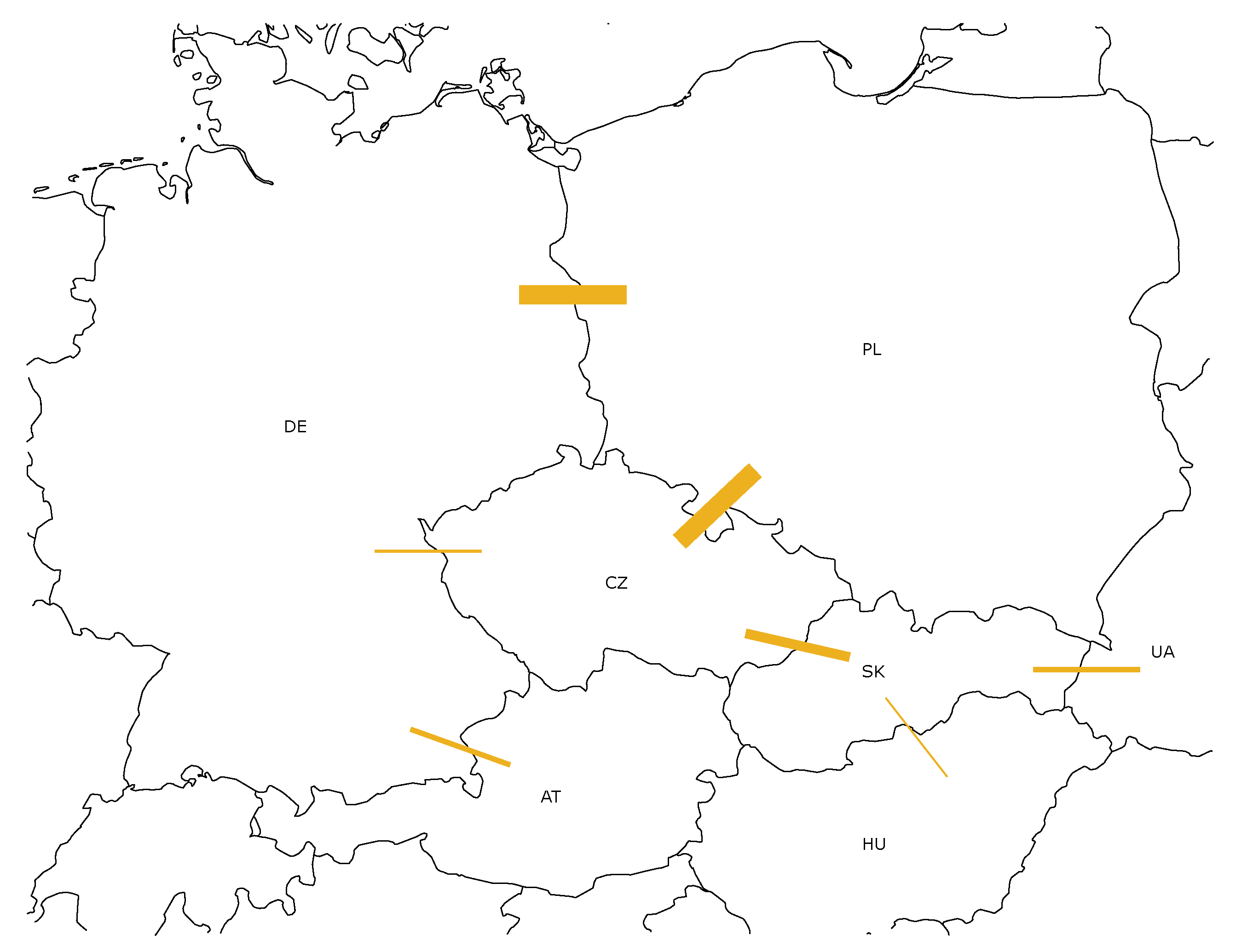
• Candidate CBCOs were identified with COs selected out of the XB connections and their nearest neighbors—intra-zonal lines terminating at the border stations.
• The LODFs for all candidate CBCO pairs were calculated.
• The final CBCOs were identified as the ones for which the absolute value LODF was greater than the threshold selected as 5%.

That method resulted in the CBCO set having around 1200 CBCOs to be included in the congestion management model. In order to model the power flows in the optimization model, two competing approaches were used, both equivalent to a DC Power Flow approximation. The first approach is based on the standard DC Power Flow formulation [21], which was modified to allow varying the branch phase shift angle with respect to tap shifting for branches containing a PST. The second formulation is based on Power Transfer Distribution Factors (PTDFs) and Phase Shifter Distribution Factors (PSDFs) [22,23]. Both formulations are given below. The modified DC Power Flow formulation proved to be computationally more efficient in solving the congestion management optimization problem—around 20 times faster than the formulation based on PTDFs and PSDFs (with the Gurobi 8 optimizer used in both cases), with also better scaling when increasing the number of CBCOs in the model. On the other hand, the second formulation served to obtain the Lagrange multipliers for one of the methods of selecting the candidate locations of new PSTs. The general optimization problem is formulated with the following objective function (OF), representing the congestion management costs:

$$\underset{\mathbf{V}}{min}\sum _{i=1}^{N_T}\left(T_i^{+}{C}_{T_i}^{+}-T_i^{-}{B}_{T_i}^{-}\right)+\sum _{i=1}^{N_R}{R}_i^{-}{C}_{\mathrm{curt}}+\sum _{i=1}^{N_E}{E}_i^{+}{C}_{\mathrm{VOLL}},$$

(1)

which is to be minimized with respect to the vector variables (for the sake of conciseness, we use bold font to denote vector variables, that is, $\mathbf{X}=(X_1,X_2,X_3,\dots )$):

$$\mathbf{V}=\{{\mathbf{T}}^{+}-{\mathbf{T}}^{-},{\mathbf{R}}^{-},{\mathbf{E}}^{+},\mathbf{S}\},$$

(2)

where:

• $T_i^{+}$ is the power shift up of thermal generator i;
• $T_i^{-}$ is the power shift down of thermal generator i;
• $R_i^{-}$ is the curtailed power of RES generator i;
• $E_i^{+}$ is the variable representing the energy curtailment of the demand or Energy Not Served per demand in bus i;
• $S_i$ is the variable representing the tap setting of PST i.

Additionally:

• $N_T$ is the number of thermal generators in the system;
• $N_E$ is the number of loads in the system;
• $N_R$ is the number of RES generators in the system;
• $C_{T_i}^{+}$ is the cost of regulating up thermal generator i;
• $B_{T_i}^{-}$ is the revenue from regulating down thermal generator i;
• $C_{\mathrm{curt}}$ is the penalty cost for curtailment of RES;
• $C_{\mathrm{VOLL}}$ is the penalty cost for the energy curtailment.

Finally, the constraints are defined as follows:

$$\begin{array}{cc}\hfill & {\forall }_{\mathrm{CBCO}\in \mathbf{CBCO}} |F_{\mathrm{CBCO}}^0+\Delta F_{\mathrm{CBCO}}\left(\mathbf{V}\right)|\le F_{\mathrm{CBCO}}^{max},\hfill \end{array}$$

(3)

$$\begin{array}{cc}\hfill & {\forall }_{i\in \{1,\dots ,N_T\}} T_i^{+}\in \left[0,T_i^{max}-T_i^0\right],\hfill \end{array}$$

(4)

$$\begin{array}{cc}\hfill & {\forall }_{i\in \{1,\dots ,N_T\}} T_i^{-}\in \left[0,T_i^0-T_i^{min}\right],\hfill \end{array}$$

(5)

$$\begin{array}{cc}\hfill & {\forall }_{i\in \{1,\dots ,N_R\}} R_i^{-}\in \left[0,R_i^0\right],\hfill \end{array}$$

(6)

$$\begin{array}{cc}\hfill & {\forall }_{i\in \{1,\dots ,N_S\}} S_i\in \left[S_i^{min}-S_i^0,\dots ,S_i^{max}-S_i^0\right],\hfill \end{array}$$

(7)

$$\begin{array}{cc}\hfill & \mathrm{Balance}\left(\mathbf{V}\right)=0,\hfill \end{array}$$

(8)

where:

• $F_{\mathrm{CBCO}}^{max}$ is the power capacity limit for transmission line CB;
• $F_{\mathrm{CBCO}}^0$ is the initial power flow over line CB in outage state of CO;
• $T_i^0$ is the initial generation point in power of thermal generator i;
• $T_i^{max}$, $T_i^{min}$ are, respectively, the maximal and minimal operating power limit of thermal generator i;
• $R_i^0$ is the initial generation point in power of RES generator i;
• $N_S$ is the number of PSTs in the system;
• $S_i^0$ is the initial tap setting of PST i;
• $S_i^{max}$, $S_i^{min}$ are, respectively, the maximal and minimal tap setting of PST i;
• $\mathrm{Balance}\left(\mathbf{V}\right)=0$ is a set of nodal balance equations;
• $\Delta F_{\mathrm{CBCO}}\left(\mathbf{V}\right)$ is the set of the flow equations.

The formulations of the two last constraints depend on the chosen approach to power flow modeling, as described in the following two subsections.

3.2. Modified DC Power Flow Formulation

For the modified DC Power Flow formulation, the

$$\mathrm{Balance}\left(\mathbf{V}\right)\equiv \mathrm{Balance}(T^{+}-T^{-},R^{-},E^{+},S)=0$$

condition is represented by a set of nodal power balance equations, which depend on the power injections of thermal generating units, RES and Energy Not Served (ENS) volumes, as well as the tap settings of PSTs:

$${\forall }_{j\in \{1,\dots ,N_B\}} {\mathrm{NodalBalance}}_j\left(\mathbf{V}\right)=0,$$

(9)

where $N_B$ is the number of buses in the grid model, while the $\Delta F_{\mathrm{CBCO}}\left(\mathbf{V}\right)$ (cf. (3)) represents the change in CBCO flow due to shifts in generation/PST taps. Both ${\mathrm{NodalBalance}}_j\left(\mathbf{V}\right)$ and $\Delta F_{\mathrm{CBCO}}\left(\mathbf{V}\right)$ are implicitly modelled as a set of DC Power Flow equations depending on the nodal active power injections, which in turn depend on bus voltage angles.

3.3. PSDF and PTDF Formulation

For the PSDF and PTDF formulation, the $\mathrm{Balance}\left(\mathbf{V}\right)=0$ condition is represented by a single equation representing the redispatch/RES curtailment balance:

$$\sum _{i=1}^{N_T}(T_i^{+}-T_i^{-})-\sum _{i=1}^{N_R}{R}_i^{-}+\sum _{i=1}^{N_E}{E}_i^{+}=0,$$

(10)

while the following:

$$\begin{array}{cc}\hfill \Delta F_{\mathrm{CBCO}}\left(\mathbf{V}\right)& =\sum _{i=1}^{N_T}{\mathrm{PTDF}}_{\mathrm{CBCO}}^{T_i}·(T_i^{+}-T_i^{-})+\hfill \\ \hfill & -\sum _{i=1}^{N_R}{\mathrm{PTDF}}_{\mathrm{CBCO}}^{R_i}·R_i^{-}+\hfill \\ \hfill & +\sum _{i=1}^{N_E}{\mathrm{PTDF}}_{\mathrm{CBCO}}^{E_i}·E_i^{-}+\hfill \\ \hfill & +\sum _{i=1}^{N_S}{\mathrm{PSDF}}_{\mathrm{CBCO}}^{S_i}·A_{S_i}·S_i\hfill \end{array}$$

(11)

constitutes the flow equation for a CBCO, where: ${\mathrm{PTDF}}_{\mathrm{CBCO}}^{T_i}$, ${\mathrm{PTDF}}_{\mathrm{CBCO}}^{R_i}$, ${\mathrm{PTDF}}_{\mathrm{CBCO}}^{E_i}$ are, respectively, the PTDF coefficients for a change of flow over the CBCO with respect to bus of generator $T_i$, RES generator $R_i$, and ENS bus $E_i$; ${\mathrm{PSDF}}_{\mathrm{CBCO}}^{S_i}$ is the PSDF coefficient of flow over the CBCO with respect to phase angle of PST $S_i$, and $A_{S_i}$ is the change of angle of PST $S_i$ per one tap setting. For CBCO pairs, the the appropriate PTDF values were derived using Line Outage Distribution Factors (LODF) in the following way:

$${\mathrm{PTDF}}_{\mathrm{CBCO}}^{T_i}={\mathrm{PTDF}}_{\mathrm{CB}}^{T_i}+{\mathrm{LODF}}_{\mathrm{CBCO}}·{\mathrm{PTDF}}_{\mathrm{CO}}^{T_i},$$

where ${\mathrm{PTDF}}_{\mathrm{CB}}^{T_i}$ and ${\mathrm{PTDF}}_{\mathrm{CO}}^{T_i}$ are the PTDFs with respect to the bus of generator $T_i$ for CB and CO, respectively; the PSDF coefficients for CBCO pairs are derived in the same manner.

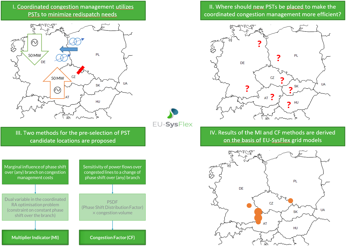
4. Theoretical Description—Methods for Pre-Selecting the Candidates of the PST Investments

This section will introduce the two methods we propose for the purpose of the pre-selection of PST candidate locations. Both methods aim at identifying the locations with the highest potential to decrease the cost of remedial actions applied by the congestion management model.

4.1. Multiplier Indicator (MI)

The first method is based on Lagrange multipliers—the values assigned to constraints defined in the optimization problem, which carry the information about the effect that a marginal variation of the right-hand side of a particular constraint has on the value of the objective function in the optimal point.

For the purpose of obtaining the multiplier indicators, the congestion management model in the PSDF and PTDF formulation was built (see Section 3.3) for each grid scenario, in which:

• A possibility of changing the phase angle of each branch in the model was added—each branch is allowed to introduce a phase shift $L_i$ like a PST. In particular, the new power flow equations now take the following form:

  $$\begin{array}{cc}\hfill {\overline{\Delta F}}_{\mathrm{CBCO}}\left({\mathbf{V}}_{\mathbf{L}}\right)& =\Delta F_{\mathrm{CBCO}}\left({\mathbf{V}}^{🟉}\right)+\hfill \\ \hfill & +\sum _{i=1}^{N_L}{\mathrm{PSDF}}_{\mathrm{CBCO}}^{L_i}·A_{L_i}·L_i,\hfill \end{array}$$

  (12)

  where:
  • ${\mathrm{PSDF}}_{\mathrm{CBCO}}^{L_i}$ is the PSDF coefficient of flow over CBCO with respect to phase angle $L_i$ of branch i (acting like a PST),
  • $A_{L_i}$ is the angle per tap sensitivity assigned to branch i—the change of the phase angle resulting from shifting one tap (a reference value of $A_{L_i}$, based on the values for existing PSTs, is used for the “candidates”)
  • $N_L$ is the number of branches in the grid,
  • $S_i^{🟉}$ are the optimal tap settings of existing PSTs, obtained in the cross-border congestion management optimal solution for the given grid scenario,
  • ${\mathbf{V}}^{🟉}=\{{\mathbf{T}}^{+}-{\mathbf{T}}^{-},{\mathbf{R}}^{-},{\mathbf{E}}^{+},{\mathbf{S}}^{🟉}\}$ is the set of vector variables from Equation (2) with the optimal PST tap settings,
  • ${\mathbf{V}}_{\mathbf{L}}=\{{\mathbf{T}}^{+}-{\mathbf{T}}^{-},{\mathbf{R}}^{-},{\mathbf{E}}^{+},\mathbf{L}\}$ is the modified set of vector variables.
• The new phase shift $L_i$ is set to a parameter ${\alpha }_i$, by additional constraints:

  $${\forall }_{i\in \{1,\dots ,N_L\}} L_i={\alpha }_i.$$

  (13)

  When solving the optimization model, the extra constraints defined above with parameters ${\alpha }_i$ all set to zero allow deriving the Lagrange multipliers associated with keeping the phase shift of each branch constant. Then, the multiplier for branch i can be interpreted as the cost-benefit from a marginal phase shift of candidate PST assigned to that branch.
• The $\mathbf{L}$ variables are defined as continuous, which makes the optimization problem continuous (not MILP) and thus the Lagrange multipliers of each constraint can be obtained.

The mathematical description of the procedure of obtaining the multiplier indicators—namely, estimators of the sensitivities of the congestion management cost (the objective function) to the marginal phase shift of each PST candidate—is given below. The starting point is the Lagrangian of the problem defined above, limited to the elements that depend on the ${\alpha }_i$ parameters:

$$\begin{array}{cc}\hfill \mathcal{L}& =\mathrm{OF}\left(\mathbf{V}\right)+\hfill \\ \hfill & +\sum _{\mathrm{CBCO}\in \mathbf{CBCO}}{\mu }_{\mathrm{CBCO}}^{+}\left({\overline{\Delta F}}_{\mathrm{CBCO}}\left({\mathbf{V}}_{\mathbf{L}}\right)-F_{\mathrm{CBCO}}^{max}+F_{\mathrm{CBCO}}^0\right)+\hfill \\ \hfill & +\sum _{\mathrm{CBCO}\in \mathbf{CBCO}}{\mu }_{\mathrm{CBCO}}^{-}\left({\overline{\Delta F}}_{\mathrm{CBCO}}\left({\mathbf{V}}_{\mathbf{L}}\right)-F_{\mathrm{CBCO}}^{max}-F_{\mathrm{CBCO}}^0\right)+\hfill \\ \hfill & +\sum _{i=1}^{N_L}{\lambda }_i·(L_i-{\alpha }_i),\hfill \end{array}$$

(14)

where the following Lagrange multipliers were introduced:

• ${\mu }_{\mathrm{CBCO}}^{+}$ and ${\mu }_{\mathrm{CBCO}}^{-}$—assigned to constraints limiting power flows for CBCOs (in both directions),
• ${\lambda }_i$—assigned to constraints setting the phase angles equal to ${\alpha }_i$.

Applying the envelope theorem with respect to the ${\alpha }_i$ parameter allows us to obtain the value function in the form:

$$\begin{array}{cc}\hfill \mathrm{VF}\left({\alpha }_i\right)& \equiv \mathrm{OF}\left({\mathbf{V}}^{🟉}\left({\alpha }_i\right)\right),\hfill \\ \hfill {\mathbf{V}}^{🟉}\left({\alpha }_i\right)& =\left\{{\mathbf{T}}^{+🟉}\left({\alpha }_i\right)-{\mathbf{T}}^{-🟉}\left({\alpha }_i\right),{\mathbf{R}}^{-🟉}\left({\alpha }_i\right),{\mathbf{E}}^{+🟉}\left({\alpha }_i\right),{\mathbf{L}}^{🟉}\left({\alpha }_i\right)\right\},\hfill \end{array}$$

(15)

where the star superscripts are used to describe the optimal values of control variables, that satisfies the following equations:

$${\forall }_{i\in \{1,\dots ,N_L\}} {\displaystyle \frac{\partial \mathrm{VF}\left({\alpha }_i\right)}{\partial {\alpha }_i}}={\displaystyle \frac{\partial {\mathcal{L}}^{🟉}\left({\alpha }_i\right)}{\partial {\alpha }_i}}=-{\lambda }_i,$$

(16)

allowing the calculation of the multipliers ${\lambda }_i$, with ${\mathcal{L}}^{🟉}$ being the Lagrangian in the optimal solution. As the sign of the multiplier is of a less importance (the congestion management cost might be decreased either by lowering or increasing the phase shift on a given branch), the absolute value of the multiplier, $|{\lambda }_i|$, should be defined as the “multiplier indicator” for placing a PST in the location of branch i for the analyzed grid scenario (scen) as it indicates how that candidate could influence the congestion management cost in the optimal point, namely:

$${\mathrm{MI}}_{L_i}^{\mathrm{scen}}=\left|{\lambda }_i\right|.$$

(17)

The method of calculating the multiplier indicators, when used for a set of representative hourly system scenarios (the set $\mathbf{scen}$), may provide insights relevant from the perspective of long-term investment planning. In particular, multipliers collected for a given branch may be aggregated, e.g., by calculating their sum, direct or weighted by probabilities assigned to analyzed system scenarios. Such a value could be considered as the “total absolute multiplier indicator” and be used to rank the branches to select the ones providing the locations where the investment in a new PST would be more profitable:

$${\mathrm{MI}}_{L_i}\sum _{\mathrm{scen}\in \mathbf{scen}}={\mathrm{MI}}_{L_i}^{\mathrm{scen}}.$$

(18)

Afterwards, a selected number of candidates with the highest rank with respect to ${\mathrm{MI}}_{L_i}$ value could be the object of further examination, e.g., expert-based analysis by the TSO or cost-benefit analysis by the decision makers.

4.2. Congestion Factor (CF)

In this subsection, we depict the method of identifying the locations, where a PST would be most effective in relieving congestions. It is based on ranking the locations (branches) by the congestion factor (CF), which for branch $L_i$ and scenario $\mathrm{scen}$ is defined as:

$${\mathrm{CF}}_{L_i}^{\mathrm{scen}}=|\sum _{\mathrm{CBCO}\in \mathbf{CBCO}}{\mathrm{CV}}_{\mathrm{CBCO}}^{\mathrm{scen}}·{\mathrm{TSDF}}_{\mathrm{CBCO}}^{L_i}|,$$

(19)

where:

• ${\mathrm{TSDF}}_{\mathrm{CBCO}}^{L_i}={\mathrm{PSDF}}_{\mathrm{CBCO}}^{L_i}·A_{L_i}$ is the so-called Tap-Shift Distribution Factor (TSDF) joining the PSDF and the angle per tap sensitivity of the branch i,
• ${\mathrm{CV}}_{\mathrm{CBCO}}^{\mathrm{scen}}$ is the congestion volume for a CBCO in grid scenario $\mathrm{scen}$, which is the value of power flow over the CB line that exceeds its thermal limit, defined by Equation (20) with:

  –

  ${\mathbf{V}}_{\mathbf{0}}^{🟉}=\{\mathbf{0},\mathbf{0},\mathbf{0},{\mathbf{S}}^{🟉}\}$—the set of vector variables in the optimal point including zero-valued vectors,

  –

  ${\mathbf{S}}^{🟉}$—the vector of optimal tap settings of the existing PSTs for the scenario $\mathrm{scen}$.

$$\begin{array}{cc}\hfill & {\mathrm{CV}}_{\mathrm{CBCO}}^{\mathrm{scen}}=\hfill \\ \hfill & =\left\{\begin{array}{cc}\Delta F_{\mathrm{CBCO}}\left({\mathbf{V}}_{\mathbf{0}}^{🟉}\right)-F_{\mathrm{CBCO}}^{\max }, \hfill & \mathrm{if} F_{\mathrm{CBCO}}\left({\mathbf{V}}_{\mathbf{0}}^{🟉}\right)\ge F_{\mathrm{CBCO}}^{\max },\hfill \\ \Delta F_{\mathrm{CBCO}}\left({\mathbf{V}}_{\mathbf{0}}^{🟉}\right)+F_{\mathrm{CBCO}}^{\max }, \hfill & \mathrm{if} F_{\mathrm{CBCO}}\left({\mathbf{V}}_{\mathbf{0}}^{🟉}\right)<F_{\mathrm{CBCO}}^{\max }.\hfill \end{array}\right.\hfill \end{array}$$

(20)

Most importantly, the congestion volumes ${\mathrm{CV}}_{\mathrm{CBCO}}^{\mathrm{scen}}$ are obtained in the state resulting from the congestion management model run exactly as described in Section 3, however with the remedial actions that are taken into account from the optimal solution limited only to PSTs settings (no redispatch or RES curtailment generation shifts are taken into account when calculating the ${\mathrm{CV}}_{\mathrm{CBCO}}^{\mathrm{scen}}$ volumes). It means that non-zero values of congestions volumes, if found, are the ones that the existing PSTs were not capable of relieving despite being at optimal tap settings. Additionally, by taking into account the direction of the congestion, the ${\mathrm{CV}}_{\mathrm{CBCO}}^{\mathrm{scen}}$ measure is sensitive to potential conflict in phase shift direction the relief of the set of congested lines calls for. Hence, the congestion factor is created as an indicator of potentials that PST candidates (considered in locations of all branches in the grid) have on relieving the remaining congestion volume. That idea is reflected in the CF definition for each PST candidate by juxtaposing its TSDFs—sensitivities with respect to congested CBCOs—with the volume of those congestions. For the long-term investment planning point of view, we could extract this congestion factor per each hourly simulation or representative system scenario (the set $\mathbf{scen}$), and aggregate them by the sum of them or the weighted sum depending on the probability of the representative scenario. From now on, we refer by CF to the aggregation of the indicator over the scenarios of the study:

$${\mathrm{CF}}_{L_i}=\sum _{\mathrm{scen}\in \mathbf{scen}}{\mathrm{CF}}_{L_i}^{\mathrm{scen}}.$$

(21)

The CF, defined using the congestion volume, allows us to identify which PST investment has the highest impact on the overloaded lines. The main limitation of CFs is that their impact on the non-overloaded CBCOs is ignored. Hence, the PST investment selected according to the highest CF might not be the most profitable—it may relieve the congested CBCOs but cause the congestions of some other.

4.3. Combined Methodology for Pre-Selecting the PST Candidates

This section discusses how to combine both indicators, namely the multiplier indicator (MI introduced in Section 4.1) and the congestion factor (CF introduced in Section 4.2), for the PST candidates pre-selection. The CF provides information about the potential the PST candidates have for relieving congestions. Nonetheless, the information of how a PST candidate would affect other non-congested lines is not provided by the CF. This means that the benefits found for the particular PST candidate as resulting from removing congestions might be overestimated, due to not including the overloads caused by the actions of that PST candidate. On the other hand, the multiplier indicator provides an estimation of how economically profitable a given PST candidate is. Hence, a hierarchical approach could be considered, with MI used to identify only the profitable PST candidates. Afterwards, the CF might be applied to make the final choice based on the potential of relieving congestions. Therefore, the proposed approach would utilize the advantages of both indicators. However, it would also suffer from the limitation both methods have, namely being valid for the initial analysis of PSTs located only next to existing branches.

5. EU-SysFlex Scenarios

As the input data used for obtaining the results presented in the article, we used a set of 24 scenarios developed as a part of the H2020 EU-Sysflex project [24,25,26], which cover a significant part of the Continental European synchronous power system in specific conditions, namely minimal inertia, maximal demand and minimal reactive power availability in selected countries. The power system models used within the scenarios contained the following national grids:

• with high detailed resolution: Poland, Germany, Czech Republic, Slovakia,
• with medium detailed resolution: Austria, Hungary, Ukraine,
• an equivalent representation of other European countries connected to the synchronous grid.

The scenarios consist of around 15,000 buses, 17,000 lines and 1200 generators. Across the grid, 15 phase shifting transformers in five locations were identified. The grid models representing those scenarios were converted to the MPC case format to be analyzed in the Matlab environment with the Matpower [27] package.

6. Results

In this section we present the results of the congestion management model and of the two methods for pre-selecting PST candidates, as derived from the EU-Sysflex scenarios.

6.1. Congestion Management Model

First, we show and discuss the results of the application of the congestion management model to the EU-SysFlex scenarios (described in Section 5). The congestion management model was run on the 24 grid scenarios to identify the congestions and obtain the cost-effective tap settings of the PSTs and redispatch/RES curtailment volumes that relieve them. Across 24 grid scenarios, in 21 of them congestions were identified among at least one line from the $\mathbf{CBCO}$ set—Figure 1 depicts their locations and severity.

Table 1. Average congestion severity (when the congestion is non-zero) and total number of congested CBCOs per border across 24 grid scenarios. Source: own calculations.

Border	Average Congestion [MW]	Number of Congestions
DE-AT	35.61	25
PL-CZ	129.16	26
CZ-SK	48.48	35
SK-UA	75.26	12
PL-DE	140.06	24
DE-CZ	99.14	5
SK-HU	42.71	6

shows the extent of identified congestions per cross border profile and reveals the fact that most frequent congestions appear on the Czech–Slovak border, however, their severity is relatively low. The most severe congestions appear on Polish–Czech and Polish–German interconnections. In 14 out of 24 grid scenarios, the congestion management model cleared the congestions using only PSTs, which is in costless fashion. Moreover, no ENS nor RES curtailment was needed to clear the congestions in any of the scenarios.

In order to illustrate the economic impact the PSTs have on the congestion management, the model was run again in a such a manner that the PSTs were kept on their initial tap settings.

Table 2. Comparison of congestion management costs aggregated over 24 grid scenarios, maximal congestion management costs across 24 grid scenarios, and total redispatch volumes across 24 grid scenarios with and without the use of phase-shifting transformers (PSTs). Source: own calculations.

PST Usage	Total Congestion Management Cost [EUR]	Maximal Congestion Management Cost [EUR]	Total Volume of Redispatching [MW]
Used	12,579.28	2561.32	3573.09
Not used	134,023.58	58,598.78	16,435.82

shows the comparison of costs of relieving the congestions in both cases—with and without using PSTs. It reveals the fact that the congestion management costs rose tenfold when no PSTs were used to relieve the congestions, with the volume of required redispatching rising over four times.

Having obtained the congestion management costs for the existing PSTs, in the next two subsections we present the results of the methods for pre-selecting the new PST candidate locations. In this context, the previous use cases are considered as representative scenarios of the year, which allowed using the aforementioned methods to evaluate the annual impact of the top candidates on the power system.

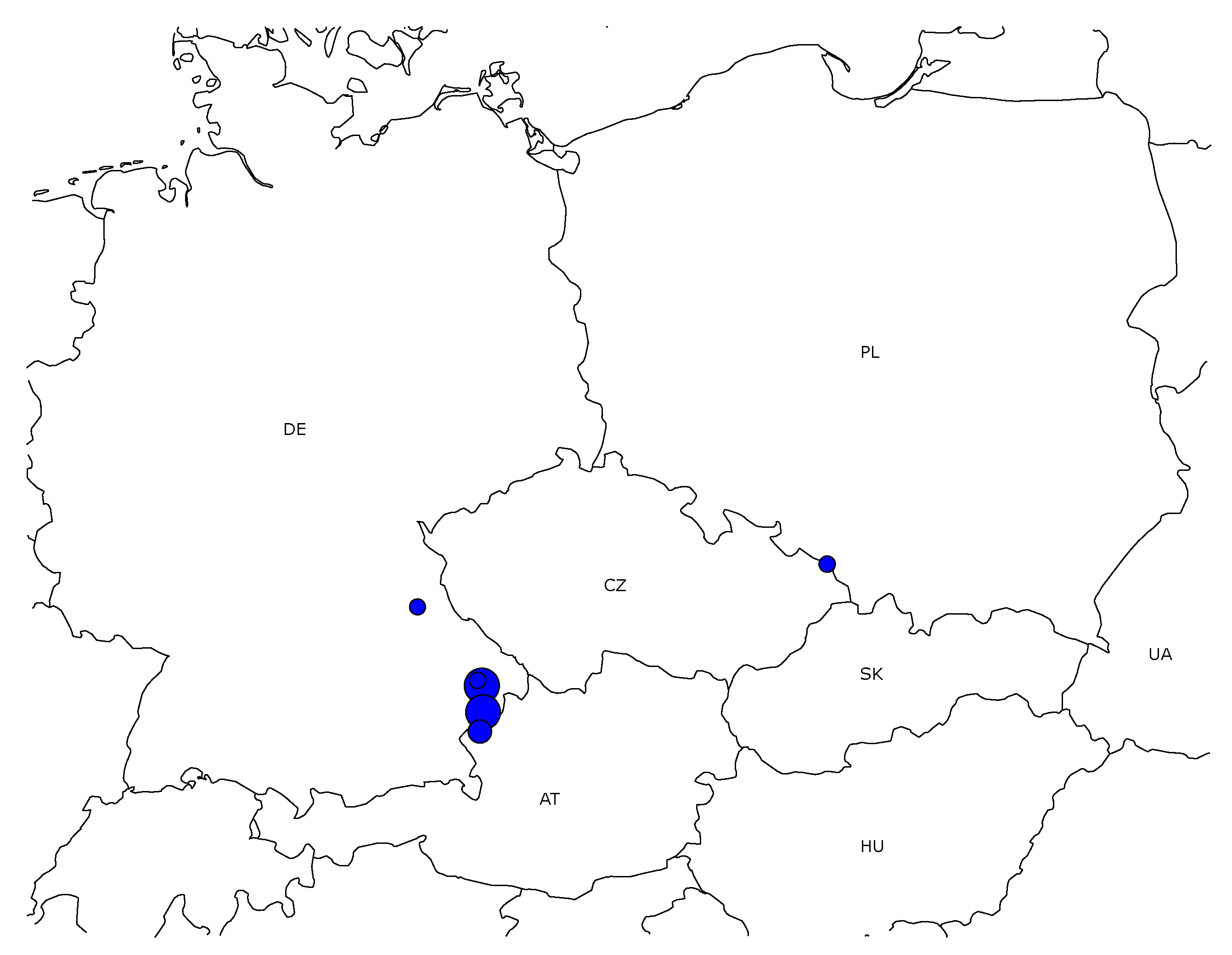
6.2. Long-Term Analysis—Candidate Selection for PST Investments

As a starting point for obtaining the relevant indicators, we use grid states in which the existing PSTs are set on their optimal tap settings derived from the congestion management model, but no redispatching is yet done in the system.

6.2.1. Multiplier Indicator Method

An optimization model defined in Section 4.1 was used to obtain the MI values for all the branches of the system across 24 grid scenarios, with the resulting top 9 MI values given in

Table 3. Top 9 (cut-off at multiplier indicator (MI) = 600) branches according to the multiplier indicators and congestion management costs, aggregated over 24 grid scenarios, obtained after placing a new PST at a given branch. (The letters A–I in parentheses serve as identifiers of locations to be compared with congestion factor (CF) results in Table 4 below). Source: own calculations.

Branch Location	MI	Congestion Management Costs [EUR]
line (A) on DE-AT border	3045.15	394
DE station (B) next to DE-AT border	1285.90	808
DE transformer (C) next to DE-AT border	916.84	490
DE transformer (D) next to DE-AT border	866.77	641
line (E) on DE-AT border	695.62	5391
line (F) on DE-AT border	690.63	5422
DE line (G) next to DE-AT border	651.30	2007
line (H) on PL-CZ border	629.70	9407
DE line (I) next to DE-AT border	610.58	2335

below. Then, in order to validate the pre-selection suggested by the proposed indicators, the congestion management model was run again with a new PST in operation, for each of the nine locations independently and all 24 grid scenarios. The congestion management costs obtained in such a way are also presented in Table 3, while the map in Figure 2 displays the top 9 MI values aggregated into six locations (the aggregation joins the branches in one geographical location, for example transformers (C) and (D) and branch in station (B) from Table 3).

The multiplier indicators (cf. Table 3) point out that a new PST should be located in German station next to German–Austrian cross-border connection, where most of the MI “weight” of the indicators are concentrated. The congestion management costs (cf. Table 3) decrease after a new PST is placed in locations in that station or in its neighborhood confirm that choice of investment. A second PST candidate location which is significantly further away from the German–Austrian border station, the Polish–Czech branch, has significantly lower MI values, as well as a lower decrease in congestion management costs estimation.

Comparing the MI values in Figure 2 with the congestion volumes shown in Table 1 and Figure 1, we note that the Polish–German and Polish–Czech borders, on which the congestions volume-wise are the most severe, do not appear as the top locations according to MI values. Apparently, those congestions are relatively easily addressed using the existing PSTs, while the congestions near German–Austrian border are the hardest (or most costly) to clear in the current topology.

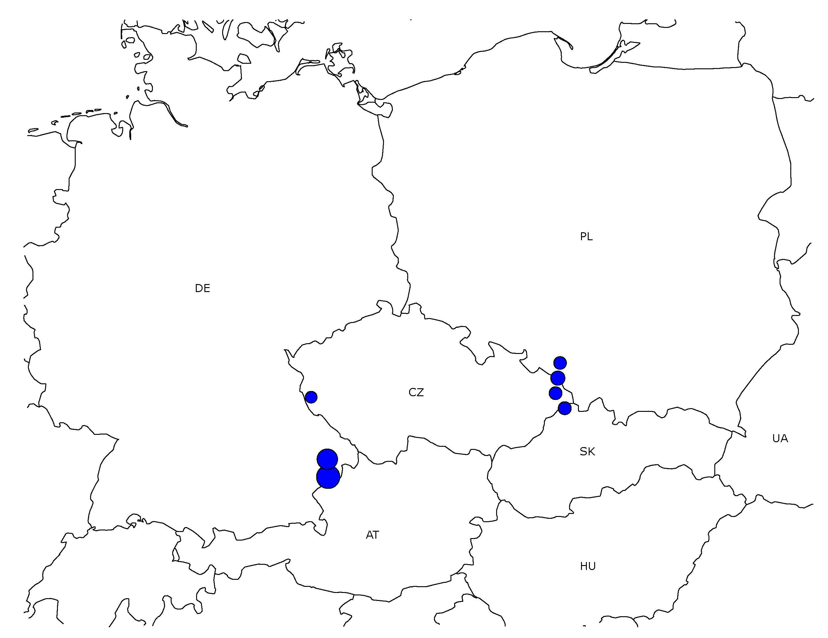
6.2.2. Congestion Factor Method

To obtain the CF values, we estimated the CBCOs overload volumes in the grid scenario modified by setting the existing PSTs at the optimal values derived from the congestion management model solution. The CF results for the top 8 locations, aggregated across 24 grid scenarios, are given in

Table 4. Top 8 (cut-off at CF = 5000) branches according to the congestion factors and congestion management costs, aggregated over 24 grid scenarios, obtained after placing a new PST at a given branch. (The letters in parentheses serve as identifiers of locations to be compared with MI results in Table 3 above). Source: own calculations.

Branch Location	CF	Congestion Management Costs [EUR]
line (A) on DE-AT border	21,441.05	394
DE station (B) next to DE-AT border	11,078.74	808
line (H) on PL-CZ border	7436.30	9407
line (J) on CZ-SK border	6343.77	9569
CZ station (K) next to PL-CZ border	6142.07	10,474
PL station (L) next to PL-CZ border	5908.53	9454
DE transformer (C) next to DE-AT border	5319.99	490
line (M) on DE-CZ border	5163.14	3546

.

As for the MI approach, for each of the eight locations, a PST was added there, and congestion management costs were evaluated for validation of this new PST in operation using the congestion management model. The congestion management costs are also displayed in Table 4. The map in Figure 3 displays the top 8 CF values aggregated into 7 locations.

The calculated congestion factors (cf. Table 4) are again the highest for a location on the German side of the German–Austrian cross-border line, although the results are less unanimous than those based on MIs, with candidate location more spread geographically among the top values of CF. However, the estimated decrease in the congestion management costs after placing a PST in the candidate location (cf. Table 4) again points to the German side of the German–Austrian cross-border line as the most promising candidate. As it was the case with MI approach, also here we note that the most severe congestions on the Polish–German and Polish–Czech borders (cf. Figure 1) do not result in the highest congestion factors: again, these are the congestions near the German–Austrian border which, although being of relatively low volume, are the hardest to manage using existing PSTs.

6.2.3. Summary of the Validation Results

We note that both methods ranked the same element/location as the best candidate. After placing the new PST there (a German station next to DE-AT border), the congestions could be relieved using only costless PST tap switching in 22 out of 24 scenarios. For the remaining 2 scenarios, the total congestion management cost amounted to 394 EUR, which is less than 1/30 of the total congestion management cost for the existing PSTs reported in Table 2 (and the lowest cost achieved for any of the discussed candidates). The lower positions of the rankings, both MI-based and CF-based, do not perfectly match the ordering of congestion management costs derived in the validation phase. That is why further study of the investment candidates by a CBA or another, more detailed optimization stage, is needed. Nonetheless, the PST pre-selection methods described in the paper seem to be promising in identifying the best candidates from the perspective of cost efficiency of coordinated congestion management.

7. Conclusions

The first aim of this paper was to prove that the European Union policy of coordinating the congestion management process among European TSOs is feasible for large-scale systems (with over 10,000 branches or nodes, cf. Section 5). Furthermore, motivated by the computational challenges of the PSTs optimal siting methods, we proposed two approaches to pre-selecting candidate sites for new PSTs, both derived from the optimization problem used in the coordinated cross-border congestion management model, that we developed within the H2020 EU-SysFlex project. Both methods were described in this paper as providing indicators for the pre-selection of sites for new PSTs. The first indicator, referred to as MI (Section 4.1), provides the economic profitability of the candidate PST location, while the second, CF (Section 4.2), is able to estimate the potential the PST candidate location has for relieving congestions. The results for both indicators have been obtained for the European power system models prepared for the EU-SysFlex project and described in this paper. The discussion of the advantages, disadvantages and possibilities for extension of the introduced methods is also included, along with an important conclusion that coupling both methods for the purpose of obtaining a more comprehensive PST candidate pre-selection is possible (Section 4.3).

References

1. Regulation (EU) 2019/943 of the European Parliament and of the Council of 5 June 2019 on the internal market for electricity. Offic J. Eur. Union 2019, L 158, 54–124.
2. Commission Regulation (EU) 2017/1485 of 2 August 2017 establishing a guideline on electricity transmission system operation. Offic. J. Eur. Union 2017, L 220, 1–120.
3. Commission Regulation (EU) 2015/1222 of 24 July 2015 establishing a guideline on capacity allocation and congestion management. Offic. J. Eur. Union 2015, L 197, 24–72.
4. Korab, R.; Owczarek, R. Impact of phase shifting transformers on cross-border power flows in the Central and Eastern Europe region. Bull. Pol. Acad. Sci. Tech. Sci. 2016, 64, 127–133. [Google Scholar] [CrossRef]
5. Korab, R.; Owczarek, R.; Połomski, M. Coordinated Control of Phase Shifting Transformers in the Power System. Acta Energetica 2017, 3/32, 97–103. [Google Scholar]
6. Commission for Electricity and Gas Regulation. Study on the Best Forecast of Remedial Actions to Mitigate Market Distortion; CREG Study (F)1987. Commission for Electricity and Gas Regulation: Bruxelles, Belgium, 2019. Available online: https://www.creg.be/sites/default/files/assets/Publications/Studies/F1987EN.pdf (accessed on 20 July 2020).
7. Verboomen, J.; Van Hertem, D.; Schavemaker, P.H.; Kling, W.L.; Belmans, R. Analytical approach to grid operation with phase shifting transformers. IEEE Trans. Power Syst. 2008, 23, 41–46. [Google Scholar] [CrossRef]
8. Jordehi, A.R. Optimal allocation of FACTS devices for static security enhancement in power systems via imperialistic competitive algorithm (ICA). Appl. Soft Comput. 2016, 48, 317–328. [Google Scholar] [CrossRef]
9. Miranda, V.; Alves, R. PAR/PST location and sizing in power grids with wind power uncertainty. In Proceedings of the 2014 International Conference on Probabilistic Methods Applied to Power Systems (PMAPS), Durham, NC, USA, 7–10 July 2014; pp. 1–6. [Google Scholar]
10. Bekaert, D.; Meeus, L.; Van Hertem, D.; Delarue, E.; Delvaux, B.; Kupper, G.; Belmans, R.; D’Haeseleer, W.; Deketelaere, K.; Proost, S. How to increase cross border transmission capacity? A case study: Belgium. In Proceedings of the 2009 6th International Conference on the European Energy Market, Leuven, Belgium, 27–29 May 2009; pp. 1–6. [Google Scholar]
11. Ippolito, L.; Siano, P. Selection of optimal number and location of thyristor-controlled phase shifters using genetic based algorithms. IEEE Proc. Gener. Transm. Distrib. 2004, 151, 630–637. [Google Scholar] [CrossRef]
12. Hadzimuratovic, S.; Fickert, L. Determination of critical factors for optimal positioning of Phase-Shift Transformers in interconnected systems. In Proceedings of the 2018 19th International Scientific Conference on Electric Power Engineering (EPE), Brno, Czech Republic, 16–18 May 2018; pp. 1–6. [Google Scholar]
13. Paterni, P.; Vitet, S.; Bena, M.; Yokoyama, A. Optimal location of phase shifters in the French network by genetic algorithm. IEEE Trans. Power Syst. 1999, 14, 37–42. [Google Scholar] [CrossRef]
14. Lima, F.G.; Galiana, F.D.; Kockar, I.; Munoz, J. Phase shifter placement in large-scale systems via mixed integer linear programming. IEEE Trans. Power Syst. 2003, 18, 1029–1034. [Google Scholar] [CrossRef]
15. Mekonnen, M.T.; Belmans, R. The influence of phase shifting transformers on the results of flow-based market coupling. In Proceedings of the 2012 9th International Conference on the European Energy Market, Florence, Italy, 10–12 May 2012; pp. 1–7. [Google Scholar]
16. Baczynska, A.; Wierzbowski, M. Market coupling and the impact of cross border flows on the balancing of power demand. In Proceedings of the 2017 14th International Conference on the European Energy Market (EEM), Dresden, Germany, 6–9 June 2017; pp. 1–5. [Google Scholar]
17. Zeraatzade, M.; Kockar, I.; Song, Y.H. Minimizing balancing market congestion re-dispatch costs by optimal placements of FACTS devices. In Proceedings of the 2007 IEEE Lausanne Power Tech, Lausanne, Switzerland, 1–5 July 2007; pp. 873–878. [Google Scholar]
18. Gerbex, S.; Cherkaoui, R.; Germond, A.J. Optimal location of multi-type FACTS devices in a power system by means of genetic algorithms. IEEE Trans. Power Syst. 2001, 16, 537–544. [Google Scholar] [CrossRef]
19. Ahmad, A.A.; Sirjani, R. Optimal placement and sizing of multi-type FACTS devices in power systems using metaheuristic optimisation techniques: An updated review. Ain Shams Eng. J. 2019. [Google Scholar] [CrossRef]
20. Guo, J.; Fu, Y.; Li, Z.; Shahidehpour, M. Direct calculation of line outage distribution factors. IEEE Trans. Power Syst. 2009, 24, 1633–1634. [Google Scholar]
21. Zimmerman, R.; Murillo-Sanchez, C. MATPOWER 5.1 User’s Manual; Power Systems Engineering Research Center (PSERC): Tempe, AZ, USA, 2015; Available online: https://matpower.org/docs/MATPOWERmanual-5.1.pdf (accessed on 20 July 2020).
22. Han, Z.X. Phase Shifter and Power Flow Control. IEEE Trans. Power Appar. Syst. 1982, PAS-101, 3790–3795. [Google Scholar] [CrossRef]
23. Verboomen, J. Optimisation of Transmission Systems by Use of Phase Shifting Transformers. Ph.D. Thesis, TU Delft, Delft, The Netherlands, 2008. [Google Scholar]
24. D2.2. Models for Simulating Technical Scarcities on the European Power System with High Levels of Renewable Generation. Available online: http://eu-sysflex.com/wp-content/uploads/2018/12/D2.2_EU-SysFlex_Scenarios_and_Network_Sensitivities_v1.pdf (accessed on 20 July 2020).
25. D2.3 EU-SysFlex Scenarios and Network Sensitivities. Available online: http://eu-sysflex.com/wp-content/uploads/2018/12/D2.3_Models_for_Simulating_Technical_Scarcities_v1.pdf (accessed on 20 July 2020).
26. D2.4. Technical Shortfalls for Pan European Power System with High Levels of Renewable Generation. Available online: https://eu-sysflex.com/wp-content/uploads/2020/05/EU-SysFlex_D2.4_Scarcity_identification_for_pan_European_-System_V1.0_For-Submission.pdf (accessed on 20 July 2020).
27. Zimmerman, R.D.; Murillo-Sanchez, C.E.; Thomas, R.J. MATPOWER: Steady-state operations, planning and analysis tools for power systems research and education. IEEE Trans. Power Syst. 2011, 26, 12–19. [Google Scholar] [CrossRef] [Green Version]
Figure 1. Congestions on critical branch–critical outages (CBCOs) per borders. The width of the orange line is proportional to the product of average congestion severity (when the congestion is non-zero) and the total number of congested CBCOs per border across 24 grid scenarios. Source: own calculations.
Energies 13 03748 g001
Figure 2. Top 6 locations according to the top 9 MI values (cf. Table 3). The volume of the circle at location is proportional to the MI aggregated for branches in the same location. Source: own calculations.
Energies 13 03748 g002
Figure 3. Top 7 locations according to the top 8 CF values (cf. Table 4). The volume of the circle at location is proportional to the CF aggregated for branches in the same location. Source: own calculations.
Energies 13 03748 g003