Generalized Fixed Point Results with Application to Nonlinear Fractional Differential Equations

Abstract

The main objective of this paper is to introduce the ($\alpha ,\beta$)-type $\vartheta$-contraction, ($\alpha ,\beta$)-type rational $\vartheta$-contraction, and cyclic ($\alpha \text{-}\vartheta$) contraction. Based on these definitions we prove fixed point theorems in the complete metric spaces. These results extend and improve some known results in the literature. As an application of the proved fixed point Theorems, we study the existence of solutions of an integral boundary value problem for scalar nonlinear Caputo fractional differential equations with a fractional order in (1,2).

1. Introduction

Fixed point theorems are useful tools in nonlinear analysis, the theory of differential equations, and many other related areas of mathematics. One of the most applicable method for various investigations is Banach’s contraction principle [1]. Many researchers generalized and extended this theorem to different directions. For example, Boyd and Wong [2] elongated the main result of Banach and they replaced the constant in the contractive condition by an appropriate function. Recently, Samet et al. in [3] defined $\alpha$-admissible and $\alpha$-$\psi$-contractive type mappings and studied some of their properties in the framework of complete metric spaces. Later on, Salimi et al. in [4] introduced and investigated the twisted ($\alpha$,$\beta$)-admissible mappings. Many extensions of the notion of $\alpha$-$\psi$-contractive type mappings have been developed, see, for example, [5,6,7,8,9] and the references therein.

In 2012, Wardowski ([10]) defined $\vartheta$-contraction in the setting of metric space. Wardowski et al. [11] also presented the concept of $\vartheta$-weak contraction and generalized the conception of $\vartheta$-contraction. Kaddouri et al. [12] extended the notion of $\vartheta$-contraction and gave applications of their results to integral inclusions. Arshad et al. in [13] instigated the rational $\vartheta$-contraction and obtained some fixed points results in a metric space. Concerning $\vartheta$-contractions, we mention the researchers in [14,15,16,17,18,19,20,21,22].

In all these investigations, the underlying space was complete metric space. There were some open problems for fixed point theorems in ordered metric spaces and cyclic representations of $\vartheta$-contraction. To solve the first problem, we define ($\alpha$,$\beta )$-type $\vartheta$-contraction with the help of control functions $\alpha$ and $\beta$. With this new notion, we not only generalize the main theorem of Wardowski [10] but also derive the results for ordered metric spaces by these control functions. We also introduce ($\alpha$,$\beta$)-type rational $\vartheta$-contraction which extend the notion of $\vartheta$-contraction. Moreover, a cyclic ($\alpha$-$\vartheta$) contraction and cyclic ordered ($\alpha$-$\vartheta$) contraction are also introduced to solve the second problem.

To illustrate some of the applications of the fixed point theorems studied in this paper, we use the Caputo fractional differential equation. Note that nonlinear fractional differential equations play a very useful role in modeling in various fields of science, such as physics, engineering, bio-physics, fluid mechanics, chemistry, and biology [23,24]. In this paper, based on the proved fixed point theorems, we provide some new sufficient conditions for the existence of the solutions of an integral boundary value problem for a scalar nonlinear Caputo fractional differential equations with fractional order in (1,2). We also compare the obtained existence results with known ones in the literature.

2. Preliminaries

Let $(\Omega ,\omega )$ ($\Omega$, for short) and $C_L(\Omega )$ be the complete metric space $\Omega$ with a metric $\omega$ and the set of all non-empty closed subsets of $\Omega$, respectively.

To be more precise and to be easier for readers to see the novelty of the results in this paper, we will initially give some that are known in the literature definitions.

In 2012, Samet et al. ([3]) defined $\alpha$-admissibility of mapping in the following way:

Definition 1.

([3]) Let the function $\alpha :\Omega \times \Omega \to [0,+\infty )$. The mapping $\mathcal{J}$: $\Omega \to \Omega$ is α-admissible if:

$$\alpha (\mathfrak{l},\kappa )\ge 1implies\alpha (\mathcal{J}(\mathfrak{l}),\mathcal{J}(\kappa ))\ge 1for\mathfrak{l},\kappa \in \Omega .$$

Later, Salimi et al. ([4]) defined twisted ($\alpha$,$\beta$)-admissible mappings in the following way:

Definition 2.

([4]). Let the functions $\alpha ,\beta :\Omega \times \Omega \to [0,+\infty )$. The mapping $\mathcal{J}$: $\Omega \to \Omega$ is twisted (α,$\beta$)-admissible if:

$$\left\{\begin{array}{c}\alpha (\mathfrak{l},\kappa )\ge 1\\ \beta (\mathfrak{l},\kappa )\ge 1\end{array}\right.⟹\left\{\begin{array}{c}\alpha (\mathcal{J}(\mathfrak{l}),\mathcal{J}(\kappa ))\ge 1\\ \beta (\mathcal{J}(\mathfrak{l}),\mathcal{J}(\kappa ))\ge 1for\mathfrak{l},\kappa \in \Omega .\end{array}\right..$$

Wardowski ([10]) presented a new family of mappings named Wardowski-contractions.

Definition 3.

([10]) The mapping $\mathcal{J}:\Omega \to \Omega$ is ϑ-contraction if there exists a number $\pi >0$ such that:

$$\omega (\mathcal{J}(\mathfrak{l}),\mathcal{J}(\kappa ))>0⟹\pi +\vartheta \left(\omega (\mathcal{J}(\mathfrak{l}),\mathcal{J}(\kappa ))\right)\le \vartheta \left(\omega (\mathfrak{l},\kappa )\right),\mathfrak{l},\kappa \in \Omega$$

(1)

where $\vartheta :(0,+\infty )\to \mathbb{R}$ is a function satisfying the assertions:

($F_1$)

for all $0<x<y$ the inequality $\vartheta (x)<\vartheta (y)$ holds;

($F_2$)

for ${\left\{x_j\right\}}_{j=1}^{\infty }\subseteq (0,+\infty )$ the equality ${lim}_{j\to \infty }{x}_j=0$ holds if ${lim}_{j\to \infty }\vartheta (x_j)=-\infty ;$

($F_3$)

$\exists 0<k<1$ such that ${lim}_{x\to 0^{+}}{x}^k\vartheta (x)=0.$

Let $\Delta$ be the set of all mappings $\vartheta :(0,+\infty )\to \mathbb{R}$ satisfying the assertions ($F_1$)–($F_3$).

Theorem 1.

([10]) Let $\vartheta \in \Delta$ and $\mathcal{J}$: $\Omega \to \Omega$ is ϑ-contraction, then the mapping $\mathcal{J}$ has a fixed point in Ω, i.e., there exists a point ${\mathfrak{l}}^{*}\in \Omega$ such that $\mathcal{J}({\mathfrak{l}}^{*})={\mathfrak{l}}^{*}$.

We will give some examples of functions from the set $\Delta$ which will be used later.

Example 1.

([10]) Let the function $\vartheta (\mathfrak{l})=ln(\mathfrak{l}),\mathfrak{l}>0$. Then ϑ satisfies conditions $(F_1)$–$(F_3)$, i.e., $\vartheta \in \Delta$.

Any function $\mathcal{J}$: Ω$\to \Omega$ satisfying (1) is a ϑ-contraction because:

$$\omega (\mathcal{J}(\mathfrak{l}),\mathcal{J}(\kappa ))\le e^{-\pi }\omega (\mathfrak{l},\kappa )$$

$\forall \mathfrak{l},\kappa \in \Omega$ with $\omega (\mathcal{J}(\mathfrak{l}),\mathcal{J}(\kappa ))>0$ and $\pi >0.$ Note that $e^{-\pi }\in (0,1),$ and therefore, the above condition is also the contractive condition of Banach ([1]).

Example 2.

Let the function $\vartheta (\mathfrak{l})=\mathfrak{l}-\frac{1}{\sqrt{\mathfrak{l}}},\mathfrak{l}>0$. Then ϑ satisfies conditions $(F_1)$–$(F_3)$ with $k\in (\frac{1}{2},1),$ i.e., $\vartheta \in \Delta$.

Any function $\mathcal{J}$: $\Omega \to \Omega$ satisfying (1) is a ϑ-contraction because:

$$\pi -\frac{1}{\sqrt{\omega (\mathcal{J}(\mathfrak{l}),\mathcal{J}(\kappa ))}}+\omega (\mathcal{J}(\mathfrak{l}),\mathcal{J}(\kappa ))\le -\frac{1}{\sqrt{\omega (\mathfrak{l},\kappa )}}+\omega (\mathfrak{l},\kappa )$$

$\forall \mathfrak{l},\kappa \in \Omega$ with $\omega (\mathcal{J}(\mathfrak{l}),\mathcal{J}(\kappa ))>0$ and $\pi >0$.

3. Fixed Point Results

We will introduce a new type of contraction mapping.

Definition 4.

Let the functions $\vartheta \in \Delta$ and $\alpha ,\beta :\Omega \times \Omega \to \{-\infty \}\cup (0,\infty )$. The mapping $\mathcal{J}$: $\Omega \to \Omega$ is ($\alpha ,\beta$)-type ϑ-contraction if for all $\mathfrak{l},\kappa \in \Omega :\omega (\mathcal{J}(\mathfrak{l}),\mathcal{J}(\kappa ))>0$ the inequality:

$$\pi +\alpha (\mathfrak{l},\kappa )\beta (\mathfrak{l},\kappa )\vartheta \left(\omega (\mathcal{J}(\mathfrak{l}),\mathcal{J}(\kappa ))\right)\le \vartheta \left(\omega (\mathfrak{l},\kappa )\right)$$

(2)

holds where $\pi >0$ is a real number.

Definition 5.

Let the functions $\vartheta \in \Delta$ and $\alpha ,\beta :\Omega \times \Omega \to \{-\infty \}\cup (0,\infty )$. The mapping $\mathcal{J}$: $\Omega \to \Omega$ is ($\alpha ,\beta$)-type rational ϑ-contraction if for all $\mathfrak{l},\kappa \in \Omega :\omega (\mathcal{J}(\mathfrak{l}),\mathcal{J}(\kappa ))>0$ the inequality:

$$\pi +\alpha (\mathfrak{l},\kappa )\beta (\mathfrak{l},\kappa )\vartheta \left(\omega (\mathcal{J}(\mathfrak{l}),\mathcal{J}(\kappa ))\right)\le \vartheta \left(\mathcal{R}(\mathfrak{l},\kappa )\right)$$

(3)

holds, where $\pi >0$ is a real number and

$$\mathcal{R}(\mathfrak{l},\kappa )=max\left\{\omega (\mathfrak{l},\kappa ),\frac{\omega (\mathfrak{l},\mathcal{J}(\mathfrak{l}))\omega (\kappa ,\mathcal{J}(\kappa ))}{1+\omega (\mathfrak{l},\kappa )}\right\}.$$

(4)

Remark 1.

Note that the (α,β)-type ϑ-contraction defined in Definition 4 is a generalization of ϑ-contraction given in [10] with $\alpha (\mathfrak{l},\kappa )=\beta (\mathfrak{l},\kappa )=1$ (see Definition 3).

We will obtain some new fixed point results applying the introduced above types of mappings.

Theorem 2.

Let the functions $\vartheta \in \Delta$ and $\alpha ,\beta :\Omega \times \Omega \to \{-\infty \}\cup (0,\infty )$ and $\mathcal{J}$: $\Omega \to \Omega$ be (α,β)-type ϑ-contraction and the following conditions be satisfied:

(a) 

The mapping $\mathcal{J}$ is twisted (α,β) -admissible;

(b) 

There exists an element ${\mathfrak{l}}_0\in \Omega$ such that $\alpha ({\mathfrak{l}}_0,\mathcal{J}({\mathfrak{l}}_0))\ge 1$ and $\beta ({\mathfrak{l}}_0,\mathcal{J}({\mathfrak{l}}_0))\ge 1$;

(c) 

The mapping $\mathcal{J}$ is continuous.

Then the mapping $\mathcal{J}$ has a fixed point in Ω, i.e., there exists a point ${\mathfrak{l}}^{*}\in \Omega$ such that $\mathcal{J}({\mathfrak{l}}^{*})={\mathfrak{l}}^{*}$.

Proof. 

Let ${\mathfrak{l}}_0\in \Omega$ be the element from condition (b). Define the sequence ${\left\{{\mathfrak{l}}_j\right\}}_{j=0}^{\infty }$ in $\Omega$ by ${\mathfrak{l}}_{j+1}=\mathcal{J}({\mathfrak{l}}_j)$ for $j=0,1,2,\dots$. If ${\mathfrak{l}}_{j+1}={\mathfrak{l}}_j$ for some $j=0,1,2,\dots$, then ${\mathfrak{l}}^{*}={\mathfrak{l}}_j$ is the fixed point of the mapping $\mathcal{J}$. Assume ${\mathfrak{l}}_{j+1}\ne {\mathfrak{l}}_j$ for all $j=0,1,2,\dots$. Then from condition (a) and the choice of ${\mathfrak{l}}_0$ it follows that $\alpha ({\mathfrak{l}}_1,{\mathfrak{l}}_2)=\alpha (\mathcal{J}({\mathfrak{l}}_0),\mathcal{J}({\mathfrak{l}}_1))\ge 1$ and $\beta ({\mathfrak{l}}_1,{\mathfrak{l}}_2)=\beta (\mathcal{J}({\mathfrak{l}}_0),\mathcal{J}({\mathfrak{l}}_1))\ge 1.$ By induction we get $\alpha ({\mathfrak{l}}_j,{\mathfrak{l}}_{j+1})\ge 1$ and $\beta ({\mathfrak{l}}_j,{\mathfrak{l}}_{j+1})\ge 1$ for $j\in \mathbb{N}.$ Now by inequality (2) with $\mathfrak{l}={\mathfrak{l}}_{j-1}$ and $\kappa ={\mathfrak{l}}_j,$ we have:

$$\begin{array}{cc}\hfill \pi +\vartheta \left(\omega ({\mathfrak{l}}_j,{\mathfrak{l}}_{j+1})\right)& =\pi +\vartheta \left(\omega (\mathcal{J}({\mathfrak{l}}_{j-1}),\mathcal{J}({\mathfrak{l}}_j))\right)\hfill \\ \hfill & \le \pi +\alpha ({\mathfrak{l}}_{j-1},{\mathfrak{l}}_j)\beta ({\mathfrak{l}}_{j-1},{\mathfrak{l}}_j)\vartheta \left(\omega (\mathcal{J}({\mathfrak{l}}_{j-1}),\mathcal{J}({\mathfrak{l}}_j))\right)\hfill \\ \hfill & \le \vartheta (\omega ({\mathfrak{l}}_{j-1},{\mathfrak{l}}_j)).\hfill \end{array}$$

(5)

From inequality (5) it follows that:

$$\begin{array}{c}\vartheta \left(\omega ({\mathfrak{l}}_j,{\mathfrak{l}}_{j+1})\right)\le \vartheta (\omega ({\mathfrak{l}}_{j-1},{\mathfrak{l}}_j))-\pi .\hfill \end{array}$$

(6)

Therefore, applying inequality (6) step by step we obtain:

$$\begin{array}{cc}\hfill \vartheta \left(\omega ({\mathfrak{l}}_j,{\mathfrak{l}}_{j+1})\right)& \le \vartheta (\omega ({\mathfrak{l}}_{j-1},{\mathfrak{l}}_j))-\pi \le \vartheta (\omega ({\mathfrak{l}}_{j-2},{\mathfrak{l}}_{j-1}))-2\pi \hfill \\ \hfill & \le \dots \le \vartheta (\omega ({\mathfrak{l}}_0,{\mathfrak{l}}_1))-j\pi .\hfill \end{array}$$

(7)

Since $\vartheta \in \Delta ,$ so letting $j\to \infty$ in (7), we get:

$$\underset{j\to \infty }{lim}\vartheta \left(\omega ({\mathfrak{l}}_j,{\mathfrak{l}}_{j+1})\right)=-\infty ⟺\underset{j\to \infty }{lim}\omega ({\mathfrak{l}}_j,{\mathfrak{l}}_{j+1})=0.$$

(8)

From condition $(F_3),$ ∃$0<k<1$ such that:

$$\underset{j\to \infty }{lim}\omega {({\mathfrak{l}}_j,{\mathfrak{l}}_{j+1})}^k\vartheta \left(\omega ({\mathfrak{l}}_j,{\mathfrak{l}}_{j+1})\right)=0.$$

(9)

From Equation (7) we get:

$$\begin{array}{cc}& {\left(\omega ({\mathfrak{l}}_j,{\mathfrak{l}}_{j+1})\right)}^k\vartheta \left(\omega ({\mathfrak{l}}_j,{\mathfrak{l}}_{j+1})\right)-{\left(\omega ({\mathfrak{l}}_j,{\mathfrak{l}}_{j+1})\right)}^k\vartheta \left(\omega ({\mathfrak{l}}_0,{\mathfrak{l}}_1)\right)\hfill \\ \le & {\left(\omega ({\mathfrak{l}}_j,{\mathfrak{l}}_{j+1})\right)}^k\left(\vartheta (\omega ({\mathfrak{l}}_0,{\mathfrak{l}}_1))-j\pi \right)-{\left(\omega ({\mathfrak{l}}_j,{\mathfrak{l}}_{j+1})\right)}^k\vartheta \left(\omega ({\mathfrak{l}}_0,{\mathfrak{l}}_1)\right)\hfill \\ \le & -{\left(\omega ({\mathfrak{l}}_j,{\mathfrak{l}}_{j+1})\right)}^{k}j\pi \le 0,j\in \mathbb{N}.\hfill \end{array}$$

(10)

From inequality (10) for $j\to \infty$ and (8), (9) we obtain:

$$\underset{j\to \infty }{lim}\left(j{\left(\omega ({\mathfrak{l}}_j,{\mathfrak{l}}_{j+1})\right)}^k\right)=0.$$

(11)

Thus there exists $j_1\in \mathbb{N}$ such that $j{\left(\omega ({\mathfrak{l}}_j,{\mathfrak{l}}_{j+1})\right)}^k\le 1$ for $j\ge j_1$, or:

$$\omega ({\mathfrak{l}}_j,{\mathfrak{l}}_{j+1})\le \frac{1}{j^{\frac{1}{k}}},j\ge j_1.$$

(12)

Then for $m,j\in \mathbb{N}$ with $m>j\ge j_1$, we have:

$$\begin{array}{cc}\hfill & \omega ({\mathfrak{l}}_j,{\mathfrak{l}}_m)\hfill \\ \hfill & \le \omega ({\mathfrak{l}}_j,{\mathfrak{l}}_{j+1})+\omega ({\mathfrak{l}}_{j+1},{\mathfrak{l}}_{j+2})+\omega ({\mathfrak{l}}_{j+2},{\mathfrak{l}}_{j+3})+\dots +\omega ({\mathfrak{l}}_{m-1},{\mathfrak{l}}_m)\hfill \\ \hfill & =\sum _{i=j}^{m-1}\omega ({\mathfrak{l}}_i,{\mathfrak{l}}_{i+1})\le \sum _{i=j}^{\infty }\omega ({\mathfrak{l}}_i,{\mathfrak{l}}_{i+1})\le \sum _{i=j}^{\infty }\frac{1}{i^{\frac{1}{k}}}<\infty .\hfill \end{array}$$

(13)

Hence $\left\{{\mathfrak{l}}_j\right\}$ is a Cauchy sequence in $\Omega$. From completeness of $\Omega$ there exists an element ${\mathfrak{l}}^{*}\in \Omega L\underset{j\to \infty }{lim}{\mathfrak{l}}_{j+1}={\mathfrak{l}}^{*}$. As $\mathcal{J}$ is continuous, we have $\mathcal{J}({\mathfrak{l}}^{*})=\underset{j\to \infty }{lim}\mathcal{J}({\mathfrak{l}}_j)=\underset{j\to \infty }{lim}{\mathfrak{l}}_{j+1}={\mathfrak{l}}^{*}.$ It proves the claim. □

In the partial case of $\alpha$-admissible mapping we get the following result:

Corollary 1.

Let the assumptions be satisfied:

1. 

The functions $\vartheta \in \Delta$ and $\alpha :\Omega \times \Omega$$\to \{-\infty \}\cup (0,\infty )$, the mapping $\mathcal{J}:\Omega \to \Omega$ is α-admissible mapping and for $\mathfrak{l},\kappa \in \Omega$ and $\omega (\mathcal{J}(\mathfrak{l}),\mathcal{J}(\kappa ))>0$ the inequality:

$$\pi +\alpha (\mathfrak{l},\kappa )\vartheta \left(\omega (\mathcal{J}(\mathfrak{l}),\mathcal{J}(\kappa ))\right)\le \vartheta \left(\omega (\mathfrak{l},\kappa )\right),$$

holds.

2. 

There exists an element ${\mathfrak{l}}_0\in \Omega$ such that $\alpha ({\mathfrak{l}}_0,\mathcal{J}({\mathfrak{l}}_0))\ge 1.$

3. 

The mapping $\mathcal{J}$ is continuous.

Then the mapping $\mathcal{J}$ has a fixed point in $\Omega$.

Proof. 

The claim follows from Theorem 2 with $\beta (\mathfrak{l},\kappa )\equiv 1$ for $\mathfrak{l},\kappa \in \Omega$. □

In the case when the mapping $\mathcal{J}$ is not continuous we get the following result:

Theorem 3.

Let $\mathcal{J}:$ $\Omega \to \Omega$ be an (α,β)-type rational ϑ-contraction and the following condition be satisfied:

(a) 

The mapping $\mathcal{J}$ is twisted (α,β) -admissible;

(b) 

There exists ${\mathfrak{l}}_0\in \Omega$ such that $\alpha ({\mathfrak{l}}_0,\mathcal{J}({\mathfrak{l}}_0))\ge 1$ and $\beta ({\mathfrak{l}}_0,\mathcal{J}({\mathfrak{l}}_0))\ge 1$;

(c) 

If the sequence ${\left\{{\mathfrak{l}}_j\right\}}_{j=0}^{\infty }:{\mathfrak{l}}_{j+1}=\mathcal{J}({\mathfrak{l}}_j)\in \Omega$ for $j=0,1,2,\dots$ with ${\mathfrak{l}}_0$ from condition (b), is convergent to ${\mathfrak{l}}^{*}\in \Omega$, i.e., $\underset{j\to \infty }{lim}\omega ({\mathfrak{l}}_j,{\mathfrak{l}}^{*})=0$ and $\alpha ({\mathfrak{l}}_j,{\mathfrak{l}}_{j+1})\ge 1$ and $\beta ({\mathfrak{l}}_j,{\mathfrak{l}}_{j+1})\ge 1,$ then the inequalities $\alpha ({\mathfrak{l}}_j,{\mathfrak{l}}^{*})\ge 1$ and $\beta ({\mathfrak{l}}_j,{\mathfrak{l}}^{*})\ge 1,j\in \mathbb{N},$ hold.

Then the point ${\mathfrak{l}}^{*}$ from condition (c) is a fixed point of the mapping $\mathcal{J}$.

Proof. 

As in the proof of Theorem 2 we construct the sequence ${\left\{{\mathfrak{l}}_j\right\}}_{j=0}^{\infty }$ and obtain the inequalities $\alpha ({\mathfrak{l}}_j,{\mathfrak{l}}_{j+1})\ge 1$, $\beta ({\mathfrak{l}}_j,{\mathfrak{l}}_{j+1})\ge 1$. The sequence ${\left\{{\mathfrak{l}}_j\right\}}_{j=0}^{\infty }$ is a Cauchy sequence in $\Omega$ and $\underset{j\to \infty }{lim}\omega ({\mathfrak{l}}_j,{\mathfrak{l}}^{*})=0$ with ${\mathfrak{l}}^{*}\in \Omega$.

Therefore by condition (c) of Theorem 3, we have $\alpha ({\mathfrak{l}}_j,{\mathfrak{l}}^{*})\ge 1$ and $\beta ({\mathfrak{l}}_j,{\mathfrak{l}}^{*})\ge 1$ for all $j\in \mathbb{N}.$ We will prove that $\mathcal{J}({\mathfrak{l}}^{*})={\mathfrak{l}}^{*}.$ Assuming the contrary that $\mathcal{J}({\mathfrak{l}}^{*})\ne {\mathfrak{l}}^{*}$. Then there exists a number $j_0\in \mathbb{N}$ such that ${\mathfrak{l}}_{j+1}\ne \mathcal{J}({\mathfrak{l}}^{*}),$ for all $j\ge j_0.$ Therefore, $\omega (\mathcal{J}({\mathfrak{l}}_j),\mathcal{J}({\mathfrak{l}}^{*}))>0,$ for $j\ge j_0.$ By (2), we have:

$$\begin{array}{ccc}\hfill \pi +\vartheta (\omega ({\mathfrak{l}}_{j+1},\mathcal{J}({\mathfrak{l}}^{*})))& =& \pi +\vartheta (\omega (\mathcal{J}({\mathfrak{l}}_j),\mathcal{J}({\mathfrak{l}}^{*})))\hfill \\ & \le & \pi +\alpha ({\mathfrak{l}}_j,{\mathfrak{l}}^{*})\beta ({\mathfrak{l}}_j,{\mathfrak{l}}^{*})\vartheta (\omega (\mathcal{J}({\mathfrak{l}}_j),\mathcal{J}({\mathfrak{l}}^{*})))\hfill \\ & \le & \vartheta (\omega ({\mathfrak{l}}_j,{\mathfrak{l}}^{*})).\hfill \end{array}$$

(14)

This implies that:

$$\begin{array}{ccc}\hfill \vartheta \left(\omega ({\mathfrak{l}}_{j+1},\mathcal{J}({\mathfrak{l}}^{*}))\right)& \le & \vartheta \left(\omega ({\mathfrak{l}}_j,{\mathfrak{l}}^{*})\right)-\pi \hfill \\ & <& \vartheta \left(\omega ({\mathfrak{l}}_j,{\mathfrak{l}}^{*})\right).\hfill \end{array}$$

By ($F_1$), we have:

$$\omega ({\mathfrak{l}}_{j+1},\mathcal{J}({\mathfrak{l}}^{*}))<\omega ({\mathfrak{l}}_j,{\mathfrak{l}}^{*}).$$

Letting $j\to \infty$ and using the fact that $\underset{j\to \infty }{lim}\omega ({\mathfrak{l}}_j,{\mathfrak{l}}^{*})=0$ and $\underset{j\to \infty }{lim}\omega ({\mathfrak{l}}_j,{\mathfrak{l}}_{j+1})=0$ we get $\omega ({\mathfrak{l}}^{*},\mathcal{J}({\mathfrak{l}}^{*}))\le 0$ which is a contradiction. Therefore $\omega ({\mathfrak{l}}^{*},\mathcal{J}({\mathfrak{l}}^{*}))=0,$ i.e., $\mathcal{J}({\mathfrak{l}}^{*})={\mathfrak{l}}^{*}$. □

In the partial case of $\alpha$-admissible mapping we obtain the result:

Corollary 2.

Let the assumptions be fulfilled:

1. 

The functions $\vartheta \in \Delta$ and $\alpha :\Omega \times \Omega \to \{-\infty \}\cup (0,\infty )$ and the mapping $\mathcal{J}:\Omega \to \Omega$ is α-admissible mapping such that for $\mathfrak{l},\kappa \in \Omega$ and $\omega (\mathcal{J}(\mathfrak{l}),\mathcal{J}(\kappa ))>0$ the inequality:

$$\pi +\alpha (\mathfrak{l},\kappa )\vartheta \left(\omega (\mathcal{J}(\mathfrak{l}),\mathcal{J}(\kappa ))\right)\le \vartheta \left(\omega (\mathfrak{l},\kappa )\right)$$

holds.

2. 

The conditions (b) and (c) of Theorem 3 are fulfilled.

Then the point ${\mathfrak{l}}^{*}$ from condition (c) is a fixed point of the mapping $\mathcal{J}$.

Proof. 

The claim follows from Theorem 3 with $\beta (\mathfrak{l},\kappa )\equiv 1$ for $\mathfrak{l},\kappa \in \Omega$. □

We state the following property.

(P) $\alpha (\mathfrak{l},\kappa )\ge 1$ and $\beta (\mathfrak{l},\kappa )\ge 1$ for all fixed points $\mathfrak{l},\kappa \in \Omega$.

Theorem 4.

Suppose that the assertions of Theorem 2 are satisfied and the property (P) holds, then the fixed point of the mapping $\mathcal{J}$ is unique.

Proof. 

Let ${\mathfrak{l}}^{*},\widehat{\mathfrak{l}}\in \Omega$ be such that $\mathcal{J}({\mathfrak{l}}^{*})={\mathfrak{l}}^{*}$ and $\mathcal{J}(\widehat{\mathfrak{l}})=\widehat{\mathfrak{l}}$ but ${\mathfrak{l}}^{*}\ne \widehat{\mathfrak{l}}.$ Then by (P), $\alpha ({\mathfrak{l}}^{*},\widehat{\mathfrak{l}})\ge 1$ and $\beta ({\mathfrak{l}}^{*},\widehat{\mathfrak{l}})\ge 1.$ Thus by (2), we have:

$$\begin{array}{ccc}\hfill \pi +\vartheta \left(\omega ({\mathfrak{l}}^{*},\widehat{\mathfrak{l}})\right)& =& \pi +\vartheta \left(\omega (\mathcal{J}({\mathfrak{l}}^{*}),\mathcal{J}(\widehat{\mathfrak{l}}))\right)\hfill \\ & \le & \pi +\vartheta \left(\alpha ({\mathfrak{l}}^{*},\widehat{\mathfrak{l}})\beta ({\mathfrak{l}}^{*},\widehat{\mathfrak{l}})\omega (\mathcal{J}({\mathfrak{l}}^{*}),\mathcal{J}(\widehat{\mathfrak{l}}))\right)\hfill \\ & \le & \vartheta (\omega ({\mathfrak{l}}^{*},\widehat{\mathfrak{l}})).\hfill \end{array}$$

The above inequality is a contradiction because $\pi >0$. Hence, ${\mathfrak{l}}^{*}$ is unique. □

The fixed point result in Theorem 4 generalize the known in the literature result.

Corollary 3.

([10]). Let $\mathcal{J}:\Omega \to \Omega$ be ϑ -contraction. Then the mapping $\mathcal{J}$ has a fixed point in Ω.

Proof. 

The claim follows from the proof of Theorem 4 with $\alpha (\mathfrak{l},\kappa )=\beta (\mathfrak{l},\kappa )\equiv 1$ for all $\mathfrak{l},\kappa \in \Omega$. □

Example 3.

Consider the set $\Omega =\left\{{\mathfrak{l}}_j:j\in \mathbb{N}\right\}$ where the natural numbers:

$${\mathfrak{l}}_j=1\times 2+3\times 4+\dots +(2j-1)(2j)=\frac{j(j+1)(4j-1)}{3},forj=1,2,\dots .$$

Let $\omega \left(\mathfrak{l},\kappa \right)=\left|\mathfrak{l}-\kappa \right|$ for any $\mathfrak{l},\kappa \in \Omega$. Define the mapping $\mathcal{J}:\Omega \to \Omega$ by,

$$\mathcal{J}\left({\mathfrak{l}}_1\right)={\mathfrak{l}}_1,\mathcal{J}\left({\mathfrak{l}}_j\right)={\mathfrak{l}}_{j-1},forallj\ge 2.$$

Let the functions $\alpha :\Omega \times \Omega \to \{-\infty \}\cup (0,\infty )$ be defined by $\alpha (\mathfrak{l},\kappa )=\beta (\mathfrak{l},\kappa )\equiv 1$ for all $\mathfrak{l},\kappa \in \Omega$ and $\vartheta :(0,+\infty )\to \mathbb{R}$ be defined by $\vartheta (\mathfrak{l})=\mathfrak{l}-\frac{1}{\sqrt{\mathfrak{l}}},\mathfrak{l}>0$. According to Example 2 the function $\Theta \in \Delta$.

Then the mapping $\mathcal{J}$ is (α,β)-type ϑ-contraction, with $\pi =12.$ or it is ϑ-contraction (see Remark 1). Consider the following three possible cases:

Case 1.

Let $1=j<\iota .$ Then,

$$|\mathcal{J}\left({\mathfrak{l}}_{\iota }\right)-\mathcal{J}\left({\mathfrak{l}}_1\right)|=|{\mathfrak{l}}_{\iota -1}-{\mathfrak{l}}_1|=3\times 4+5\times 6+\dots +(2\iota -3)(2\iota -2)$$

(15)

and

$$\omega \left({\mathfrak{l}}_{\iota },{\mathfrak{l}}_1\right)=|{\mathfrak{l}}_{\iota }-{\mathfrak{l}}_1|=3\times 4+5\times 6+\dots +(2\iota -1)(2\iota ).$$

(16)

As $\iota >1,$ so we get,

$$\frac{-1}{\sqrt{3\times 4+\dots +(2\iota -3)(2\iota -2)}}<\frac{-1}{\sqrt{3\times 4+\dots +(2\iota -1)(2\iota )}}.$$

(17)

From (17), we have,

$$\begin{array}{cc}& 12-\frac{-1}{\sqrt{3\times 4+\dots +(2\iota -3)(2\iota -2)}}+3\times 4++5\times 6+\dots +(2\iota -3)(2\iota -2)\hfill \\ <& 12-\frac{-1}{\sqrt{3\times 4+\dots +(2\iota -1)(2\iota )}}+[3\times 4++5\times 6+\dots +(2\iota -3)(2\iota -2)]\hfill \\ \le & -\frac{-1}{\sqrt{3\times 4+\dots +(2\iota -1)(2\iota )}}+[3\times 4++5\times 6+\dots +(2\iota -3)(2\iota -2)]+(2\iota -1)(2\iota ).\hfill \end{array}$$

By (15) and (16), we have,

$$12-\frac{1}{\sqrt{|\mathcal{J}\left({\mathfrak{l}}_{\iota }\right),\mathcal{J}\left({\mathfrak{l}}_1\right)|}}+|\mathcal{J}\left({\mathfrak{l}}_{\iota }\right),\mathcal{J}\left({\mathfrak{l}}_1\right)|<-\frac{1}{\sqrt{|{\mathfrak{l}}_{\iota }-{\mathfrak{l}}_1|}}+|{\mathfrak{l}}_{\iota }-{\mathfrak{l}}_1|.$$

(18)

Case 2.

Let $1=\iota <j$ This case is similar to Case 1 and therefore we omit it.

Case 3.

Let $\iota >j>1.$ Then we have,

$$|\mathcal{J}\left({\mathfrak{l}}_{\iota }\right)-\mathcal{J}\left({\mathfrak{l}}_j\right)|=(2j-1)(2j)+(2j+1)(2j+2)+\dots +(2\iota -3)(2\iota -2)$$

(19)

and

$$|{\mathfrak{l}}_{\iota }-{\mathfrak{l}}_j|=(2j+1)(2j+2)+(2j+3)(2j+4)+\dots +(2\iota -1)(2\iota ).$$

(20)

As $\iota >j>1,$ we get:

$$(2\iota -1)(2\iota )\ge (2j+2)(2j+1)>(2j+2)(2j+2)=2j(2j+2)+2(2j+2)\ge 2j(2j+2)+12.$$

We know that,

$$\frac{-1}{\sqrt{(2j-1)(2j)+\dots +(2\iota -3)(2\iota -2)}}<\frac{-1}{\sqrt{(2j+1)(2j+2)+\dots +(2\iota -1)(2\iota )}}.$$

(21)

By (21), we have:

$$\begin{array}{cc}& 12-\frac{1}{\sqrt{(2j-1)(2j)+(2j+1)(2j+2)+\dots +(2\iota -3)(2\iota -2)}}\hfill \\ & +(2j-1)(2j)+(2j+1)(2j+2)+\dots +(2\iota -3)(2\iota -2)\hfill \\ <& 12-\frac{1}{\sqrt{(2j+1)(2j+2)+(2j+3)(2j+4)+\dots +(2\iota -1)(2\iota )}}\hfill \\ & +(2j-1)(2j)+(2j+1)(2j+2)+\dots +(2\iota -3)(2\iota -2)\hfill \\ <& -\frac{1}{\sqrt{(2j+1)(2j+2)+(2j+3)(2j+4)+\dots +(2\iota -1)(2\iota )}}\hfill \\ & +(2j-1)(2j)+(2j+1)(2j+2)+\dots +(2\iota -3)(2\iota -2)\hfill \\ & +(2\iota -1)(2\iota )\hfill \\ =& -\frac{1}{\sqrt{(2j+1)(2j+2)+(2j+3)(2j+4)+\dots +(2\iota -1)(2\iota )}}\hfill \\ & +(2j-1)(2j)+(2j+1)(2j+2)+\dots +(2\iota -1)(2\iota )\hfill \end{array}$$

By (19) and (20), we have:

$$12-\frac{1}{\sqrt{|\mathcal{J}\left({\mathfrak{l}}_{\iota }\right)-\mathcal{J}\left({\mathfrak{l}}_j\right)|}}+|\mathcal{J}\left({\mathfrak{l}}_{\iota }\right)-\mathcal{J}\left({\mathfrak{l}}_j\right)|<-\frac{1}{\sqrt{|{\mathfrak{l}}_{\iota }-{\mathfrak{l}}_j|}}+|{\mathfrak{l}}_{\iota }-{\mathfrak{l}}_j|.$$

Thus all the hypotheses of Theorem 3 hold and therefore, the mapping $\mathcal{J}$ has a unique fixed point ${\mathfrak{l}}_1$.

Now we provide some fixed point theorems for ($\alpha$,$\beta )$-type rational $\vartheta$-contraction.

Theorem 5.

Let the functions $\vartheta \in \Delta$ and $\alpha :\Omega \times \Omega \to \{-\infty \}\cup (0,\infty )$ and $\mathcal{J}$: $\Omega \to \Omega$ be (α,β)-type ϑ-contraction and:

(a) 

The mapping $\mathcal{J}$ is twisted (α,β) -admissible;

(b) 

$\exists {\mathfrak{l}}_0\in \Omega$such that $\alpha ({\mathfrak{l}}_0,\mathcal{J}({\mathfrak{l}}_0))\ge 1$ and $\beta ({\mathfrak{l}}_0,\mathcal{J}({\mathfrak{l}}_0))\ge 1$’

(c) 

The mapping $\mathcal{J}$ is continuous.

Then the mapping $\mathcal{J}$ has a fixed point in Ω, i.e., there exists a point ${\mathfrak{l}}^{*}\in \Omega$ such that $\mathcal{J}({\mathfrak{l}}^{*})={\mathfrak{l}}^{*}$.

Proof. 

As in the proof of Theorem 2 we construct the sequence ${\left\{{\mathfrak{l}}_j\right\}}_{j=0}^{\infty }$ in $\Omega$. Assume that ${\mathfrak{l}}_{j+1}\ne {\mathfrak{l}}_j$ for all $j=0,1,2,\dots .$ Then from condition (a) and the choice of ${\mathfrak{l}}_0$ it follows that $\alpha ({\mathfrak{l}}_1,{\mathfrak{l}}_2)=\alpha (\mathcal{J}({\mathfrak{l}}_0),\mathcal{J}({\mathfrak{l}}_1))\ge 1$ and $\beta ({\mathfrak{l}}_1,{\mathfrak{l}}_2)=\beta (\mathcal{J}({\mathfrak{l}}_0),\mathcal{J}({\mathfrak{l}}_1))\ge 1.$ By induction we get $\alpha ({\mathfrak{l}}_j,{\mathfrak{l}}_{j+1})\ge 1$ and $\beta ({\mathfrak{l}}_j,{\mathfrak{l}}_{j+1})\ge 1$ for $j\in \mathbb{N}.$ Now by inequality (3) with $\mathfrak{l}={\mathfrak{l}}_{j-1}$ and $\kappa ={\mathfrak{l}}_j,$ we have:

$$\begin{array}{cc}\hfill \pi +\vartheta \left(\omega ({\mathfrak{l}}_j,{\mathfrak{l}}_{j+1})\right)& =\pi +\vartheta \left(\omega (\mathcal{J}({\mathfrak{l}}_{j-1}),\mathcal{J}({\mathfrak{l}}_j))\right)\hfill \\ & \le \pi +\alpha ({\mathfrak{l}}_{j-1},{\mathfrak{l}}_j)\beta ({\mathfrak{l}}_{j-1},{\mathfrak{l}}_j)\vartheta \left(\omega (\mathcal{J}({\mathfrak{l}}_{j-1}),\mathcal{J}({\mathfrak{l}}_j))\right)\hfill \\ & \le \vartheta (\mathcal{R}({\mathfrak{l}}_{j-1},{\mathfrak{l}}_j))\hfill \end{array}$$

(22)

where

$$\begin{array}{ccc}\hfill \mathcal{R}({\mathfrak{l}}_{j-1},{\mathfrak{l}}_j)& =& max\left\{\omega ({\mathfrak{l}}_{j-1},{\mathfrak{l}}_j),\frac{\omega ({\mathfrak{l}}_{j-1},\mathcal{J}({\mathfrak{l}}_{j-1}))\omega ({\mathfrak{l}}_j,\mathcal{J}({\mathfrak{l}}_j))}{1+\omega ({\mathfrak{l}}_{j-1},{\mathfrak{l}}_j)}\right\}\hfill \\ & =& max\left\{\omega ({\mathfrak{l}}_{j-1},{\mathfrak{l}}_j),\frac{\omega ({\mathfrak{l}}_{j-1},{\mathfrak{l}}_j)\omega ({\mathfrak{l}}_j,{\mathfrak{l}}_{j+1})}{1+\omega ({\mathfrak{l}}_{j-1},{\mathfrak{l}}_j)}\right\}.\hfill \end{array}$$

(23)

If we assume $max\left\{\omega ({\mathfrak{l}}_{j-1},{\mathfrak{l}}_j),\frac{\omega ({\mathfrak{l}}_{j-1},{\mathfrak{l}}_j)\omega ({\mathfrak{l}}_j,{\mathfrak{l}}_{j+1})}{1+\omega ({\mathfrak{l}}_{j-1},{\mathfrak{l}}_j)}\right\}=\frac{\omega ({\mathfrak{l}}_{j-1},{\mathfrak{l}}_j)\omega ({\mathfrak{l}}_j,{\mathfrak{l}}_{j+1})}{1+\omega ({\mathfrak{l}}_{j-1},{\mathfrak{l}}_j)},$ then from (22) we obtain:

$$\pi +\vartheta \left(\omega ({\mathfrak{l}}_j,{\mathfrak{l}}_{j+1})\right)\le \vartheta (\frac{\omega ({\mathfrak{l}}_{j-1},{\mathfrak{l}}_j)\omega ({\mathfrak{l}}_j,{\mathfrak{l}}_{j+1})}{1+\omega ({\mathfrak{l}}_{j-1},{\mathfrak{l}}_j)})<\vartheta \left(\omega ({\mathfrak{l}}_j,{\mathfrak{l}}_{j+1})\right).$$

The above inequality is a contradiction because $\pi >0$. Hence,

$$max\left\{\omega ({\mathfrak{l}}_{j-1},{\mathfrak{l}}_j),\frac{\omega ({\mathfrak{l}}_{j-1},{\mathfrak{l}}_j)\omega ({\mathfrak{l}}_j,{\mathfrak{l}}_{j+1})}{1+\omega ({\mathfrak{l}}_{j-1},{\mathfrak{l}}_j)}\right\}=\omega ({\mathfrak{l}}_{j-1},{\mathfrak{l}}_j).$$

Therefore the inequality (22) is reduced to:

$$\pi +\vartheta \left(\omega ({\mathfrak{l}}_j,{\mathfrak{l}}_{j+1})\right)\le \vartheta (\omega ({\mathfrak{l}}_{j-1},{\mathfrak{l}}_j)).$$

(24)

Following the same procedure as we did in Theorem 2, we get ${\mathfrak{l}}^{*}\in \Omega$ such that $\mathcal{J}({\mathfrak{l}}^{*})={\mathfrak{l}}^{*}.$ Thus ${\mathfrak{l}}^{*}$ is a fixed point of $\mathcal{J}$ □

In the partial case of $\alpha$-admissible mapping we obtain the result:

Corollary 4.

Let the following assumptions be satisfied:

1. 

The functions $\vartheta \in \Delta$ and $\alpha :\Omega \times \Omega$$\to \{-\infty \}\cup (0,\infty )$ and the mapping $\mathcal{J}:\Omega \to \Omega$ is α-admissible mapping such that for $\mathfrak{l},\kappa \in \Omega$ and $\omega (\mathcal{J}(\mathfrak{l}),\mathcal{J}(\kappa ))>0$ the inequality

$$\pi +\alpha (\mathfrak{l},\kappa )\vartheta \left(\omega (\mathcal{J}(\mathfrak{l}),\mathcal{J}(\kappa ))\right)\le \vartheta \left(\mathcal{R}(\mathfrak{l},\kappa )\right),$$

holds where

$$\mathcal{R}(\mathfrak{l},\kappa )=max\left\{\omega (\mathfrak{l},\kappa ),\frac{\omega (\mathfrak{l},\mathcal{J}(\mathfrak{l}))\omega (\kappa ,\mathcal{J}(\kappa ))}{1+\omega (\mathfrak{l},\kappa )}\right\};$$

2. 

$\exists {\mathfrak{l}}_0\in \Omega$ such that $\alpha ({\mathfrak{l}}_0,\mathcal{J}({\mathfrak{l}}_0))\ge 1$;

3. 

The mapping $\mathcal{J}$ is continuous.

Then the mapping $\mathcal{J}$ has a fixed point in Ω.

Proof. 

The claim follows from Theorem 5 with $\beta (\mathfrak{l},\kappa )\equiv 1$ for $\mathfrak{l},\kappa \in \Omega$. □

Now we prove a result for ($\alpha$,$\beta )$-type rational $\vartheta$-contraction when the mapping $\mathcal{J}$ is not continuous.

Theorem 6.

Let the functions $\vartheta \in \Delta$ and $\alpha ,\beta :\Omega \times \Omega \to \{-\infty \}\cup (0,\infty )$ and $\mathcal{J}$: $\Omega \to \Omega$ be an (α,β)-type rational ϑ-contraction and the following condition be satisfied:

(a) 

The mapping $\mathcal{J}$ is twisted (α,β) -admissible;

(b) 

there exists a point ${\mathfrak{l}}_0\in \Omega$ such that the inequalities $\alpha ({\mathfrak{l}}_0,\mathcal{J}({\mathfrak{l}}_0))\ge 1$ and $\beta ({\mathfrak{l}}_0,\mathcal{J}({\mathfrak{l}}_0))\ge 1$ hold;

(c) 

If the sequence ${\left\{{\mathfrak{l}}_j\right\}}_{j=0}^{\infty }:{\mathfrak{l}}_{j+1}=\mathcal{J}({\mathfrak{l}}_j)\in \Omega$ for $j=0,1,2,..$. with ${\mathfrak{l}}_0$ from condition (b), is convergent to ${\mathfrak{l}}^{*}\in \Omega$, i.e., $\underset{j\to \infty }{lim}\omega ({\mathfrak{l}}_j,{\mathfrak{l}}^{*})=0$ and $\alpha ({\mathfrak{l}}_j,{\mathfrak{l}}_{j+1})\ge 1$ and $\beta ({\mathfrak{l}}_j,{\mathfrak{l}}_{j+1})\ge 1,$ then the inequalities $\alpha ({\mathfrak{l}}_j,{\mathfrak{l}}^{*})\ge 1$ and $\beta ({\mathfrak{l}}_j,{\mathfrak{l}}^{*})\ge 1,j\in \mathbb{N},$ hold.

Then the point ${\mathfrak{l}}^{*}$ from condition (c) is a fixed point of the mapping $\mathcal{J}$ in $\Omega$.

Proof. 

As in the proof of Theorem 2 we construct the sequence ${\left\{{\mathfrak{l}}_j\right\}}_{j=0}^{\infty }$ in $\Omega$. Similarly to the proof of Theorem 5 we obtain the inequalities $\alpha ({\mathfrak{l}}_j,{\mathfrak{l}}_{j+1})\ge 1$, $\beta ({\mathfrak{l}}_j,{\mathfrak{l}}_{j+1})\ge 1$ and ${\left\{{\mathfrak{l}}_j\right\}}_{j=0}^{\infty }$ is a Cauchy sequence in $\Omega$ which converges to ${\mathfrak{l}}^{*}$, i.e., $\underset{j\to \infty }{lim}\omega ({\mathfrak{l}}_j,{\mathfrak{l}}^{*})=0.$

Therefore by condition (c) of Theorem 6, we have $\alpha ({\mathfrak{l}}_j,{\mathfrak{l}}^{*})\ge 1$ and $\beta ({\mathfrak{l}}_j,{\mathfrak{l}}^{*})\ge 1$ for all $j\in \mathbb{N}.$ We will prove that $\mathcal{J}({\mathfrak{l}}^{*})={\mathfrak{l}}^{*}.$ Assume the contrary that $\mathcal{J}({\mathfrak{l}}^{*})\ne {\mathfrak{l}}^{*}$. Then there exists $j_0\in \mathbb{N}$ such that ${\mathfrak{l}}_{j+1}\ne \mathcal{J}({\mathfrak{l}}^{*}),$ for all $j\ge j_0.$ Therefore, $\omega (\mathcal{J}({\mathfrak{l}}_j),\mathcal{J}({\mathfrak{l}}^{*}))>0,$ for $j\ge j_0.$ By (3), we have:

$$\begin{array}{ccc}\hfill \pi +\vartheta (\omega ({\mathfrak{l}}_{j+1},\mathcal{J}({\mathfrak{l}}^{*})))& =& \pi +\vartheta (\omega (\mathcal{J}({\mathfrak{l}}_j),\mathcal{J}({\mathfrak{l}}^{*})))\hfill \\ & \le & \pi +\alpha ({\mathfrak{l}}_j,{\mathfrak{l}}^{*})\beta ({\mathfrak{l}}_j,{\mathfrak{l}}^{*})\vartheta \left(\omega (\mathcal{J}({\mathfrak{l}}_j),\mathcal{J}({\mathfrak{l}}^{*}))\right)\hfill \\ & \le & \vartheta (max\{\omega ({\mathfrak{l}}_j,{\mathfrak{l}}^{*}),\frac{\omega ({\mathfrak{l}}_j,\mathcal{J}({\mathfrak{l}}_j))\omega ({\mathfrak{l}}^{*},\mathcal{J}({\mathfrak{l}}^{*}))}{1+\omega ({\mathfrak{l}}_j,{\mathfrak{l}}^{*})}\})\hfill \\ & =& \vartheta (max\{\omega ({\mathfrak{l}}_j,{\mathfrak{l}}^{*}),\frac{\omega ({\mathfrak{l}}_j,\mathcal{J}({\mathfrak{l}}_j))\omega ({\mathfrak{l}}^{*},\mathcal{J}({\mathfrak{l}}^{*}))}{1+\omega ({\mathfrak{l}}_j,{\mathfrak{l}}^{*})}\})\hfill \\ & =& \vartheta (max\{\omega ({\mathfrak{l}}_j,{\mathfrak{l}}^{*}),\frac{\omega ({\mathfrak{l}}_j,{\mathfrak{l}}_{j+1})\omega ({\mathfrak{l}}^{*},\mathcal{J}({\mathfrak{l}}^{*}))}{1+\omega ({\mathfrak{l}}_j,{\mathfrak{l}}^{*})}\})\hfill \end{array}$$

(25)

which implies:

$$\begin{array}{ccc}\hfill \vartheta (\omega ({\mathfrak{l}}_{j+1},\mathcal{J}({\mathfrak{l}}^{*})))& \le & \vartheta (max\{\omega ({\mathfrak{l}}_j,{\mathfrak{l}}^{*}),\frac{\omega ({\mathfrak{l}}_j,{\mathfrak{l}}_{j+1})\omega ({\mathfrak{l}}^{*},\mathcal{J}({\mathfrak{l}}^{*}))}{1+\omega ({\mathfrak{l}}_j,{\mathfrak{l}}^{*})}\})-\pi \hfill \\ & <& \vartheta (max\{\omega ({\mathfrak{l}}_j,{\mathfrak{l}}^{*}),\frac{\omega ({\mathfrak{l}}_j,{\mathfrak{l}}_{j+1})\omega ({\mathfrak{l}}^{*},\mathcal{J}({\mathfrak{l}}^{*}))}{1+\omega ({\mathfrak{l}}_j,{\mathfrak{l}}^{*})}\}).\hfill \end{array}$$

By ($F_1$), we have:

$$\omega ({\mathfrak{l}}_{j+1},\mathcal{J}({\mathfrak{l}}^{*}))<max\{\omega ({\mathfrak{l}}_j,{\mathfrak{l}}^{*}),\frac{\omega ({\mathfrak{l}}_j,{\mathfrak{l}}_{j+1})\omega ({\mathfrak{l}}^{*},\mathcal{J}({\mathfrak{l}}^{*}))}{1+\omega ({\mathfrak{l}}_j,{\mathfrak{l}}^{*})}\}$$

Letting $j\to \infty$ and using the fact that $\underset{j\to \infty }{lim}\omega ({\mathfrak{l}}_j,{\mathfrak{l}}^{*})=0$ and $\underset{j\to \infty }{lim}\omega ({\mathfrak{l}}_j,{\mathfrak{l}}_{j+1})=0$ we get $\omega ({\mathfrak{l}}^{*},\mathcal{J}({\mathfrak{l}}^{*}))\le 0$ which is a contradiction. Therefore $\omega ({\mathfrak{l}}^{*},\mathcal{J}({\mathfrak{l}}^{*}))=0,$ i.e., $\mathcal{J}({\mathfrak{l}}^{*})={\mathfrak{l}}^{*}$. □

Example 4.

Let $\Omega =\left\{0\right\}\cup [\frac{9}{4},5]$ and $\omega \left(\mathfrak{l},\kappa \right)=\left|\mathfrak{l}-\kappa \right|$ for $\mathfrak{l},\kappa \in \Omega$. Clearly $\left(\Omega ,\omega \right)$ is a complete metric space. Consider the function $\vartheta \left(\mathfrak{l}\right)=\frac{-1}{\sqrt{\mathfrak{l}}}+\mathfrak{l}\in \Delta$ for $\mathfrak{l}\in \Omega$ (see Example 2) and $\pi \in \left(0,\frac{112-3\sqrt{5}}{15}\right)$. Define $\mathcal{J}:\Omega \to \Omega$ and $\alpha ,\beta :\Omega \to \{-\infty \}\cup (0,\infty )$ by:

$$\mathcal{J}(\mathfrak{l})=\left\{\begin{array}{ll}\frac{9}{4},& \mathfrak{l}\in \left\{0\right\}\cup [\frac{9}{4},5)\\ 0,& \mathfrak{l}=5.\end{array}\right.$$

and

$$\alpha \left(\mathfrak{l},\kappa \right)=\beta \left(\mathfrak{l},\kappa \right)=1$$

We prove that $\mathcal{J}$ is ($\alpha ,\beta$)-type rational ϑ-contraction. Consider these possible cases:

Case I.

For $\mathfrak{l}=0$ and $\kappa =5,$ we have

$$\omega \left(\mathcal{J}(0),\mathcal{J}(5)\right)=\omega \left(\{\frac{9}{4}\},0\right)=\frac{9}{4}>0$$

and

$$\mathcal{R}\left(0,5\right)=5=max\left\{\omega \left(0,5\right),\frac{\omega \left(0,\mathcal{J}(0)\right)·\omega (5,\mathcal{J}(5))}{1+\omega \left(0,5\right)}\right\}.$$

Since,

$$\omega \left(\mathcal{J}(0),\mathcal{J}(5)\right)=\frac{9}{4}<5=\omega \left(0,5\right)\le \mathcal{R}\left(0,5\right).$$

So, we have

$$-\frac{1}{\sqrt{\omega \left(\mathcal{J}(0),\mathcal{J}(5)\right)}}<-\frac{1}{\sqrt{\mathcal{R}\left(0,5\right)}},$$

which further implies:

$$-\frac{1}{\sqrt{\omega \left(\mathcal{J}0,\mathcal{J}5\right)}}+\omega \left(\mathcal{J}(0),\mathcal{J}(5)\right)<-\frac{1}{\sqrt{\mathcal{R}\left(0,5\right)}}+\mathcal{R}\left(0,5\right).$$

Thus we obtain:

$$\begin{array}{cc}& \pi +\alpha \left(0,5\right)\beta \left(0,5\right)\vartheta \left(\omega \left(\mathcal{J}(0),\mathcal{J}(5)\right)\right)=\pi +\vartheta \left(\omega \left(\mathcal{J}(0),\mathcal{J}(5)\right)\right)\hfill \\ =& \pi -\frac{1}{\sqrt{\omega \left(\mathcal{J}(0),\mathcal{J}(5)\right)}}+\omega \left(\mathcal{J}(0),\mathcal{J}(5)\right)=\pi -\sqrt{\frac{4}{9}}+\frac{9}{5}\hfill \\ \le & -\sqrt{\frac{1}{5}}+5\le -\frac{1}{\sqrt{\mathcal{R}\left(0,5\right)}}+\mathcal{R}\left(0,5\right)=\vartheta \left(\mathcal{R}\left(0,5\right)\right).\hfill \end{array}$$

Hence,

$$\pi +\alpha \left(0,5\right)\beta \left(0,5\right)\vartheta \left(\omega \left(\mathcal{J}(0),\mathcal{J}(5)\right)\right)\le \vartheta \left(\mathcal{R}\left(5,\kappa \right)\right).$$

Case II.

For $\mathfrak{l}\in [\frac{9}{4},5),\kappa =0$

$$\omega \left(\mathcal{J}(\mathfrak{l}),\mathcal{J}(0)\right)=\omega \left(\{\frac{9}{4}\},\{\frac{9}{4}\}\right)=0.$$

Case III.

For $\mathfrak{l}=5,\kappa \in [\frac{9}{4},5),$ we have:

$$\omega \left(\mathcal{J}(5),\mathcal{J}(\kappa )\right)=\omega \left(\left\{0\right\},\frac{9}{4}\right)=\frac{9}{4}>0.$$

Therefore,

$$\omega \left(\mathcal{J}(5),\mathcal{J}(\kappa )\right)<max\left\{\omega \left(5,\kappa \right),\frac{\omega \left(5,\mathcal{J}(5)\right)·\omega \left(\kappa ,\mathcal{J}(\kappa )\right)}{1+\omega \left(5,\kappa \right)}\right\}=\mathcal{R}\left(5,\kappa \right).$$

Similarly to case I, we get:

$$\pi +\alpha \left(5,\kappa \right)\beta \left(5,\kappa \right)\vartheta \left(\omega \left(\mathcal{J}(5),\mathcal{J}(\kappa )\right)\right)\le \vartheta \left(\mathcal{R}\left(5,\kappa \right)\right)$$

Thus $\mathcal{J}$ is ($\alpha ,\beta$)-type rational ϑ-contraction. Moreover all the assumptions of Theorem 6 are satisfied and $\frac{9}{4}$ is a fixed point of $\mathcal{J}$.

Corollary 5.

Let:

1. 

The functions $\vartheta \in \Delta$ and $\alpha :\Omega \times \Omega$$\to \{-\infty \}\cup (0,\infty )$ and the mapping $\mathcal{J}:\Omega \to \Omega$ is α-admissible mapping such that for $\mathfrak{l},\kappa \in \Omega$ and $\omega (\mathcal{J}(\mathfrak{l}),\mathcal{J}(\kappa ))>0$ the inequality:

$$\pi +\alpha (\mathfrak{l},\kappa )\vartheta \left(\omega (\mathcal{J}(\mathfrak{l}),\mathcal{J}(\kappa ))\right)\le \vartheta \left(\mathcal{R}(\mathfrak{l},\kappa )\right)$$

holds where

$$\mathcal{R}(\mathfrak{l},\kappa )=max\left\{\omega (\mathfrak{l},\kappa ),\frac{\omega (\mathfrak{l},\mathcal{J}(\mathfrak{l}))\omega (\kappa ,\mathcal{J}(\kappa ))}{1+\omega (\mathfrak{l},\kappa )}\right\}.$$

2. 

The conditions (b) and (c) of Theorem 6 are fulfilled.

Then the point ${\mathfrak{l}}^{*}$ from condition (c) is a fixed point of the mapping $\mathcal{J}$.

Proof. 

The claim follows from Theorem 6 with $\beta (\mathfrak{l},\kappa )\equiv 1$ for $\mathfrak{l},\kappa \in \Omega$. □

Theorem 7.

Suppose that the assertions of Theorem 5 are satisfied and the property (P) holds. Then the fixed point of the mapping $\mathcal{J}$ is unique.

Proof. 

Let ${\mathfrak{l}}^{*},\widehat{\mathfrak{l}}\in \Omega$ be such that $\mathcal{J}({\mathfrak{l}}^{*})={\mathfrak{l}}^{*}$ and $\mathcal{J}(\widehat{\mathfrak{l}})=\widehat{\mathfrak{l}}$ but ${\mathfrak{l}}^{*}\ne \widehat{\mathfrak{l}}.$ Then by (P), $\alpha ({\mathfrak{l}}^{*},\widehat{\mathfrak{l}})\ge 1$ and $\beta ({\mathfrak{l}}^{*},\widehat{\mathfrak{l}})\ge 1.$ Thus,

$$\begin{array}{ccc}\hfill \pi +\vartheta (\omega ({\mathfrak{l}}^{*},\widehat{\mathfrak{l}}))& =& \pi +\vartheta (\omega (\mathcal{J}({\mathfrak{l}}^{*}),\mathcal{J}(\widehat{\mathfrak{l}})))\le \pi +\vartheta (\alpha ({\mathfrak{l}}^{*},\widehat{\mathfrak{l}})\beta ({\mathfrak{l}}^{*},\widehat{\mathfrak{l}})\omega (\mathcal{J}({\mathfrak{l}}^{*}),\mathcal{J}(\widehat{\mathfrak{l}})))\hfill \\ & \le & \vartheta (max\{\omega ({\mathfrak{l}}^{*},\widehat{\mathfrak{l}}),\frac{\omega ({\mathfrak{l}}^{*},\mathcal{J}({\mathfrak{l}}^{*}))\omega (\widehat{\mathfrak{l}},\mathcal{J}(\widehat{\mathfrak{l}}))}{1+\omega ({\mathfrak{l}}^{*},\widehat{\mathfrak{l}})}\})=\vartheta (\omega ({\mathfrak{l}}^{*},\widehat{\mathfrak{l}})).\hfill \end{array}$$

The above inequality is a contradiction because $\pi >0$. Hence, ${\mathfrak{l}}^{*}$ is unique. □

Now we define cyclic ($\alpha$-$\vartheta$) contraction and derive some results from our main theorems.

Definition 6.

Let the functions $\alpha :\Omega \times \Omega \to \{-\infty \}\cup (0,\infty )$, $\vartheta \in \Delta$, the sets $S_1,S_2\in C_L(\Omega )$, and $\mathcal{J}:S_1\cup S_2\to S_1\cup S_2$ with $\mathcal{J}{S}_1\subseteq S_2$ and $\mathcal{J}{S}_2\subseteq S_1$. The mapping $\mathcal{J}$ is cyclic (α-ϑ) contraction if there exists a number $\pi >0$ such that:

$$\omega (\mathcal{J}(\mathfrak{l}),\mathcal{J}(\kappa ))>0⟹\pi +\alpha (\mathfrak{l},\kappa )\vartheta \left(\omega (\mathcal{J}(\mathfrak{l}),\mathcal{J}(\kappa ))\right)\le \vartheta \left(\omega (\mathfrak{l},\kappa )\right)$$

holds for all $\mathfrak{l}\in S_1$ and $\kappa \in S_2.$

Theorem 8.

Let the functions $\alpha :\Omega \times \Omega \to \{-\infty \}\cup (0,\infty )$, $\vartheta \in \Delta$, the mapping $\mathcal{J}:S_1\cup S_2\to S_1\cup S_2$ is a cyclic (α-ϑ) contraction and the following conditions be satisfied:

(a) 

The mapping $\mathcal{J}$ is α- admissible;

(b) 

There exists ${\mathfrak{l}}_0\in \Omega$ such that $\alpha ({\mathfrak{l}}_0,\mathcal{J}({\mathfrak{l}}_0))\ge 1$;

(c) 

The mapping $\mathcal{J}$ is continuous.

Then the mapping $\mathcal{J}$ has a fixed point in $S_1\cap S_2$.

Proof. 

We take $\Omega =S_1\cup S_2.$ Then ($\Omega ,\omega$) is a complete metric space. Define $\beta :\Omega \times \Omega \to \{-\infty \}\cup (0,\infty )$ by:

$$\beta (\mathfrak{l},\kappa )=\left\{\begin{array}{c}1,\mathrm{if}\mathfrak{l}\in S_1\mathrm{and}\kappa \in S_2\\ 0,\mathrm{otherwise}.\end{array}\right.$$

Then $\mathcal{J}$ is twisted ($\alpha$,$\beta )$-admissible. Let the point ${\mathfrak{l}}_0\in \Omega$ be defined in condition (b). Then $\beta ({\mathfrak{l}}_0,\mathcal{J}({\mathfrak{l}}_0))\ge 1$ holds. Therefore, the assumptions of Theorem 2 are fulfilled and there exists a point ${\mathfrak{l}}^{*}\in S_1\cup S_2$ such that $\mathcal{J}({\mathfrak{l}}^{*})$=${\mathfrak{l}}^{*}.$ If ${\mathfrak{l}}^{*}\in S_1,$ then ${\mathfrak{l}}^{*}=\mathcal{J}({\mathfrak{l}}^{*})\in S_2$ because $\mathcal{J}{S}_1\subseteq S_2.$ Thus ∃${\mathfrak{l}}^{*}\in S_1\cap S_2$ such that $\mathcal{J}({\mathfrak{l}}^{*})$ =${\mathfrak{l}}^{*}.$ Similarly, if ${\mathfrak{l}}^{*}\in S_2,$ then ${\mathfrak{l}}^{*}=\mathcal{J}({\mathfrak{l}}^{*})\in S_1$ because $\mathcal{J}{S}_2\subseteq S_1.$ Thus ∃${\mathfrak{l}}^{*}\in S_1\cap S_2$ such that $\mathcal{J}({\mathfrak{l}}^{*})$=${\mathfrak{l}}^{*}.$ □

Theorem 9.

Let the functions $\alpha :\Omega \times \Omega \to \{-\infty \}\cup (0,\infty )$, $\vartheta \in \Delta$, the mapping $\mathcal{J}:S_1\cup S_2\to S_1\cup S_2$ is a cyclic (α-ϑ) contraction and the following conditions be satisfied:

(a) 

The mapping $\mathcal{J}$ is α- admissible;

(b) 

There exists a point ${\mathfrak{l}}_0\in \Omega$ such that $\alpha ({\mathfrak{l}}_0,\mathcal{J}({\mathfrak{l}}_0))\ge 1$;

(c) 

If $\left\{{\mathfrak{l}}_j\right\}\subseteq$Ω such that $\alpha ({\mathfrak{l}}_j,{\mathfrak{l}}_{j+1})\ge 1$ for all j and ${\mathfrak{l}}_j\to {\mathfrak{l}}^{*}\in \Omega$ as $j\to \infty ,$ then $\alpha ({\mathfrak{l}}_j,{\mathfrak{l}}^{*})\ge 1$ for all $j\in \mathbb{N}\cup \left\{0\right\}.$

Then the mapping $\mathcal{J}$ has a fixed point in $S_1\cap S_2$.

Proof. 

We take $\Omega =S_1\cup S_2.$ As in the proof of Theorem 8 we define the function $\beta :\Omega \times \Omega \to \{-\infty \}\cup (0,\infty )$. Then $\mathcal{J}$ is twisted ($\alpha$,$\beta )$-admissible. Let the point ${\mathfrak{l}}_0\in \Omega$ be defined in condition (b). Then $\beta ({\mathfrak{l}}_0,\mathcal{J}({\mathfrak{l}}_0))\ge 1$ holds. Let $\left\{{\mathfrak{l}}_j\right\}\subseteq$$\Omega$ such that $\alpha ({\mathfrak{l}}_j,{\mathfrak{l}}_{j+1})\ge 1$ and $\beta ({\mathfrak{l}}_j,{\mathfrak{l}}_{j+1})\ge 1$ for all $j\in \mathbb{N}\cup \left\{0\right\}$ and ${\mathfrak{l}}_j\to {\mathfrak{l}}^{*}$ as $j\to +\infty .$ Then ${\mathfrak{l}}_j\in$$S_1$ and ${\mathfrak{l}}_{j+1}\in S_2.$ Now as $S_2$ is closed, so ${\mathfrak{l}}^{*}\in$$S_2$ and hence $\alpha ({\mathfrak{l}}_j,{\mathfrak{l}}^{*})\ge 1$ and $\beta ({\mathfrak{l}}_j,{\mathfrak{l}}^{*})\ge 1$. Therefore, the assumptions of Theorem 3 are fulfilled and ∃${\mathfrak{l}}^{*}\in S_1\cup S_2$ such that $\mathcal{J}({\mathfrak{l}}^{*})$=${\mathfrak{l}}^{*}.$ If ${\mathfrak{l}}^{*}\in S_1,$ then ${\mathfrak{l}}^{*}=\mathcal{J}({\mathfrak{l}}^{*})\in S_2$ because $\mathcal{J}{S}_1\subseteq S_2.$ Thus ∃${\mathfrak{l}}^{*}\in S_1\cap S_2$ such that $\mathcal{J}({\mathfrak{l}}^{*})$=${\mathfrak{l}}^{*}.$ Similarly, if ${\mathfrak{l}}^{*}\in S_2,$ then ${\mathfrak{l}}^{*}=\mathcal{J}({\mathfrak{l}}^{*})\in S_1$ because $\mathcal{J}{S}_2\subseteq S_1.$ Thus ∃${\mathfrak{l}}^{*}\in S_1\cap S_2$ such that $\mathcal{J}({\mathfrak{l}}^{*})$=${\mathfrak{l}}^{*}.$ □

Corollary 6.

Let the function $\vartheta \in \Delta$, the sets $S_1,S_2\in C_L(\Omega )$, and $\mathcal{J}:S_1\cup S_2\to S_1\cup S_2$ with $\mathcal{J}{S}_1\subseteq S_2$ and $\mathcal{J}{S}_2\subseteq S_1$ is continuous and the inequality:

$$\omega (\mathcal{J}(\mathfrak{l}),\mathcal{J}(\kappa ))>0⟹\pi +\vartheta \left(\omega (\mathcal{J}(\mathfrak{l}),\mathcal{J}(\kappa ))\right)\le \vartheta \left(\omega (\mathfrak{l},\kappa )\right)$$

holds for all $\mathfrak{l}\in S_1$ and $\kappa \in S_2.$

Then the mapping $\mathcal{J}$ has a fixed point in $S_1\cap S_2$.

Proof. 

The claim follows from Theorem 8 with $\alpha (\mathfrak{l},\kappa )=1$ for all $\mathfrak{l}\in S_1$ and $\kappa \in S_2$. □

Now we define cyclic ordered ($\alpha$-$\vartheta$) contraction and derive some results from our main theorems.

Definition 7.

Let (Ω, ω, ⪯) be an ordered metric space and $S_1,S_2\in C_L(\Omega )$, and $\mathcal{J}:S_1\cup S_2\to S_1\cup S_2$ with $\mathcal{J}{S}_1\subseteq S_2$ and $\mathcal{J}{S}_2\subseteq S_1$. The mapping $\mathcal{J}$ is a cyclic ordered (α-ϑ) contraction if there exists a number $\pi >0$ and $\alpha :\Omega \times \Omega$$\to \{-\infty \}\cup (0,\infty )$ such that:

$$\omega (\mathcal{J}(\mathfrak{l}),\mathcal{J}(\kappa ))>0⟹\pi +\alpha (\mathfrak{l},\kappa )\vartheta \left(\omega (\mathcal{J}(\mathfrak{l}),\mathcal{J}(\kappa ))\right)\le \vartheta \left(\omega (\mathfrak{l},\kappa )\right)$$

holds for all $\mathfrak{l}\in S_1$ and $\kappa \in S_2$ with $\mathfrak{l}⪯\kappa ,$ where $\vartheta \in \Delta .$

Theorem 10.

Let the functions $\alpha :\Omega \times \Omega \to \{-\infty \}\cup (0,\infty )$, $\vartheta \in \Delta$, the mapping $\mathcal{J}:S_1\cup S_2\to S_1\cup S_2$ is decreasing continuous cyclic ordered (α-ϑ) contraction and the following conditions be satisfied:

(a) 

The mapping $\mathcal{J}$ is α- admissible;

(b) 

There exists a point ${\mathfrak{l}}_0\in \Omega$ such that $\alpha ({\mathfrak{l}}_0,\mathcal{J}({\mathfrak{l}}_0))\ge 1$ and ${\mathfrak{l}}_0⪯\mathcal{J}({\mathfrak{l}}_0)$.

Then $\exists {\mathfrak{l}}^{*}\in S_1\cap S_2$ such that ${\mathfrak{l}}^{*}=\mathcal{J}({\mathfrak{l}}^{*})$.

Proof. 

We take $\Omega =S_1\cup S_2.$ Then ($\Omega ,\omega$) is a complete metric space. Define $\beta :\Omega \times \Omega \to \{-\infty \}\cup (0,\infty )$ by:

$$\beta (\mathfrak{l},\kappa )=\left\{\begin{array}{c}1,\mathrm{if}\mathfrak{l}\in S_1\mathrm{and}\kappa \in S_2,\mathrm{with}\mathfrak{l}⪯\kappa \\ 0,\mathrm{otherwise}.\end{array}\right.$$

Let $\beta (\mathfrak{l},\kappa )\ge 1,$ for all $\mathfrak{l},\kappa \in \Omega ,$ then $\mathfrak{l}\in S_1$ and $\kappa \in S_2$ with $\mathfrak{l}⪯\kappa .$ It follows that $\mathcal{J}(\mathfrak{l})\in S_2$ and $\mathcal{J}(\kappa )\in S_1$ with $\mathcal{J}(\kappa )⪯\mathcal{J}(\mathfrak{l}),$ since $\mathcal{J}$ is decreasing. Therefore $\beta (\mathcal{J}(\kappa ),\mathcal{J}(\mathfrak{l}))\ge 1,$ that is, $\mathcal{J}$ is twisted ($\alpha$,$\beta )$-admissible. Now, let $\alpha ({\mathfrak{l}}_0,\mathcal{J}({\mathfrak{l}}_0))\ge 1,$ with ${\mathfrak{l}}_0\in S_1$ and ${\mathfrak{l}}_0⪯\mathcal{J}({\mathfrak{l}}_0).$ From ${\mathfrak{l}}_0\in S_1,$ we have $\mathcal{J}({\mathfrak{l}}_0)\in S_2$ with ${\mathfrak{l}}_0⪯\mathcal{J}({\mathfrak{l}}_0),$ that is $\beta ({\mathfrak{l}}_0,\mathcal{J}({\mathfrak{l}}_0))\ge 1.$ Then all assumptions of Theorem 2 are satisfied and $\mathcal{J}$ has a fixed point ${\mathfrak{l}}^{*}$ in $S_1\cup S_2$. The remaining proof is identical to the proof of Theorem 9. □

Theorem 11.

Let the functions $\alpha :\Omega \times \Omega \to \{-\infty \}\cup (0,\infty )$, $\vartheta \in \Delta$, the mapping $\mathcal{J}:S_1\cup S_2\to S_1\cup S_2$ is a cyclic ordered (α-ϑ) contraction and the following conditions be satisfied:

(a) 

The mapping $\mathcal{J}$ is α- admissible;

(b) 

There exists a point ${\mathfrak{l}}_0\in \Omega$ such that $\alpha ({\mathfrak{l}}_0,\mathcal{J}({\mathfrak{l}}_0))\ge 1$ and ${\mathfrak{l}}_0⪯\mathcal{J}({\mathfrak{l}}_0)$;

(c) 

If $\left\{{\mathfrak{l}}_j\right\}\subseteq$Ω such that $\alpha ({\mathfrak{l}}_j,{\mathfrak{l}}_{j+1})\ge 1$ for all j and ${\mathfrak{l}}_j\to {\mathfrak{l}}^{*}\in \Omega$ as $j\to \infty ,$ then $\alpha ({\mathfrak{l}}_j,{\mathfrak{l}}^{*})\ge 1$ for all $j\in \mathbb{N}\cup \left\{0\right\}$;

(d) 

If $\left\{{\mathfrak{l}}_j\right\}\subseteq$Ω such that ${\mathfrak{l}}_j⪯{\mathfrak{l}}_{j+1})$ for all j and ${\mathfrak{l}}_j\to {\mathfrak{l}}^{*}\in \Omega$ as $j\to \infty ,$ then ${\mathfrak{l}}_j⪯{\mathfrak{l}}^{*}$ for all $j\in \mathbb{N}\cup \left\{0\right\}.$

Then $\exists {\mathfrak{l}}^{*}\in S_1\cap S_2$ such that ${\mathfrak{l}}^{*}=\mathcal{J}({\mathfrak{l}}^{*})$.

Proof. 

We take $\Omega =S_1\cup S_2.$ As in the proof of Theorem 10 we define the function $\beta :\Omega \times \Omega \to [0,+\infty )$. Then $\mathcal{J}$ is twisted ($\alpha$,$\beta )$-admissible. Let $\left\{{\mathfrak{l}}_j\right\}\subseteq$$\Omega$ such that $\alpha ({\mathfrak{l}}_j,{\mathfrak{l}}_{j+1})\ge 1$ and $\beta ({\mathfrak{l}}_j,{\mathfrak{l}}_{j+1})\ge 1$ for all $j\in \mathbb{N}\cup \left\{0\right\}$ and ${\mathfrak{l}}_j\to {\mathfrak{l}}^{*}$ as $j\to +\infty .$ Then ${\mathfrak{l}}_j\in$$S_1$ and ${\mathfrak{l}}_{j+1}\in S_2.$ Now as $S_2$ is closed, so ${\mathfrak{l}}^{*}\in$$S_2$ and hence ${\mathfrak{l}}_j⪯{\mathfrak{l}}^{*}$ and $\beta ({\mathfrak{l}}_j,{\mathfrak{l}}^{*})\ge 1$. Therefore, the assumptions of Theorem 3 are fulfilled and ∃${\mathfrak{l}}^{*}\in S_1\cup S_2$ such that $\mathcal{J}({\mathfrak{l}}^{*})$=${\mathfrak{l}}^{*}.$ The remaining proof is identical to the proof of Theorem 6. □

4. Applications to Caputo Fractional Differential Equations

Recently, many researchers have studied the existence of solutions of varies types of fractional differential equations. In this paper we will emphasize our study of Caputo fractional differential equations of the fractional order in $(1,2)$ and the integral boundary condition. Note that similar problems are studied in [25,26,27] but the main condition is connected with enough small Lipschitz constant of the right hand side part of the equation. Based on the obtained fixed points theorems we can use weaker conditions for the right hand side part of the equation (see Example 5).

We will apply some of the proved above Theorems to investigate the existence of the solutions of the nonlinear Caputo fractional differential equation:

$${}_a^C{D}_t^q(x(t))=f(t,x(t))fort\in (a,b)$$

(26)

with the integral boundary condition:

$$x(a)=0,x(b)=\underset{a}{\overset{\lambda }{\int }}x(s)ds\left(a<\lambda <b\right)$$

(27)

where $x\in \mathbb{R}$, $q\in (1,2)$, ${}_a^C{D}_t^{q}x(t)=\frac{1}{\Gamma (2-q)}\underset{a}{\overset{t}{\int }}{\left(t-s\right)}^{1-q}{x}^{″}(s)ds$ represents the Caputo fractional derivative, and $a,b:0\le a<b$ are given real numbers.

Let $\Omega =C([a,b],\mathbb{R})$ with a norm ${∥x∥}_{[a,b]}={sup}_{s\in [a,b]}\left|x(s)\right|.$ For any $x,y\in \Omega$ we define $\omega (x,y)={∥x-y∥}_{[a,b]}$.

Consider the linear fractional differential equation:

$${}_a^C{D}_t^q(x(t))=g(t)\mathrm{for}t\in (a,b)$$

(28)

with the integral boundary condition (27) where $g\in \Omega$.

Lemma 1.

Let $g\in \Omega$. Then the boundary value problem (28), (27) has a solution:

$$\begin{array}{cc}\hfill x(t)& =\frac{1}{\Gamma (q)}{\int }_a^t{(t-s)}^{q-1}g(s)ds\hfill \\ & +\frac{2(t-a)}{({(\lambda -a)}^2-2(b-a))\Gamma (q)}{\int }_a^b{(b-s)}^{q-1}g(s)ds\hfill \\ & -\frac{2(t-a)}{({(\lambda -a)}^2-2(b-a))\Gamma (q)}\underset{a}{\overset{\lambda }{\int }}{\int }_a^s{(s-\xi )}^{q-1}g(\xi )d\xi ds.\hfill \end{array}$$

(29)

The proof of Lemma 1 is based on the presentation of the solution $x(t)=\frac{1}{\Gamma (q)}{\int }_a^t{(t-s)}^{q-1}g(s)ds-d_1-d_2(t-a)$ given in [28].

Based on the presentation (29) we will define a mild solution of (26) and (27).

Definition 8.

The function $x\in \Omega$ is a mild solution of the boundary value problem (26) and (27) if it satisfies:

$$\begin{array}{cc}\hfill x(t)& =\frac{1}{\Gamma (q)}{\int }_a^t{\left(t-s\right)}^{q-1}f\left(s,x(s)\right)ds\hfill \\ & +\frac{2(t-a)}{({(\lambda -a)}^2-2(b-a))\Gamma (q)}{\int }_a^b{\left(b-s\right)}^{q-1}f\left(s,x(s)\right)ds\hfill \\ & -\frac{2(t-a)}{({(\lambda -a)}^2-2(b-a))\Gamma (q)}{\int }_a^{\lambda }{\int }_a^s{\left(s-\xi \right)}^{q-1}f\left(\xi ,x(\xi )\right)d\xi ds,t\in [a,b].\hfill \end{array}$$

For any function $u\in \Omega ,$ we define the mapping $\mathcal{J}:\Omega \to \Omega$ by:

$$\begin{array}{cc}\hfill \mathcal{J}(u)(t)& =\frac{1}{\Gamma (q)}{\int }_a^t{\left(t-s\right)}^{q-1}f\left(s,u(s)\right)ds\hfill \\ & +\frac{2(t-a)}{({(\lambda -a)}^2-2(b-a))\Gamma (q)}{\int }_a^b{\left(b-s\right)}^{q-1}f\left(s,u(s)\right)ds\hfill \\ & -\frac{2(t-a)}{({(\lambda -a)}^2-2(b-a))\Gamma (q)}{\int }_a^{\lambda }{\int }_a^s{\left(s-\xi \right)}^{q-1}f\left(\xi ,u(\xi )\right)d\xi ds,\hfill \\ & fort\in [a,b].\hfill \end{array}$$

(30)

Now, we establish the existence result as follows.

Theorem 12.

Suppose that:

(i)

The function $f\in C([a,b]\times \mathbb{R},\mathbb{R})$ and there exists a constant K such that:

$$\frac{K{(b-a)}^q}{\Gamma (1+q)}\left(1+\frac{2K(b-a)}{(2(b-a)-{(\lambda -a)}^2)}\left(1+\frac{\lambda -a}{1+q}\right)\right)\in (0,1)$$

(31)

and a number $p\in (0,1]$ such that:

$$|f(t,x)-f(t,y)|\le {K|x-y|}^p,x,y\in \mathbb{R},t\in [a,b];$$

(ii)

There exists a function $x_0\in \Omega$ such that $\omega (x_0,\mathcal{J}(x_0))>0$, where the operator $\mathcal{J}$ is defined by (30);

(iii)

For any two functions $x,y\in \Omega$ such that $\omega (x,y)>0$ the inequality $\omega (\mathcal{J}(x),\mathcal{J}(y))>0$ holds.

Then the boundary value problem (26),(27) has a mild solution.

Proof. 

Note that any fixed point of the mapping $\mathcal{J}$ is a mild solution of the boundary value problem (26) and (27).

Now, let $x,y\in \Omega$ be such that $\omega (x,y)>0$. By condition (i) of Theorem 12 we obtain:

$$\begin{array}{cc}& |\mathcal{J}(x)(t)-\mathcal{J}(y)(t)|\le \frac{1}{\Gamma (q)}{\int }_a^t{\left(t-s\right)}^{q-1}|f\left(s,x(s)\right)-f\left(s,y(s)\right)|\omega s\hfill \\ & +\frac{2(t-a)}{(2(b-a)-{(\lambda -a)}^2)\Gamma (q)}{\int }_a^b{\left(1-s\right)}^{q-1}|f\left(s,x(s)\right)-f\left(s,y(s)\right)|\omega s\hfill \\ & +\frac{2(t-a)}{(2(b-a)-{(\lambda -a)}^2)\Gamma (q)}{\int }_a^{\lambda }\left({\int }_a^s{\left(s-t\right)}^{q-1}|f\left(t,x(t)\right)-f\left(t,y(t)\right)|\omega t\right)\omega s\hfill \\ \le & \frac{K}{\Gamma (q)}{\int }_a^t{\left(t-s\right)}^{q-1}{|x(s)-y(s)|}^{p}ds\hfill \\ & +\frac{2K(t-a)}{(2(b-a)-{(\lambda -a)}^2)\Gamma (q)}{\int }_a^b{\left(b-s\right)}^{q-1}{|x(s)-y(s)|}^{p}ds\hfill \\ & +\frac{2K(t-a)}{(2(b-a)-{(\lambda -a)}^2)\Gamma (q)}{\int }_a^{\lambda }\left({\int }_a^s{\left(s-\xi \right)}^{q-1}{|x(\xi )-y(\xi )|}^{p}d\xi \right)ds\hfill \end{array}$$

$$\begin{array}{cc}\le & \left(\frac{K{(t-a)}^q}{q\Gamma (q)}+\frac{2K(t-a)}{(2(b-a)-{(\lambda -a)}^2)\Gamma (q)}\left(\frac{{(b-a)}^q}{q}+\frac{{(\lambda -a)}^{1+q}}{q(1+q)}\right)\right)\left|\right|x-{y\left|\right|}_{\infty }^p\hfill \\ \le & \frac{K{(b-a)}^q}{\Gamma (1+q)}\left(1+\frac{2K(b-a)}{(2(b-a)-{(\lambda -a)}^2)}\left(1+\frac{\lambda -a}{1+q}\right)\right)\left|\right|x-{y\left|\right|}_{\infty }^p\hfill \\ =& \Lambda \left|\right|x-{y\left|\right|}_{\infty }^p,t\in [a,b]\hfill \end{array}$$

with $\Lambda =\frac{K{(b-a)}^q}{\Gamma (1+q)}\left(1+\frac{2K(b-a)}{(2(b-a)-{(\lambda -a)}^2)}\left(1+\frac{\lambda -a}{1+q}\right)\right)\in (0,1)$ (see (31)).

Therefore,

$$\left|\right|\mathcal{J}(x)-{\mathcal{J}(y)\left|\right|}_{\infty }\le \Lambda \left|\right|x-{y\left|\right|}_{\infty }^p$$

or

$$\omega (\mathcal{J}(x),\mathcal{J}(y))\le \Lambda {(\omega (x,y))}^p.$$

(32)

From (32) applying condition (ii) we get:

$$ln\left(\omega (\mathcal{J}(x),\mathcal{J}(y))\right)\le ln(\Lambda )+pln\left(\omega (x,y))\right).$$

Thus,

$$ln{\left(\frac{1}{\Lambda }\right)}^{\frac{1}{p}}+\frac{1}{p}ln\left(\omega (\mathcal{J}(x),\mathcal{J}(y))\right)\le ln(\omega (x,y)).$$

Therefore, the operator $\mathcal{J}$ is $(\alpha ,\beta )$-type $\vartheta$-contraction with $\vartheta (u)=lnu\in \Delta$ (see Example 1), $\pi =ln{\left(\frac{1}{\Lambda }\right)}^{\frac{1}{p}}>0$, and the mappings $\alpha ,\beta :\Omega \times \Omega \to \{-\infty \}\cup (0,+\infty )$ are defined by:

$$\alpha (x,y)=\left\{\begin{array}{cc}\frac{1}{p}\hfill & \mathrm{if}\omega (x,y)>0,\hfill \\ 0.1\hfill & \mathrm{otherwise}\hfill \end{array}\right.\beta (x,y)=\left\{\begin{array}{cc}1\hfill & \mathrm{if}\omega (x,y)>0,\hfill \\ -\infty \hfill & \mathrm{otherwise}.\hfill \end{array}\right.$$

Therefore, the assumption (i) of Theorem 3 is satisfied.

The operator $\mathcal{J}$ is twisted ($\alpha$,$\beta )$-admissible because for any $x,y\in \Omega$ if $\alpha (x,y)\ge 1$ and $\beta (x,y)\ge 1$ then from definitions of $\alpha ,\beta$ it follows that $\omega (x,y)>0$ and from condition (iii) of Theorem 12 the inequality $\omega (\mathcal{J}(x)(t),\mathcal{J}(y)(t))>0$ holds. Thus, $\alpha (\mathcal{J}(x),\mathcal{J}(y))\ge 1$ and $\beta (\mathcal{J}(x),\mathcal{J}(y))\ge 1$. Therefore, the condition (a) of Theorem 2 is satisfied.

From condition (ii) of Theorem 12, there exists a point $x_0\in \Omega$ such that $\omega (x_0,\mathcal{J}(x_0))>0$ and therefore, $\alpha (x_0,\mathcal{J}(x_0))=\frac{1}{p}\ge 1$ and $\beta (x_0,\mathcal{J}(x_0))=1\ge 1.$ Thus condition (b) of Theorem 2 is satisfied.

According to Theorem 3 the operator $\mathcal{J}$ has a fixed point in $\Omega$, i.e., there exists a function $x^{*}\in C([a,b],\mathbb{R})$ such that $x^{*}=\mathcal{J}(x^{*})$. This function $x^{*}$ is a mild solution of the boundary value problem for (26) and (27). □

Remark 2.

Note that the condition (i) of Theorem 12 for the function $f(t,x)$ is less restrictive than the Lipschitz condition used in many existence results (see, for example [25]).

Now we will provide an example to demonstrate the existence result.

Example 5.

Consider the nonlinear Caputo fractional differential equation:

$${}_2^C{D}_t^{1.75}(x(t))=\frac{1}{\sqrt{t+14}}arctan(\sqrt{|x(t)|}+e^{t}cost)+sintfort\in (2,3)$$

(33)

with the integral boundary condition:

$$x(2)=0x(3)=\underset{0}{\overset{2.5}{\int }}x(s)ds.$$

(34)

In this case $f(t,u)=\frac{1}{\sqrt{t+14}}arctan(\sqrt{\left|u\right|}+e^{t}cost)+sint$ and $|f(t,x)-f(t,u)|\le 0.25\sqrt{|x-y|}$.

The condition (31) is reduced to:

$$\begin{array}{cc}& \frac{K{(b-a)}^q}{\Gamma (1+q)}\left(1+\frac{2K(b-a)}{(2(b-a)-{(\lambda -a)}^2)}\left(1+\frac{\lambda -a}{1+q}\right)\right)\hfill \\ =& \frac{K}{\Gamma (2.75)}\left(1+\frac{2K}{1.75}\frac{3.25}{2.75}\right)=0.215998\in (0,1)\hfill \end{array}$$

with $K=0.25$.

According to Theorem 12 the boundary value problem (33) and (34) has a solution.

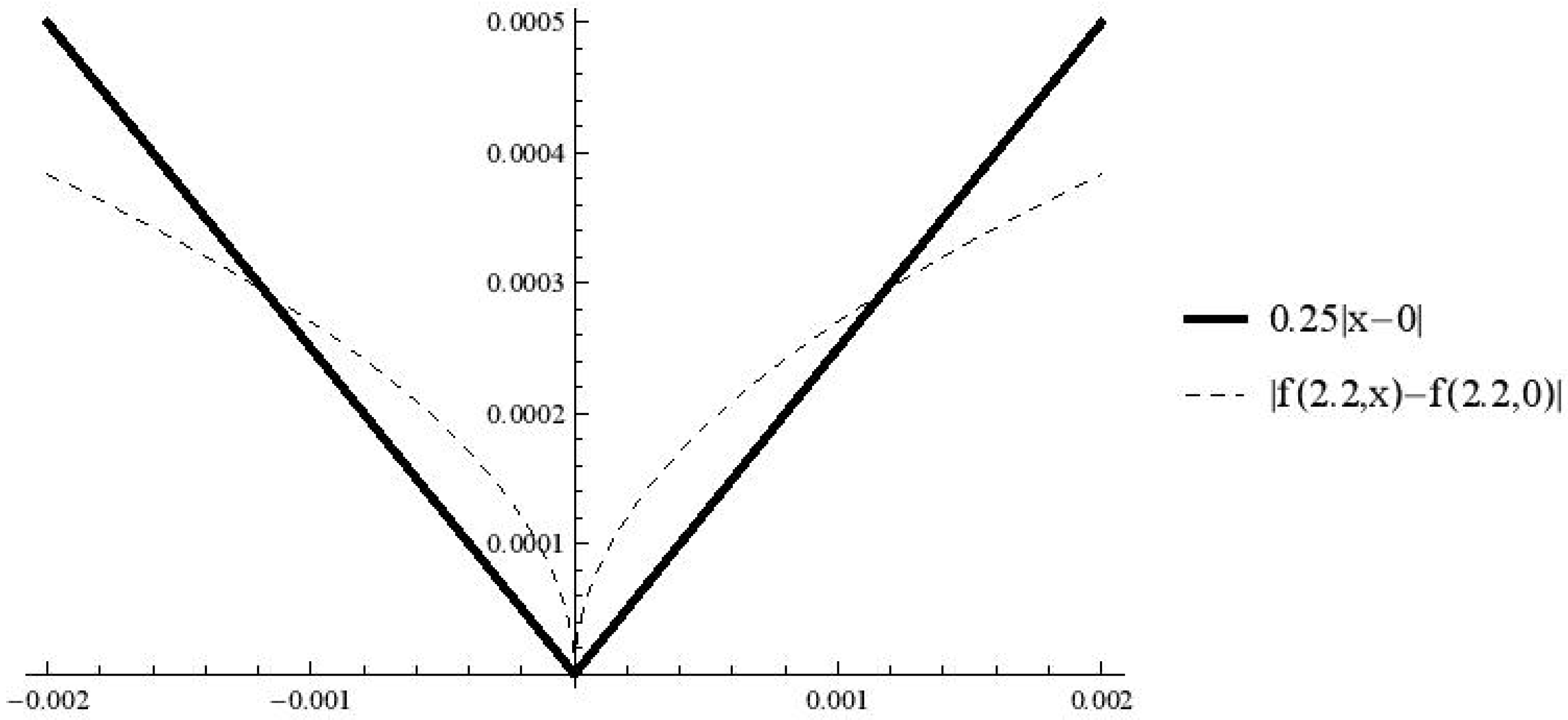
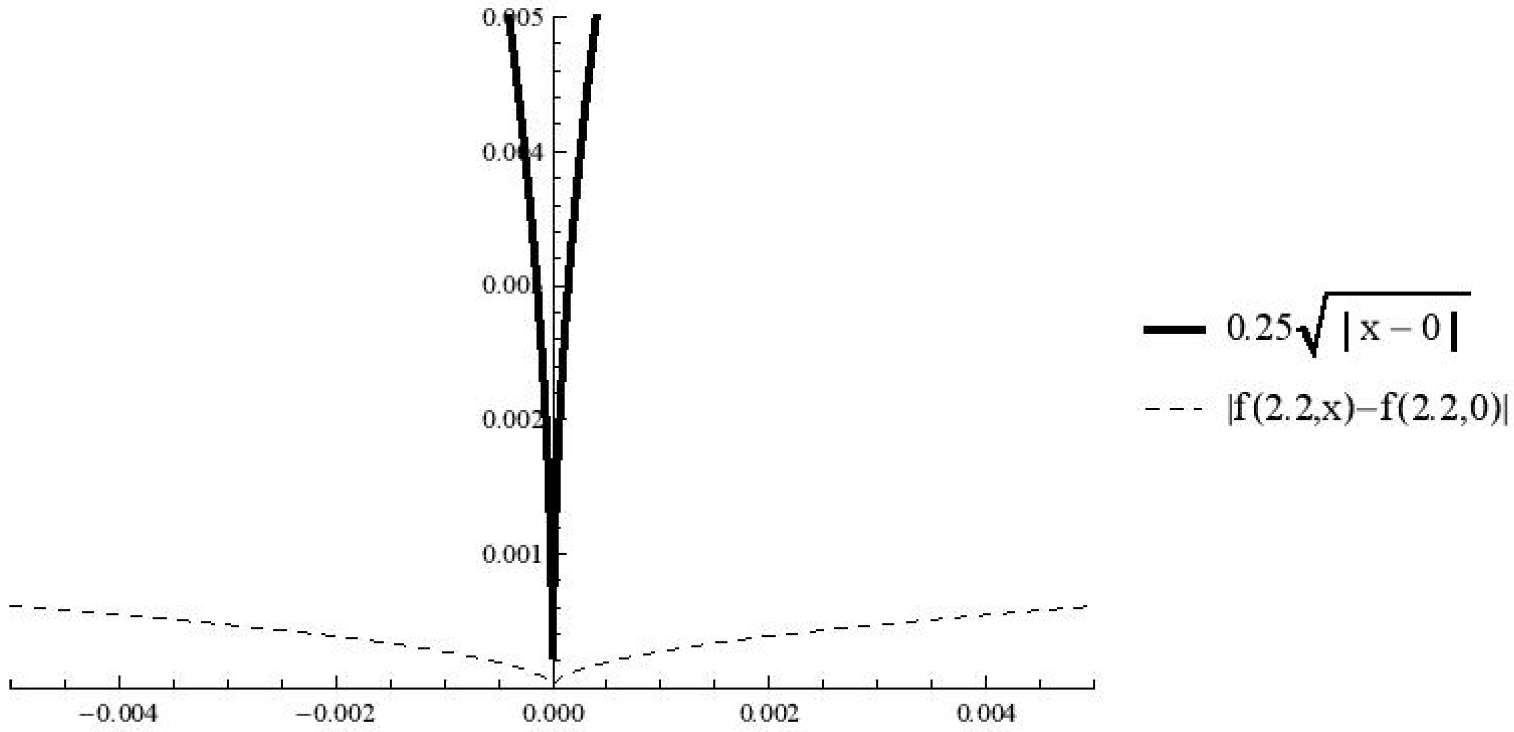
Remark 3.

Note that the boundary value problem (33) and (34) is studied in [25], but the absolute value is missing under the square root. Also, the function $f(t,x)$ is assumed as Lipschitz, but it is not (see Figure 1 for the particular value $t=2.2\in (2,3)$). At the same time the function $f(t,x)$ satisfies the condition 1 with $k=0.25$ (see Figure 2 for the particular value $t=2.2\in (2,3)$), and by one of the fixed point theorems proved in this paper the existence of the solution follows.

5. Discussion

In fixed point theory, the contractive inequality and underlying space play a significant role. A pioneer result in this theory is a Banach contraction principle that consists of compete metric space ($\Omega ,\omega$) as underlying space and the following contractive inequality:

$$\omega (\mathcal{J}(\mathfrak{l}),\mathcal{J}(\kappa ))\le \pi \omega (\mathfrak{l},\kappa )$$

(35)

in which $\mathcal{J}$ is a self mapping and $\pi \in [0,1).$ Over the years, many mathematicians have generalized and extended above contractive inequality in different ways.

In 2012, Wardowski ([10]) initiated the application of a mapping $\mathcal{J}:(\Omega ,\omega )\to (\Omega ,\omega )$ and $\pi >0$ such that:

$$\omega (\mathcal{J}(\mathfrak{l}),\mathcal{J}(\kappa ))>0⟹\pi +\vartheta \left(\omega (\mathcal{J}(\mathfrak{l}),\mathcal{J}(\kappa ))\right)\le \vartheta \left(\omega (\mathfrak{l},\kappa )\right)$$

(36)

for $\mathfrak{l},\kappa \in \Omega$, where $\vartheta :(0,+\infty )\to \mathbb{R}$ satisfies the following conditions:

• $\vartheta (\mathfrak{l})<\vartheta (\kappa )$ for $0<\mathfrak{l}<\kappa$;
• For $\left\{{\mathfrak{l}}_j\right\}\subseteq (0,+\infty )$, ${lim}_{j\to \infty }{\mathfrak{l}}_j=0$ iff ${lim}_{j\to \infty }\vartheta ({\mathfrak{l}}_j)=-\infty ;$
• There exists $0<k<1$ such that ${lim}_{\mathfrak{l}\to 0^{+}}{\mathfrak{l}}^k\vartheta (\mathfrak{l})=0$.

As it is pointed out in [10] the introduced mapping and inequality (36) are a generalization of Banach contraction (35) with $\vartheta (\mathfrak{l})=ln(\mathfrak{l})$, for $\mathfrak{l}>0$.

In this paper, we generalized the mapping used in [10] by introducing two new notions ($\alpha ,\beta$)-type $\vartheta$-contraction and ($\alpha ,\beta$)-type rational $\vartheta$-contraction.

As a partial case of some of our results, we obtained known results in the literature. For example, if $\alpha (\mathfrak{l},\kappa )=\beta (\mathfrak{l},\kappa )=1$ in Theorem 2 then we obtain Theorem 1 ([10]) by which one can derive the result of [1].

6. Conclusions

In the present paper, we introduced two new types of contractions: ($\alpha$,$\beta )$-type $\vartheta$-contraction and ($\alpha$,$\beta )$-type rational $\vartheta$-contraction. Based on their applications we proved new fixed points theorems. These results generalized some known ones from fixed point theory. To support our results, we provided two non trivial examples. The obtained results are noteworthy contributions to the current results of literature in the theory of fixed points. In this field, one can establish ($\alpha$,$\beta )$-type $\vartheta$-contraction and ($\alpha$,$\beta )$-type rational $\vartheta$-contraction for the multivalued mappings in the perspective of complete metric spaces and generalized metric spaces. To illustrate the application of the new fixed point theorems, we considered an integral boundary value problem for a Caputo fractional scalar equation of order from the interval (1,2) and proved the existence of the solution.

References

- Banach, S. Sur les opérations dans les ensembles abstraits et leur applications aux équations intégrales. Fund. Math. 1922, 3, 133–181. [Google Scholar] [CrossRef]
- Boyd, D.W.; Wong, J.S.W. On nonlinear contractions. Proc. Am. Math. Soc. 1969, 20, 458–464. [Google Scholar] [CrossRef]
- Samet, B.; Vetro, C.; Vetro, P. Fixed point theorem for α−ψ contractive type mappings. Nonlinear Anal. 2012, 75, 2154–2165. [Google Scholar] [CrossRef] [Green Version]
- Salimi, P.; Vetro, C.; Vetro, P. Fixed point theorems for twisted (α, β)−ψ-contractive type mappings and applications. Filomat 2013, 27, 605–615. [Google Scholar] [CrossRef] [Green Version]
- Ahmad, J.; Al-Rawashdeh, A.; Azam, A. Fixed point results for {α,ξ}-expansive locally contractive mappings. J. Ineq. Appl. 2014, 2014, 364. [Google Scholar] [CrossRef] [Green Version]
- Asl, J.H.; Rezapour, S.; Shahzad, N. On fixed points of α−ψ contractive multifunctions. Fixed Point Theory Appl. 2012, 2012, 212. [Google Scholar] [CrossRef] [Green Version]
- Hussain, H.; Ahmad, J.; Azam, A. Generalized fixed point theorems for multi-valued α−ψ-contractive mappings. J. Ineq. Appl. 2014, 2014, 348. [Google Scholar] [CrossRef] [Green Version]
- Kutbi, M.A.; Ahmad, J.; Azam, A. On fixed points of α−ψ-contractive multi-valued mappings in cone metric spaces. In Abstract and Applied Analysis; Hindawi: Warsaw, Poland, 2013; p. 313782. [Google Scholar]
- Salimi, P.; Latif, A.; Hussain, N. Modified α−ψ-contractive mappings with applications. Fixed Point Theory Appl. 2013, 2013, 151. [Google Scholar] [CrossRef] [Green Version]
- Wardowski, D. Fixed points of a new type of contractive mappings in complete metric spaces. Fixed Point Theory Appl. 2012, 2012, 94. [Google Scholar] [CrossRef] [Green Version]
- Wardowski, D.; Van Dung, N. Fixed points of F-weak contractions on complete metric spaces. Demonstr. Math. 2014, 47, 146–155. [Google Scholar] [CrossRef]
- Kaddouri, H.; Huseyin, I.; Beloul, S. On new extensions of F-contraction with application to integral inclusions. UPB Sci. Bull. Ser. A 2019, 81, 31–42. [Google Scholar]
- Arshad, M.; Khan, S.; Ahmad, J. Fixed Point Results for F-contractions involving some new rational expressions. JP J. Fixed Point Theory Appl. 2016, 11, 79–97. [Google Scholar] [CrossRef]
- Ahmad, J.; Al-Rawashdeh, A.; Azam, A. New Fixed Point Theorems for Generalized F-Contractions in Complete Metric Spaces. Fixed Point Theory Appl. 2015, 2015, 80. [Google Scholar] [CrossRef] [Green Version]
- Ahmad, J.; Aydi, H.; Mlaiki, N. Fuzzy fixed points of fuzzy mappings via F-contractions and an applications. J. Intell. Fuzzy Syst. 2019, 37, 5487–5493. [Google Scholar] [CrossRef]
- Al-Mazrooei, A.E.; Ahmad, J. Fuzzy fixed point results of generalized almost F-contraction. J. Math. Comput. Sci. 2018, 18, 206–215. [Google Scholar] [CrossRef]
- Shahzad, M.I.; Al-Mazrooei, A.E.; Ahmad, J. Set-valued G-Prešić type F-contractions and fixed point theorems. J. Math. Anal. 2019, 10, 26–38. [Google Scholar]
- Al-Mezel, S.A.; Ahmad, J. Generalized fixed point results for almost (α, Fσ)-contractions with applications to Fredholm integral inclusions. Symmetry 2019, 11, 1068. [Google Scholar] [CrossRef] [Green Version]
- Abdou, A.N.A.; Ahmad, J. Multivalued fixed point theorems for ϑρ-contractions with applications to Volterra integral inclusion. IEEE Access 2019, 7, 146221–146227. [Google Scholar] [CrossRef]
- Altun, G.; Mınak, G.; Dag, H. Multivalued F-contractions on complete metric space. J. Nonlinear Convex Anal. 2015, 16, 659–666. [Google Scholar]
- Cosentino, M.; Vetro, P. Fixed point results for F-contractive mappings of Hardy-Rogers-type. Filomat 2014, 28, 715–722. [Google Scholar] [CrossRef] [Green Version]
- Hussain, N.; Ahmad, J.; Azam, A. On Suzuki-Wardowski type fixed point theorems. J. Nonlinear Sci. Appl. 2015, 8, 1095–1111. [Google Scholar] [CrossRef]
- Budhia, L.B.; Kumam, P.; Martínez-Moreno, J.; Gopal, D. Extensions of almost-F and F-Suzuki contractions with graph and some applications to fractional calculus. Fixed Point Theory Appl. 2016, 2016, 2. [Google Scholar] [CrossRef] [Green Version]
- Gopal, D.; Abbas, M.; Patel, D.K.; Vetro, C. Fixed points of α-type F-contractive mappings with an application to nonlinear fractional differential equation. Acta Math. Sci. 2016, 36, 957–970. [Google Scholar] [CrossRef]
- Mehmood, N.; Ahmad, N. Existence results for fractional order boundary value problem with nonlocal non-separated type multi-point integral boundary conditions. AIMS Math. 2019, 5, 385–398. [Google Scholar] [CrossRef]
- Ahmad, B.; Alsaedi, A.; Alsharif, A. Existence results for fractional-order differential equations with nonlocal multi-point-strip conditions involving Caputo derivative. Adv. Diff. Eq. 2015, 348. [Google Scholar] [CrossRef] [Green Version]
- Liu, W.; Zhuang, H. Existence of solutions for Caputo fractional boundary value problems with integral conditions. Carpathian J. Math. 2017, 33, 207–217. [Google Scholar]
- Kilbas, A.A.; Srivastava, H.M.; Trujillo, J.J. Theory and Applications of Fractional Differential Equations; Elsevier: Amsterdam, The Netherlands, 2006. [Google Scholar]
Figure 1.
Graphs of and .
Figure 2.
© 2020 by the authors. Licensee MDPI, Basel, Switzerland. This article is an open access article distributed under the terms and conditions of the Creative Commons Attribution (CC BY) license (http://creativecommons.org/licenses/by/4.0/).
Share and Cite
MDPI and ACS Style
Zahed, H.; Fouad, H.A.; Hristova, S.; Ahmad, J. Generalized Fixed Point Results with Application to Nonlinear Fractional Differential Equations. Mathematics 2020, 8, 1168. https://doi.org/10.3390/math8071168
AMA Style
Zahed H, Fouad HA, Hristova S, Ahmad J. Generalized Fixed Point Results with Application to Nonlinear Fractional Differential Equations. Mathematics. 2020; 8(7):1168. https://doi.org/10.3390/math8071168
Chicago/Turabian StyleZahed, Hanadi, Hoda A. Fouad, Snezhana Hristova, and Jamshaid Ahmad. 2020. "Generalized Fixed Point Results with Application to Nonlinear Fractional Differential Equations" Mathematics 8, no. 7: 1168. https://doi.org/10.3390/math8071168
Note that from the first issue of 2016, this journal uses article numbers instead of page numbers. See further details here.