Article

Monitoring Excess Exposure to Air Pollution for Professional Drivers in London Using Low-Cost Sensors

by
Louise Bøge Frederickson
1,2,
Shanon Lim
3,
Hugo Savill Russell
1,2,4,5,
Szymon Kwiatkowski
2,
James Bonomaully
2,
Johan Albrecht Schmidt
2,
Ole Hertel
4,5,
Ian Mudway
3,
Benjamin Barratt
3 and
Matthew Stanley Johnson
1,2,*
1
Department of Chemistry, University of Copenhagen, DK-2100 Copenhagen, Denmark
2
AirLabs Denmark, Nannasgade 28, DK-2200 Copenhagen, Denmark
3
Environmental Research Group, MRC Centre for Environment and Health, Imperial College London, London SW7 2BU, UK
4
Department of Environmental Science, Aarhus University, DK-4000 Roskilde, Denmark
5
Danish Big Data Centre for Environment and Health (BERTHA), Aarhus University, DK-4000 Roskilde, Denmark
*
Author to whom correspondence should be addressed.
Atmosphere 2020, 11(7), 749; https://doi.org/10.3390/atmos11070749
Submission received: 12 June 2020 / Revised: 11 July 2020 / Accepted: 12 July 2020 / Published: 15 July 2020
(This article belongs to the Section Air Quality)

Abstract

:
In this pilot study, low-cost air pollution sensor nodes were fitted in waste removal trucks, hospital vans and taxis to record drivers’ exposure to air pollution in Central London. Particulate matter (PM 2.5 and PM 10 ), CO 2 , NO 2 , temperature and humidity were recorded in real-time with nodes containing low-cost sensors, an electrochemical gas sensor for NO 2 , an optical particle counter for PM 2.5 and PM 10 and a non-dispersive infrared (NDIR) sensor for CO 2 , temperature and relative humidity. An intervention using a pollution filter to trap PM and NO 2 was also evaluated. The measurements were compared with urban background and roadside monitoring stations at Honor Oak Park and Marylebone Road, respectively. The vehicle records show PM and NO 2 concentrations similar to Marylebone Road and a higher NO 2 -to-PM ratio than at Honor Oak Park. Drivers are exposed to elevated pollution levels relative to Honor Oak Park: 1.72 μ g m 3 , 1.92 μ g m 3 and 58.38 ppb for PM 2.5 , PM 10 , and NO 2 , respectively. The CO 2 levels ranged from 410 to over 4000 ppm. There is a significant difference in average concentrations of PM 2.5 and PM 10 between the vehicle types and a non-significant difference in the average concentrations measured with and without the pollution filter within the sectors. In conclusion, drivers face elevated air pollution exposure as part of their jobs.

1. Introduction

Traffic-related air pollution has a disproportionate local effect on passengers and drivers, cyclists and pedestrians and residents in areas with a high traffic density [1]. Professional drivers are particularly at risk due to the amount of time spent inside vehicles in traffic [2]. Exposure to air pollution is associated with a wide range of adverse health effects such as asthma, cardiovascular problems, inflammatory blood markers, adverse respiratory events and lung cancer, resulting in increased mortality rates [3,4,5]. Drivers and passengers are exposed to high levels of various air pollutants such as particulate matter (PM), volatile organic compounds (VOCs), semi-volatile organic compounds (SVOCs), carbon monoxide (CO) and oxides of nitrogen (NO x ), originating from vehicle emissions and regional sources [6]. There are several factors affecting in-cabin air pollutants concentrations, such as driving conditions, traffic volume, the type, age and conditions of vehicles, cabin ventilation settings, commuting distance, vehicle speed, air exchange rate and driving route types [7].
Several studies have shown that air pollution exposure is higher for people inside a vehicle cabin than for cyclists or pedestrians outside, within or near high traffic locations [8,9,10,11,12]. Personal exposure studies have shown that pollution exposure is highest when people are commuting. While most people only commute one to two hours per day, it is likely that those that are required to work in this environment are disproportionately affected by high air pollution exposure [13,14]. The interior of a vehicle is a challenging environment for air pollution field studies due to spatial requirements, vibration, noise and variable temperature [13,14,15]. However, due to recent improvements in sensor technologies and testing designs, more in-cabin air quality measurement studies are being published [7,16,17,18].
There is significant interest in using low-cost sensors to characterize personal exposure by measuring pollution concentrations in micro-environments in which people spend time, such as the workplace, at home and in various means of transport used during commuting [19]. Combining the different pollution sensors into a node (with signal processing and communication, as well as data storage and analysis) forms a useful tool to assess air quality. These sensor nodes are typically characterized by their small size and weight, relatively short response time and low power requirements [20,21,22]. Low-cost sensors have developed rapidly in recent years and are changing the paradigm of air pollution monitoring beyond the geographically restricted roadside and background monitoring accomplished by dedicated stations. The high time resolution of the components, combined with the large data throughput and the high spatial resolution made possible by multiple installations, allows researchers to achieve a more comprehensive understanding of an individual’s true exposure [20,23,24]. While low-cost sensors are not yet likely to substitute accredited routine monitoring instruments at fixed-site monitoring stations for the accurate measurements of well-mixed gases in the atmosphere, they are particularly useful for measurements of short-lived pollutants with sources located inside cities. Thus, they can supplement the conventional monitoring station networks and increase the spatio-temporal resolution of measurements [15,25]. In addition, their small size enables the monitoring of personal exposure; for example, at home, at work and during transit [26].
Recent advances in research related to in-vehicle air pollution exposure have led to several innovations in this field. In modern vehicles, for example, a coarse particle filter is built into the ventilation system. However, such filters are typically not designed to remove gas-phase chemicals or fine particulate matter, which have been associated with negative health effects [27]. Specially designed aftermarket filters including activated carbon have become available as in-cabin air cleaners.
The main purpose of this pilot study is to characterize multiple-pollution exposures of professional drivers in three different sectors in Central London in the UK. Measurements were made in real time using a low-cost sensor, AirNode Generation One (AGO by AirLabs), which contains an electrochemical, gas sensor (NO 2 ), an optical particle counter (PM 2.5 , PM 10 ) and a non-dispersive infrared (NDIR) sensor (CO 2 ) including sensors for temperature (T) and relative humidity (RH). The low-cost sensors were mounted in 14 vehicles (three waste removal trucks, seven hospital transport vans and four taxis) of varying types, ages and mileages. The number of passengers and the state of the vehicles’ ventilation systems, windows and doors also varied. In addition, the effect of an in-cabin Air Filtration System (AFS by AirLabs) using a fine particle filter and activated charcoal, chemically modified to increase its affinity for NO 2 , was tested under these real-world conditions. The AGO was validated against a reference monitoring station and AFS was tested in the laboratory as well as in the field. This study assesses the in-cabin concentrations of PM 2.5 , PM 10 , NO 2 , and CO 2 across a range of vehicles and operating conditions. To the author’s knowledge, this paper is the first to measure multiple pollutant exposures in the real-world professional driving settings using low-cost sensors. In addition, this study tests the utility of the AGO in the field as part of an intervention study and therefore contributes information that is essential to the development of robust protocols in this area.

2. Materials and Methods

This study is approved by the ethics committee at the University of Copenhagen (Journal no. 504-0104/19-5000). The following section describes the key components of the AGO, its validation against a reference monitoring station, the laboratory tests of the AFS and the field study design of the exposure campaigns.

2.1. Description of the Sensor Node, AGO

The AGOs used in the vehicles are compact, low-cost, portable air quality monitoring devices with dimensions of 88 × 88 × 90 mm. The devices are assembled by AirLabs into weatherproof enclosures with full exposure to ambient air. Each device includes sensors for measuring PM 2.5 and PM 10 (SDS-011 from Nova Fitness Co., Ltd.: Jinan, China), NO 2 (NO2B43F from Alphasense Ltd.: Braintree, UK), and CO 2 , T and RH (SCD30 from Sensirion: Stäfa, Switzerland) at a 1 min time resolution. The AGO is powered by the vehicle’s battery using a USB cable, has integrated telemetry and automatically reports measurements to the AirLabs Cloud hosted by Amazon Web Services (AWS). In addition, each node is equipped with a control board and micro-controller unit (ESP32) to program the sensors.
The SDS-011 sensor [28] is an air quality sensor used for measuring PM based on light scattering [29], where particle density distribution is determined using the intensity distribution patterns produced when particles scatter a laser beam [30]. The sensor module includes a fan to ensure a continuous flow of air through the sensor chamber [31]. An algorithm converts the particle density distribution into particle mass [32]. The sensor has a resolution of 0.3 μ g m 3 and a response time of 10 s [33,34,35,36].
For NO 2 measurements, the NO2B43F sensor [37] is used. This is an amperometric electrochemical gas sensor containing four electrodes, where the working principle is based on electrochemistry [19]. The target gas enters the working electrode by diffusion, where it is chemically reduced, resulting in a current signal. The counter electrode balances the current, and the reference electrode sets the operating potential of the working electrode. The fourth electrode is auxiliary and compensates for baseline changes in the sensor. An individual sensor board is used to guarantee a low-noise environment and optimize the sensor resolution for low parts per billion (ppb) levels. The electrochemical sensor generates a current proportional to the NO 2 concentration. A trans-impedance amplifier converts the current from the electrochemical cell into a voltage. The voltage is amplified further by a non-inverting operational amplifier; then, a 16-bit analogue to digital (A/D) converter (ADS1115) samples the output and produces a digital reading of the voltage level. This is used by the microprocessor to calculate the actual gas concentration [38,39,40]. To minimize possible cross-interference from ozone, the NO 2 sensors were fitted with integrated catalytic ozone filters. The performance of these filters was verified in the laboratory, and the NO 2 sensors showed no significant response to ozone in the range of 0–100 ppb. Cross-interferences from other common gas pollutants were not considered important based on prior studies [40,41].
The SCD30 sensor [42] measures CO 2 using non-dispersive infrared (NDIR) spectroscopy [43]. Temperature and relative humidity sensors are integrated into the same module [44]. The sensors are calibrated at the factory [45]. The main characteristics of the sensing elements are summarized in Table 1.

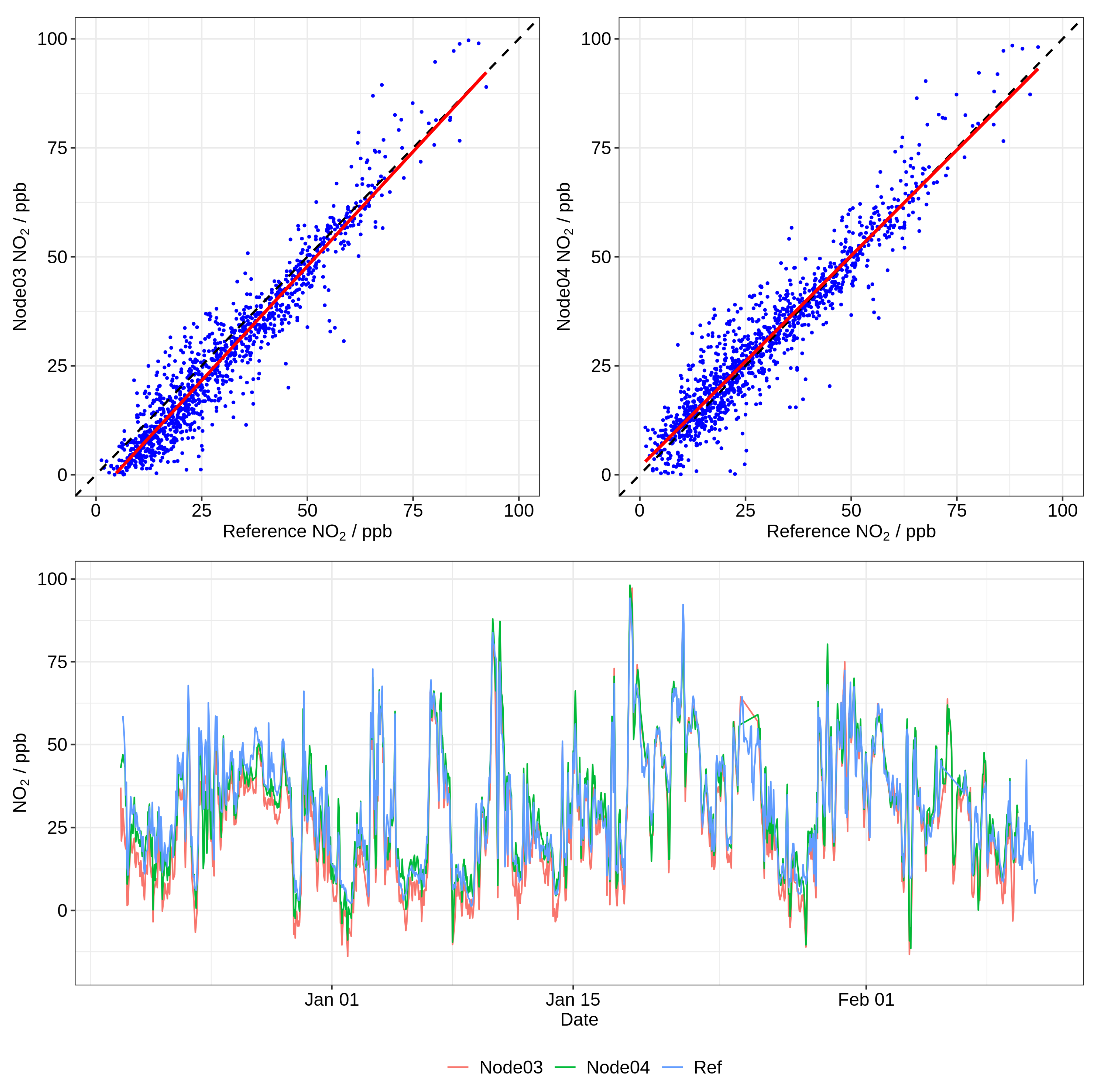
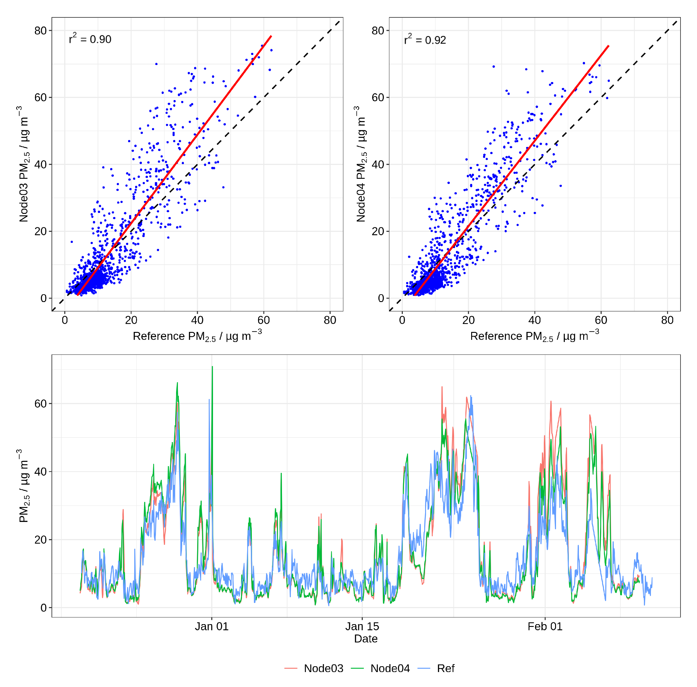
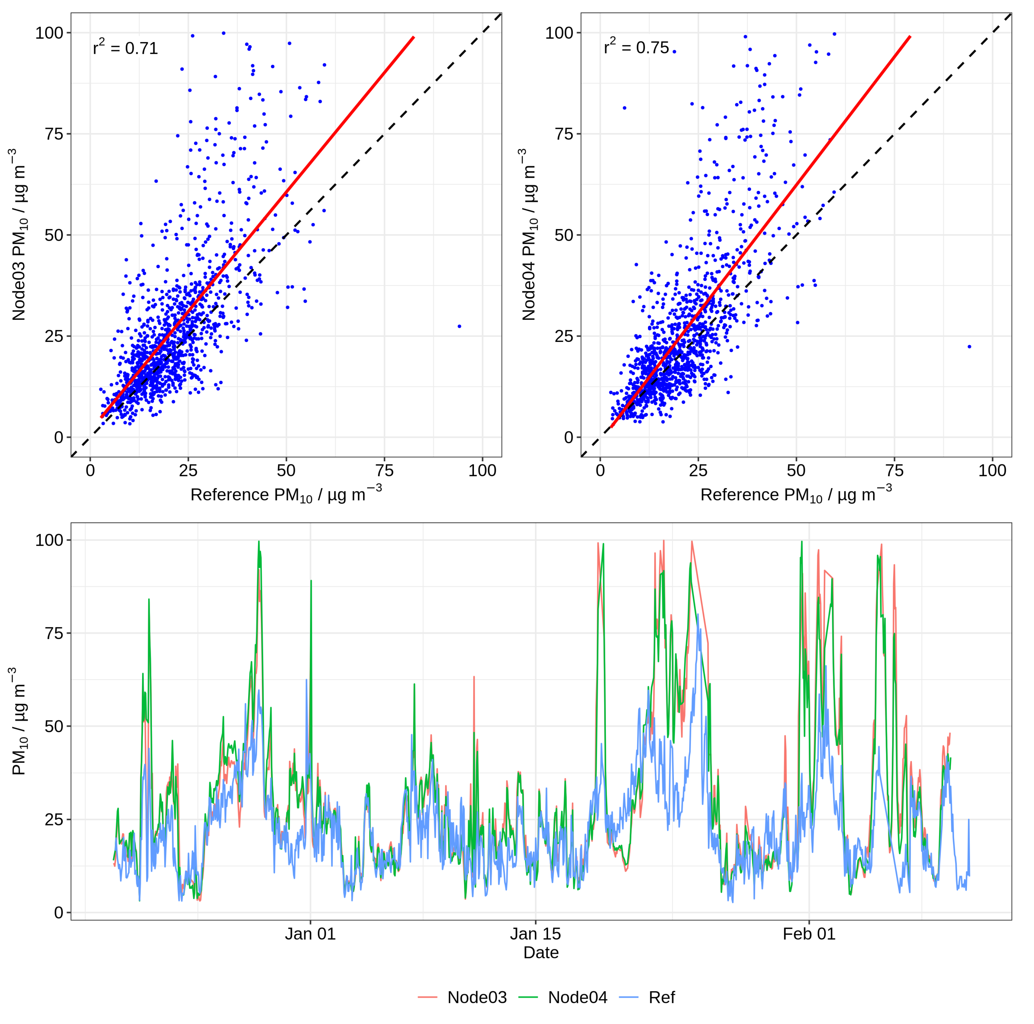
2.2. Field Calibration of the Sensor Node

The performance of the AGO for PM 2.5 , PM 10 and NO 2 was established by co-locating the nodes with a reference monitoring station. Validation was performed from December 2017 to February 2018 by co-locating the AGO at District of Columbia Municipal Regulations’ (DCMR) Schiedam air quality monitoring station in Rotterdam, the Netherlands. The concentration of NO 2 was measured by a reference standard chemiluminescence NOx analyzer, and concentrations of PM were measured by a Met-One BAM 1020. Measurement conditions ranged from 30% to 70% RH and −0.2 to 17.5 °C. The time series and the correlation plots of the reference NO 2 concentrations and the NO 2 concentrations measured by Node03 and Node04 are shown in Figure 1. The linear regression fit (solid red line) and a 1:1 line (dashed black line) are shown for both sensor nodes in the scatter plots. Correlation plots and time series plot for PM 2.5 and PM 10 concentrations are seen in Appendix A, Figure A1 and Figure A2. The performance metrics for PM 2.5 , PM 10 and NO 2 are presented in Table 2. The high correlation coefficients ( r 2 = 0.90–0.96) for PM 2.5 and NO 2 and moderate correlation coefficient ( r 2 = 0.71–0.75) for PM 10 indicate that the AGOs are capable of capturing the variability in pollutant concentrations despite wide variations in ambient temperature and relative humidity over the monitoring period.

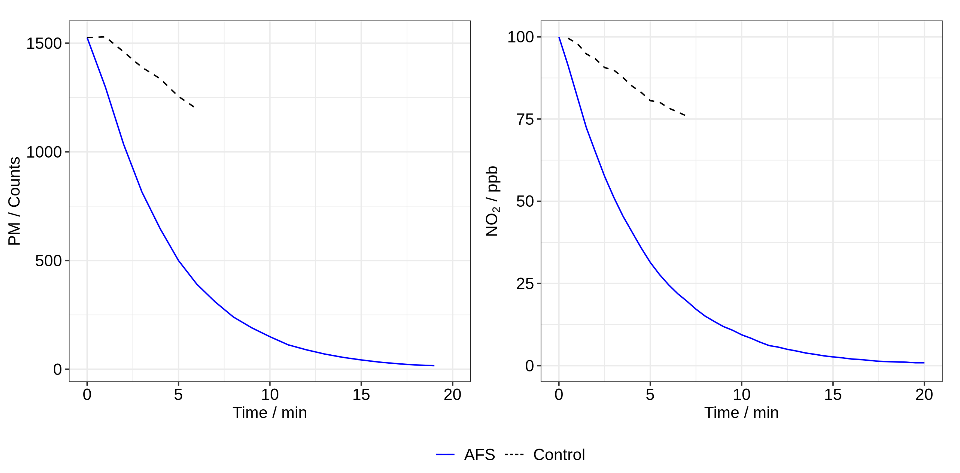
2.3. Lab Testing of the Air Filtration System

The Air Filtration System (AFS by AirLabs) was tested under controlled settings using a cuboid chamber with a volume of 2 m 3 , representative of the volume of the cabin in a typical car. A mixing fan inside the chamber allows the homogenization of pollutant levels. NO 2 was introduced into the chamber via a mass flow controller (SLA5800, 0 to 100 mL/min range, Brooks Instruments: Hatfield, PA, USA), from a calibrated gas mixture (NO 2 mole fraction 0.00982 ± 0.00002 in nitrogen, Praxair Norge AS: Oslo, Norway). NO 2 concentrations were measured using a chemiluminescence monitor (Thermo Scientific Model 42i, Thermo Fisher Scientific Inc.: Waltham, MA, USA) operated with a particle filter at its inlet. For PM, an internal combustion standard was used to produce size distributions comparable to those found in traffic. Particles with an aerodynamic diameter of 0.3 μ m are used to quantify the performance. The particles were measured using a scanning mobility particle sizer (TSI Model 3080 Electrostatic Classifier (TSI Incorporated: Shoreview, MN, USA) with TSI Model 3081 Long DMA and TSI CPC model 3772). The AFS was placed in the chamber with ambient air at 22 °C, and an aliquot of NO 2 or PM was introduced into the chamber with mixing fan turned on. The concentrations in the chamber were monitored for an initial 10 min period to determine background removal due to air exchange and adsorption onto the walls. Then, the AFS was turned on and the concentrations monitored until the background concentration was reached.
Figure 2 shows the removal of PM with an aerodynamic diameter of 0.3 μ m (left) and NO 2 (right) by the AFS (solid blue line). The black dashed line is the control, which was obtained by observing the pollutants’ behavior in the chamber without the AFS in operation. For the easy comparison of the control and the removal by AFS, the starting concentrations were scaled to start at the same concentration. Even though the AFS was switched off, pollutants were still removed due to aggregation and adsorption on the walls of the chamber, and 20% of NO 2 and PM (d = 0.3 μ m) was removed within 5 min. When the AFS was turned on, a more rapid removal was seen, with a removal of 63% of the starting PM (d = 0.3 μ m) and NO 2 concentrations within 4.5 and 6 min, respectively. These experiments only measured PM with a diameter of 0.3 μ m, but the AFS removes particles of a wide range of sizes. Particles with a diameter of 0.3 μ m are close to the most penetrating particle size, so both larger and smaller particles are removed more effectively, and so this can be considered the lower limit for removal efficiency.

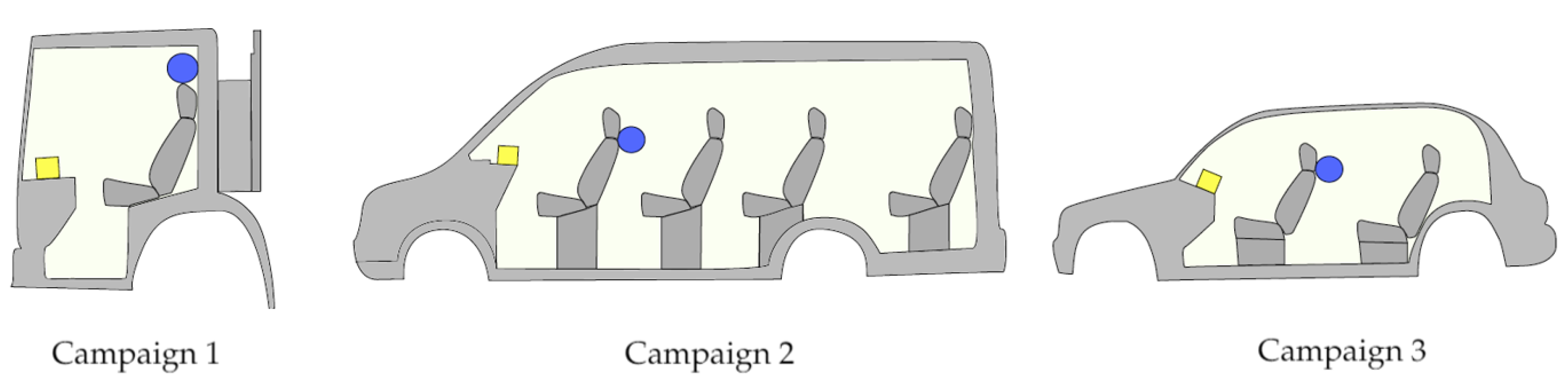
2.4. Field Study Design

The driver exposure campaigns were conducted between August and October of 2019 (with a total of 56 days of sampling) in Central London, the United Kingdom. The air pollution concentrations were monitored during work hours using 14 different vehicles. The vehicles were divided into three campaigns: waste removal trucks, hospital vans (including shuttle buses and ambulances) and taxis. The characteristics of the different campaigns are summarized in Table 3.
All in-vehicle monitoring was conducted with the heating, ventilation and air conditioning (HVAC) set to suit the driver’s comfort. The drivers were asked to keep the windows closed if possible when the in-cabin filter was turned on. There was no noticeable difference in vehicle size or cabin volume between the vehicles used within a given class. However, the interior volumes spanned a factor of four from approximately 2 to 8 m 3 between the different campaigns, with waste removal trucks at 2 m 3 and shuttle buses at 8 m 3 . The size differences are illustrated in Figure 3. All vehicles were equipped with an AGO to measure the driver’s exposure to air pollution in real-time. The AGO was placed on the dashboard in front of the passenger seat. In addition, vehicles were provided an AFS for the reduction of PM and NO 2 , which was positioned behind the driver’s headrest. For each vehicle, four days of measuring were conducted; two days with the AFS turned on and two days with the AFS turned off. The drivers were responsible for starting both devices when their shift started.
Statistical analysis was performed using the non-parametric Wilcoxon–Mann–Whitney Rank test (i.e., no assumptions of data distributions such as normality) to compare the differences among measured pollutant concentrations between driving sectors and with and without the AFS. The statistical significance was assumed at the 5% level (p < 0.05).

3. Results and Discussion

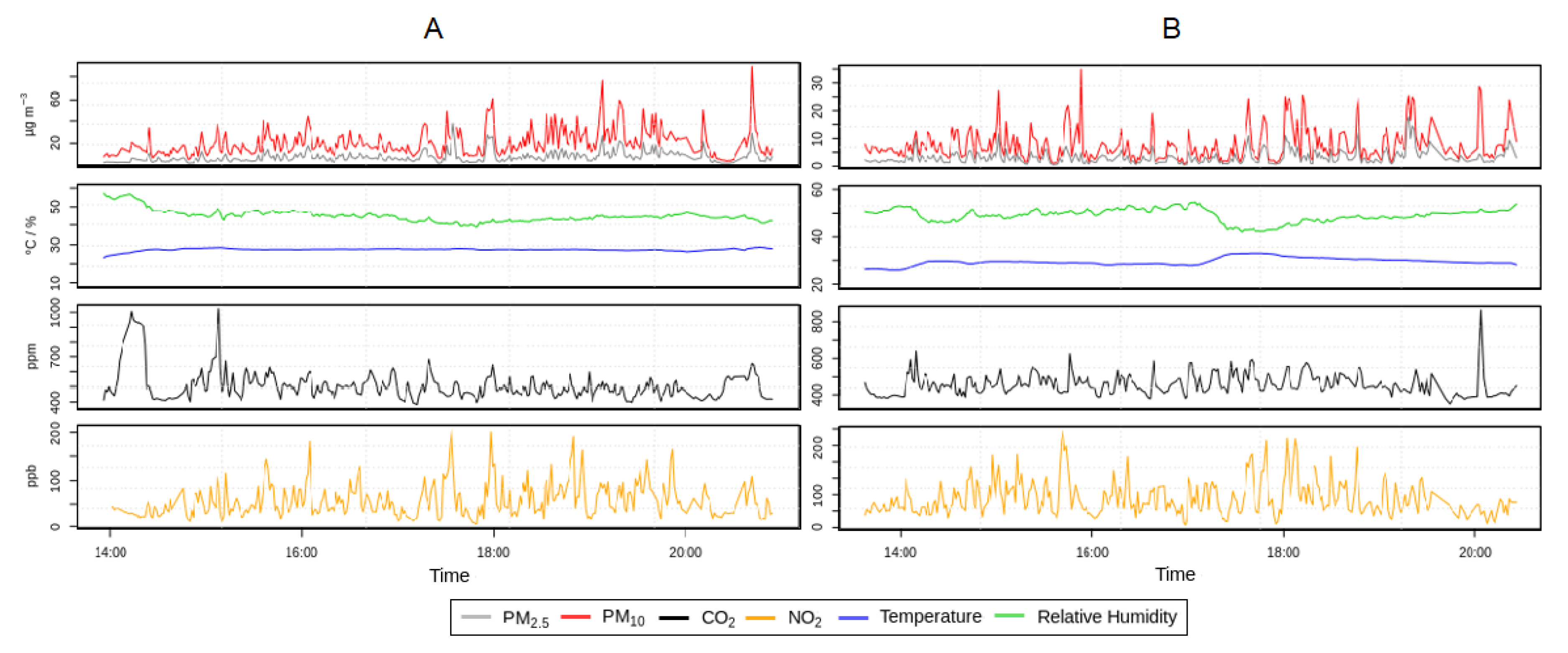
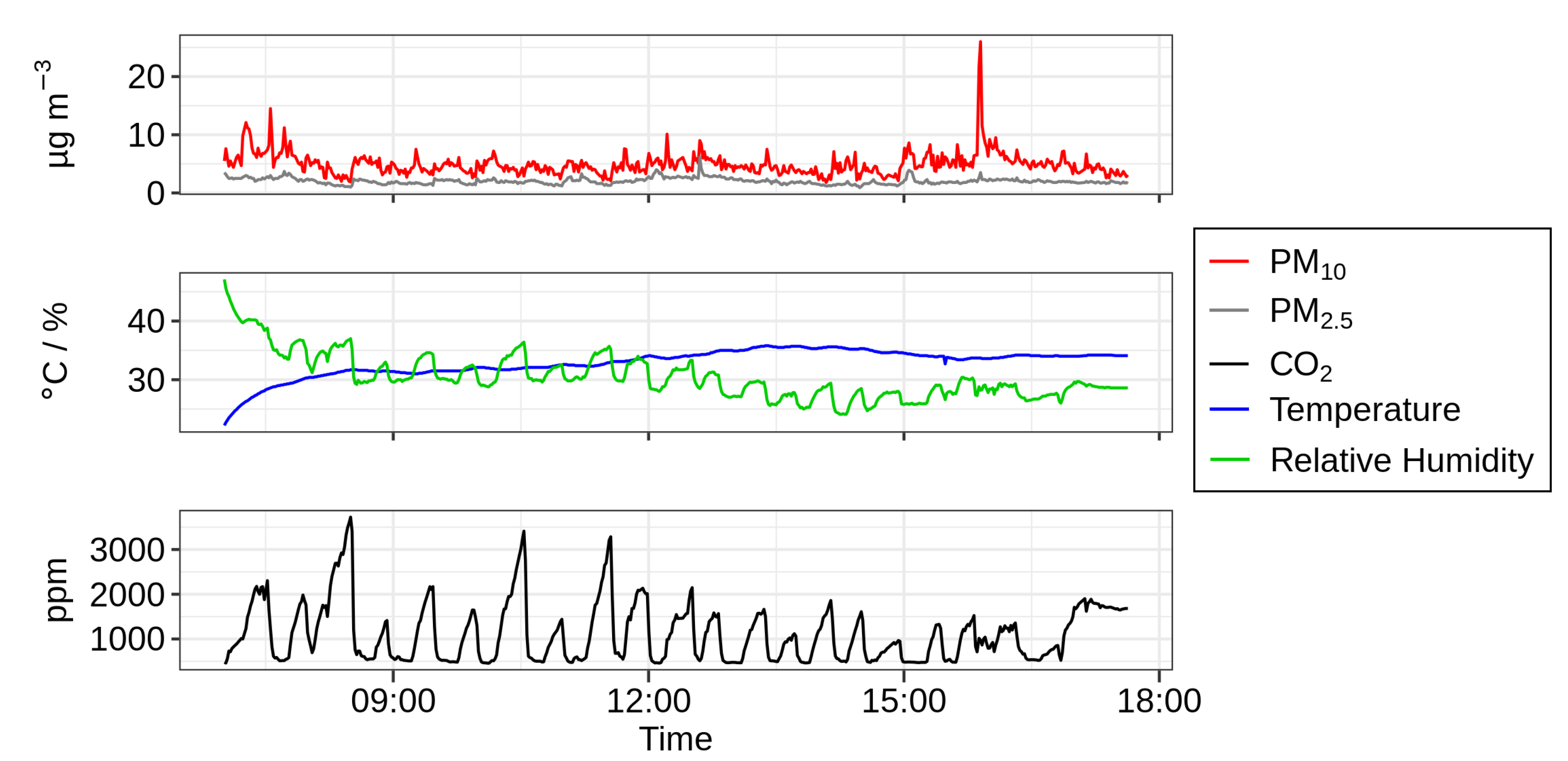
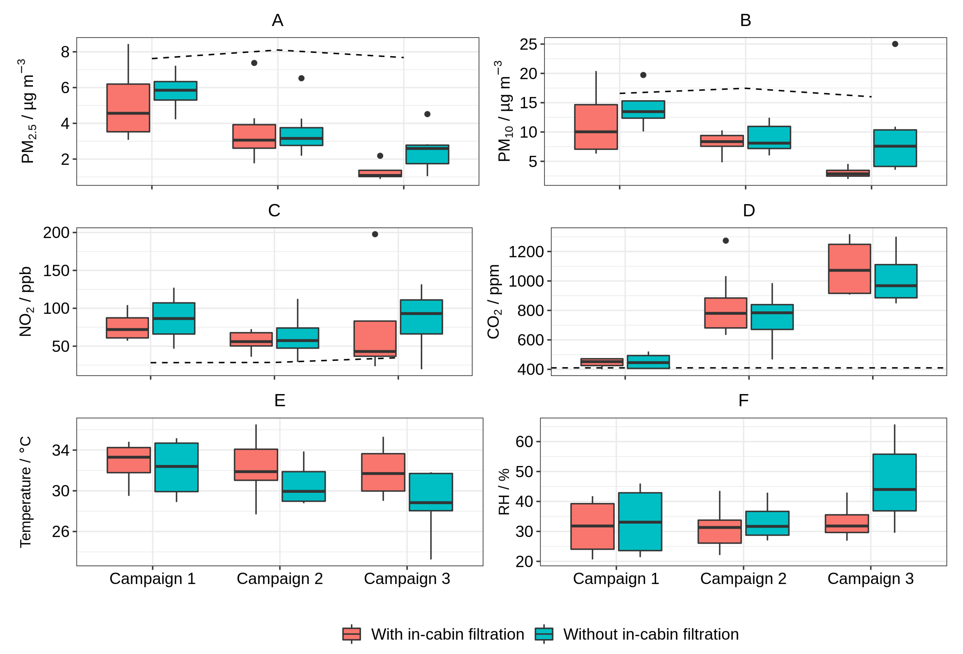
3.1. Driver Exposure Campaigns

In total, 14 vehicles were monitored over 56 working days throughout the study period. Data from six of the days were excluded because the time series were interrupted due to technical problems, the disruption of communication or AGO handling errors. For each day, the pollutants and in-cabin conditions (temperature and relative humidity) were averaged and a standard deviation was determined; see Table A1. During monitoring, the average in-cabin temperature ranged from 11 to 49 °C (average = 32.1 °C), and the average in-cabin relative humidity ranged from 9.4% to 81% (average = 31.1%). The high maximum and average temperatures are because direct sunlight hit the AGO during measurements. The data show substantial variability in in-cabin concentrations of all pollutants between sectors, drivers and times and locations, which is due to the changes in traffic density, air exchange rate, meteorology, vehicle operational mode and the air quality of the driving area. The large standard deviations are a result of this variation; for illustration, see Table A1 and Figure 4. In addition, road type and time-of-day had some indirect influence on the in-vehicle pollutant levels.

3.1.1. NO 2 Concentrations

Electrochemical gas sensors take time to stabilize when they are powered up after being switched off for a while. Due to this fact, the data before the point of stabilization were removed from measurements. Approximately 20% of the NO 2 data for each test run were excluded. Furthermore, the sensors could have technical issues, in part due to the difficulty of resolving small changes in electrochemical current ( μ A), leading to the additional exclusion of 5% of the total data. There is a certain uncertainty (15%) regarding the zero-baseline, since the off-sets were adjusted manually.
As shown in Table A1, average NO 2 concentrations were relatively high and had a high variability, ranging from 46.7 to 150.9 ppb for Campaign 1, 29.9 to 113.9 ppb for Campaign 2 and 30.9 to 107.6 ppb for Campaign 3. The large variations in the NO 2 concentrations likely reflect periods when the vehicles were in heavy traffic in Central London. EU guidelines stipulate that ambient NO 2 should not exceed 21 ppb on average annually, or 106 ppb on average over 24 h [46,47]. The results are compared with the reference roadside Urban Atmospheric Observatory placed at Marylebone Road, London. The in-cabin values are higher than at the reference roadside monitor on Marylebone Road, which likely reflects NO 2 gradients between the middle of the road and the roadside monitor.
On some of the days, drivers were exposed to NO 2 levels above the recommended levels for short-term exposure (1 h) of ambient air. The results show periods failing to meet the long-term exposure (1 year) standards; however, none of the drivers are exposed to these levels on an average daily basis over the working year. Although these standards do not apply to occupational exposure and indoor environments, the data still indicate that drivers face health risks. The drivers in all three campaigns were exposed to high levels of NO 2 , in part due to frequent stops involving the opening of the cabin doors. An example of this is shown in Figure 4, which presents in-cabin concentrations of PM 2.5 , PM 10 , NO 2 and CO 2 , as well as temperature and relative humidity for a waste removal truck during working hours (Campaign 1). This reflects exposures to diesel exhaust emissions, so the findings here have direct implications for urban areas throughout Europe due to the high proportion of diesel vehicles in the fleet. It was measured on the 12 (A) and 14 (B) of August; the AFS was only used on the second day. High peaks of NO 2 were associated with local sources and are a proxy for vehicle emissions.

3.1.2. PM Concentrations

Figure 4 shows a time series of in-cabin concentrations for two days of measurements in Campaign 1. Average in-cabin PM concentrations were relatively low with high variability. Average PM 2.5 concentrations for Campaigns 1, 2 and 3 were in the range 2.5 to 8.0 μ g m 3 , 1.1 to 7.3 μ g m 3 and 0.9 to 2.8 μ g m 3 , respectively. Average PM 10 concentrations for Campaigns 1, 2 and 3 were 3.9 to 20.6 μ g m 3 , 3.3 to 11.9 μ g m 3 and 2.8 to 10.5 μ g m 3 , respectively. For comparison, EU guidelines stipulate that ambient PM 2.5 should not exceed 10 μ g m 3 annual average or 25 μ g m 3 24 h average, and that PM 10 should not exceed 20 μ g m 3 annual average or 50 μ g m 3 24 h average [47]. These guidelines do not apply to indoor and work environments; however, they give an indication of the air quality in the work environment. The concentrations of PM were highest in Campaign 1, as seen for NO 2 , due to the type of work and frequent stops with opening doors. While the time-averaged concentrations were below the recommended exposure limits for ambient air, drivers were exposed to transient peaks exceeding these thresholds; see Figure 4. Concentration changes between days in a given campaign were generally within a standard deviation of one another. The PM results were compared with the reference roadside Urban Atmospheric Observatory on Marylebone Road, London. The in-cabin values are lower than those of the roadside monitor, indicating that the built-in filtration system in the vehicles prevents some of the particles from entering the vehicle cabin.
The number of occupants in the vehicles is also an important consideration when interpreting PM 2.5 and PM 10 data, since PM can be re-suspended by human activities [48] and therefore would be expected to be higher on runs with a higher number of occupants and with more activity. For all three campaigns, correlations between PM and CO 2 and RH were investigated. Given the assumption that the more the occupants, the higher the concentration of CO 2 and RH, PM concentrations were expected to increase with the number of occupants due to their activities. Although no such correlation was found for Campaign 1 ( r 2 < 0.05), a very poor correlation was found for Campaign 2 ( r 2 < 0.13) and a poor correlation for Campaign 3 ( r 2 < 0.3). The poor or non-existing correlations imply that the PM concentrations were affected by outside sources. Almost all the particles from diesel engine exhausts are less than 0.05 μ m [49] and are therefore unlikely to affect the PM concentrations due to the low mass of very small particles. Their contribution to PM concentration cannot be detected by the used low-cost sensors, as the values are below the limit of detection of 0.3 μ m [50]. This implies that, even if several particles emitted from the used vehicles or surrounding vehicles enter the cabin, their contributions to the PM concentrations may be relatively low. As a result of this, PM mass concentrations are in general not a sensitive indicator of vehicle emissions, due in part to the background of both primary and secondary aerosols in fine particle mode.

3.1.3. CO 2 Concentrations

Campaigns 2 and 3 included passengers, and the CO 2 concentrations were higher than in Campaign 1. The averages were in the range 417.2 to 555.9 ppm, 466.5 to 1240.8 ppm, and 832.7 to 1302.2 ppm, for Campaigns 1, 2, and 3, respectively. The number of passengers in the vehicle has a noticeable influence on the in-cabin air quality [51]. During our natural breathing process we exhale CO 2 , which in a confined environment, such as a vehicle cabin, can accumulate [52]. Elevated levels of CO 2 are known to impair cognitive function [53]. While there is no prescribed CO 2 limit for passenger cars, American Society of Heating, Refrigerating and Air-Conditioning Engineers (ASHRAE) Standard 62-2001 suggests 1200–1300 ppm is an acceptable level in the cabin, and a maximum allowable concentration of 5000 ppm 8-h [54]. This means that strategies to reduce in-cabin pollutant exposures in drivers need to ensure that they do so without creating such an air tight environment that CO 2 build-up itself becomes a significant health concern. CO 2 is likely not the harmful agent, but is rather an indicator of harmful concentrations of other pollutants [55].
Several studies have found that the concentration of CO 2 can increase rapidly [56,57]. The rate of increase in concentration is dependent on the vehicle volume and air ventilation rate [58]. In general, newer vehicles are better sealed and have lower ventilation through leakage and would therefore show higher CO 2 concentrations [59]. In addition, people exhale water vapor during respiration, raising the relative humidity. This is especially the case in which the HVAC system is operated in the recirculation mode, as is often done to prevent outdoor-polluted air from entering. The data from Campaign 2, shown in Figure 5, illustrate how the in-cabin air quality is influenced by additional passengers. This time series shows the exposure levels of PM 2.5 , PM 10 and CO 2 together with the temperature and relative humidity in a shuttle bus driving patients between St. Thomas’ Hospital and Guy’s Hospital. The route is 10 km and is driven in 20 to 45 min, depending on traffic density. Each trip is visible in the air pollution data since the levels of CO 2 and relative humidity (RH) rise during the route due to the exhalation of the passengers and driver.

3.1.4. Impacts of AFS

Data from all campaigns are averaged and shown in Figure 6. Each campaign is divided into two categories, determined by the status of the AFS, and includes an assessment of in-cabin exposures with and without the AFS in operation. In most cases, in-cabin concentrations of PM and NO 2 showed a decrease when the AFS was turned on; the magnitude of the decrease varied depending on the vehicle and its ventilation settings and the pollutant (Table A1, Figure 6). To quantify the differences between the groups, the Wilcoxon–Mann–Whitney test is applied. Statistical reductions in PM 2.5 and PM 10 , but not NO 2 , were observed with AFS across all sectors, but were not robust to post hoc comparisons between groups, reflecting the small number of vehicles considered (Table A1). The in-cabin pollutant concentrations of PM likely varied between the campaigns due to occupation, vehicle type, the location of the driver, traffic density and meteorological conditions such as wind direction and strength, which influence background pollutant concentrations as well as the dispersion of pollutants. It is beyond the scope of the current study to address these determinants in detail, due to the limited number of vehicles considered in this pilot project, but there is an urgent need to address the factors that influence cabin pollutant exposures in future. The Wilcoxon–Mann–Whitney test is used to see the differences among the groups and reveals a non-significant difference (p-value > 0.05) between the averages with and without AFS turned on within the different campaigns; see Table 4. Additionally, all campaigns were combined, and using the Wilcoxon–Mann–Whitney test, all measurements for on vs. off were compared. However, since these were measured during different weeks, the urban background levels from Honor Oak Park were subtracted to adjust for any background variability between monitoring. These tests also showed a non-significant difference between the averages with and without AFS turned on for the campaigns.
The results are compared with the two public reference monitoring stations: the roadside Urban Atmospheric Observatory on Marylebone Road and the urban background monitoring station at Honor Oak Park. Concentrations of PM 2.5 , PM 10 and NO 2 , measured at Marylebone Road, are averaged within the same period as the campaigns and illustrated with black, dashed lines in Figure 6. The Marylebone Road records show similar values for PM and NO 2 as those seen in vehicles and a higher NO 2 to PM ratio than the Honor Oak Park urban background record. This suggests that, in addition to the regional sources, NO 2 also has sources on the road itself. While PM is also produced on the roadway, this is not clear from our data, since the applied low-cost sensors do not accurately detect on-road PM levels in the ultrafine region. However, the focus of this study is the use of low-cost sensors, and there is not an effective low-cost sensor for ultrafine particles. The excess pollution exposure of the professional drivers, relative to the background exposure, as shown by the regional monitoring station at Honor Oak Park, is 1.72 μ g m 3 , 1.92 μ g m 3 and 58.38 ppb for PM 2.5 , PM 10 and NO 2 , respectively. The excess exposure was determined relative to the Honor Oak Park station averaged over the corresponding time intervals.
Another research work performed by Enviro Tech Services [60] tested the in-vehicle performance of the AFS while driving around in Central London. The measurements were conducted under controlled ventilation settings (non-recirculation with a fan speed of 1 (1–7) or the fan switched off). They concluded that, under specific settings (ventilation off), the AFS can reduce NO 2 and PM 2.5 pollution levels by 95% within 12 min. In the current study, there were limitations to the ability of the test to determine the effect of the AFS on PM due to several factors; the main causes of this were that there were uncontrolled ventilation settings and only one AGO per vehicle, and therefore a differential measurement could not be made. PM levels outside the vehicle were highly variable, both locally and between one day and another. In addition, vehicle ventilation settings were variable as they were changed by the drivers throughout the day, in addition to opening windows and doors. The air exchange rate inside the cabins is an additional confounding factor. The AFS has an airflow of 34 m 3 per hour, but when the cabin volume increases, the air exchange rate decreases. In particular, this effect can be seen in Campaign 2, where the vehicles were considerably larger than in Campaigns 1 and 3. If the doors and windows are open or the ventilation system is set to high, the cabin is flooded with polluted air from the roadway, interfering with the observation of the effect of the filtration system.
For these reasons, although the chamber experiments and the work performed by Enviro Tech Services showed a rapid and effective removal of PM and NO 2 , the intervention tests were inconclusive. Rather than optimizing the driving conditions to show the effectiveness of the AFS (which has already been shown experimentally, in Section 2.3), we investigated its operation under real-world conditions, where its benefits are balanced against the vagaries of human behavior. This highlights the need to be aware that these units have to be used within a specific set of conditions if the driver wants to achieve the maximal benefit.

4. Conclusions

This study assessed real-time concentrations of multiple in-cabin pollutants, including PM 2.5 , PM 10 , NO 2 and CO 2 in 14 vehicles (three waste removal trucks, three shuttle buses, four ambulances and four taxis) of varying ages, mileages and ventilation settings during typical workdays in London, the UK, using a low-cost air pollution monitoring device. Routes and operational modes also varied. In addition, in this real-world study, we tested an intervention using an Air Filtration System (AFS) capable of reducing the levels of PM 2.5 , PM 10 and NO 2 . The data showed substantial temporal variability in in-cabin concentrations of all pollutants between sectors, drivers and time and space due to the different traffic characteristics, road types and meteorology and the generally complex pollution landscape. Across all sectors, we found preliminary evidence suggesting that the AFS can reduce in-cabin PM concentrations, but not NO 2 . The data by individual sector were equivocal but reflected the relatively small number of vehicles considered and the highly variable nature of the pollution levels and vehicle operation; we cannot make conclusions regarding the efficacy of the intervention. The excess pollution exposures of the professional drivers relative to the background exposure, as shown by the regional monitoring station at Honor Oak Park, were 1.72 μ g m 3 , 1.92 μ g m 3 and 58.38 ppb for PM 2.5 , PM 10 and NO 2 , respectively. In conclusion, professional drivers face elevated air pollution exposures as part of their jobs.
Future work may include the further development of the testing setup, including more vehicles and more sensor nodes inside and one additional outside the vehicle to measure the outdoor pollution levels. In addition, more experiments could be conducted to study how the moving speed, wind speed, cleanliness and ventilation system of the vehicles may affect the sensor measurements and the efficiency of the AFS.

Author Contributions

Conceptualization, S.L., I.M. and M.S.J.; methodology, L.B.F., S.L., J.A.S., I.M., B.B. and M.S.J.; software, J.A.S.; validation, L.B.F., H.S.R., S.K., J.A.S. and M.S.J.; formal analysis, L.B.F.; investigation, L.B.F., S.L., H.S.R., S.K. and J.B.; resources, M.S.J.; data curation, L.B.F.; writing–original draft preparation, L.B.F. and M.S.J.; writing–review and editing, S.L., H.S.R., J.B., O.H., I.M., B.B. and M.S.J.; visualization, L.B.F.; supervision, M.S.J.; project administration, B.B. and M.S.J.; funding acquisition, I.M., B.B. and M.S.J. All authors have read and agreed to the published version of the manuscript.

Funding

H.S.R. and O.H. are supported by BERTHA—the Danish Big Data Centre for Environment and Health—funded by the Novo Nordisk Foundation Challenge Program (grant NNF17OC0027864). H.S.R. is also partially funded by AirLabs.

Acknowledgments

The authors would like to thank the staff at the DCMR and Ed van der Gaag for allowing us to deploy sensor nodes at the DCMR Schiedam monitoring station. The reference data shown in Figure 1, Figure A1 and Figure A2 were collected by DCMR and are available via the DCMR API (https://api-docs.luchtmeetnet.nl/). Furthermore, we would like to thank all the involved drivers for their help with conducting this study.

Conflicts of Interest

S.K., J.B., J.A.S. and M.S.J. are employees of AirLabs and L.B.F. is a student researcher at AirLabs.

Abbreviations

The following abbreviations are used in this manuscript:
AFSAir Filtration System
AGOAirNode Generation One
ASHRAEAmerican Society of Heating, Refrigerating and Air-Conditioning Engineers
Avg.Average
COCarbon monoxide
CO 2 Carbon dioxide
DOAJDirectory of open access journals
HVACHeating, ventilation, and air conditioning
MaxMaximum
MDPIMultidisciplinary digital publishing institute
NDIRNon-dispersive infrared
NO 2 Nitrogen dioxide
NO x Oxides of nitrogen
PMParticulate matter
ppbParts per billion
ppmParts per million
RHRelative humidity
SDStandard deviation
SVOCSemi-volatile organic compound
TTemperature
VOCVolatile organic compound

Appendix A

Appendix A.1. Time Series and Correlation Plots

Figure A1. Correlation plots (top) for Node03 (right) and Node04 (left) versus reference measurements for the raw sensor output of PM 2.5 . A linear regression fit line (solid red line) and a 1:1 line (dashed black line) are shown in both panels. Time series (bottom) of two sensor nodes (Node03 and Node04) and reference air quality monitoring station. All data shown are 1 h average values.
Atmosphere 11 00749 g0a1
Figure A2. Correlation plots (top) for Node03 (right) and Node04 (left) versus reference measurements for the raw sensor output of PM 10 . A linear regression fit line (solid red line) and a 1:1 line (dashed black line) are shown in both panels. Time series (bottom) of two sensor nodes (Node03 and Node04) and reference air quality monitoring station. All data shown are 1 h average values.
Atmosphere 11 00749 g0a2

Appendix A.2. Daily Average In-Vehicle Concentrations during All Campaigns

Table A1. Daily average in-cabin concentrations of PM 2.5 , PM 10 , NO 2 and CO 2 and temperature and relative humidity for the three different campaigns with standard deviations (SD), when the Air Filtration System (AFS) was switched on and off. All parameters are based on 1 min time averages. PM values are in  μ g m 3 , whereas NO 2 values are in ppb, CO 2 is in ppm, T in °C and RH in%.
AGODateFilterPM 2.5 (SD)PM 10 (SD)NO 2 (SD)CO 2 (SD)T (SD)RH (SD)
Campaign 110412 AugustOFF5.1 (2.0)10.5 (2.9)71.3 (24.2)555.9 (129.2)31.4 (1.8)36.6 (5.7)
13 AugustOFF3.1 (1.6)7.2 (3.5)41.9 (24.5)493.2 (46.2)41.7 (3.9)13.1 (3.6)
14 AugustON2.5 (1.5)3.9 (2.9)52.0 (39.4)487.9 (49.6)36.7 (2.5)31.9 (3.9)
15 AugustON2.8 (1.2)4.8 (2.0)51.9 (29.2)472.2 (49.3)39.7 (3.4)18.0 (3.9)
11212 AugustOFF8.0 (2.8)19.2 (6.7)62.1 (19.7)430.4 (60.6)29.3 (0.9)39.1 (3.5)
13 AugustOFF5.6 (3.2)12.8 (6.7)57.1 (40.5)486.4 (41.0)33.9 (1.6)20.7 (3.7)
14 AugustON5.6 (3.5)11.4 (7.5)52.4 (26.0)417.2 (63.9)30.2 (1.0)46.2 (2.0)
15 AugustON5.8 (2.6)12.7 (5.9)46.7 (34.9)497.0 (49.5)34.5 (1.8)24.5 (2.8)
11414 AugustOFF3.2 (2.5)7.7 (5.8)150.9 (91.8)459.0 (56.3)29.5 (1.6)49.1 (2.8)
15 AugustOFF3.2 (2.1)6.9 (4.2)125.8 (83.2)460.0 (41.1)32.8 (1.9)28.9 (2.6)
12 AugustON7.7 (5.0)20.6 (12.0)106.7 (89.9)507.5 (98.5)27.5 (0.7)44.9 (3.3)
13 AugustON3.3 (2.6)7.9 (6.5)114.8 (104.7)465.0 (49.7)32.7 (2.0)24.9 (5.3)
Campaign 21019 SeptemberOFF3.2 (2.5)8.4 (7.6)52.7 (17.8)1014.6 (370.3)30.9 (2.3)34.8 (3.9)
10 SeptemberOFF4.2 (2.0)8.7 (3.9)79.0 (31.2)915.9 (279.1)32.8 (3.1)29.4 (5.6)
11 SeptemberON2.5 (0.5)7.5 (2.5)60.2 (26.5)933.5 (272.6)30.5 (3.3)40.1 (2.9)
12 SeptemberON2.3 (0.9)6.0 (3.1)46.2 (22.5)684.3 (126.0)30.9 (4.1)39.4 (7.7)
10412 SeptemberOFF2.1 (0.6)5.5 (2.0)44.9 (22.6)563.3 (107.3)35.7 (5.2)30.5 (7.8)
9 SeptemberON2.0 (0.5)4.9 (2.0)47.8 (18.9)1099.5 (645.8)32.9 (2.3)30.4 (3.7)
10 SeptemberON5.2 (2.5)9.3 (4.3)48.1 (25.0)827.2 (354.0)34.6 (4.6)26.7 (6.7)
1099 SeptemberON2.4 (1.3)4.9 (2.5)54.0 (21.7)1235.9 (651.5)36.0 (2.9)27.2 (3.2)
10 SeptemberON3.9 (2.7)6.6 (4.0)67.4 (25.7)1240.8 (615.7)32.6 (4.7)27.8 (7.6)
11 SeptemberON2.4 (0.8)6.6 (4.1)37.7 (24.9)765.5 (225.9)32.2 (5.2)29.9 (6.1)
12 SeptemberON1.7 (0.6)4.6 (2.3)52.8 (22.8)762.3 (232.7)36.6 (4.7)30.7 (7.6)
11210 SeptemberOFF5.4 (2.7)11.0 (3.8)85.7 (49.4)529.6 (109.0)30.9 (5.9)34.2 (10.1)
11 SeptemberOFF3.4 (1.2)11.7 (3.2)113.9 (34.3)475.9 (69.8)28.7 (4.2)39.9 (4.2)
12 SeptemberOFF3.0 (1.6)9.8 (4.7)101.0 (42.9)466.5 (53.5)28.8 (5.1)43.2 (8.3)
1149 SeptemberOFF1.7 (0.5)3.8 (1.4)74.0 (25.9)803.6 (451.1)32.1 (3.2)35.0 (4.1)
10 SeptemberOFF3.6 (1.9)7.0 (3.6)71.8 (33.3)704.16 (256.7)34.0 (3.8)30.2 (5.9)
11 SeptemberON1.7 (1.1)5.1 (2.6)65.4 (27.1)741.0 (253.1)32.4 (3.9)39.3 (5.2)
12 SeptemberON1.1 (0.4)3.3 (1.5)55.4 (29.9)594.9 (135.0)37.1 (5.6)33.0 (8.5)
10916 SeptemberOFF6.4 (3.6)8.0 (3.9)55.2 (34.8)724.4 (163.6)31.6 (3.1)35.5 (8.4)
17 SeptemberOFF2.9 (1.4)6.4 (3.4)60.0 (31.6)793.8 (370.8)30.2 (3.6)27.0 (8.1)
18 SeptemberON3.2 (2.1)7.4 (4.1)67.9 (37.3)663.0 (234.1)32.0 (4.6)21.3 (4.9)
19 SeptemberON3.2 (1.3)8.0 (2.6)57.5 (35.6)775.8 (455.2)35.0 (4.9)22.9 (8.0)
11418 SeptemberOFF2.5 (1.6)9.3 (5.3)36.0 (23.3)799.8 (349.5)30.1 (2.7)28.1 (3.6)
19 SeptemberOFF3.4 (1.6)11.9 (5.0)50.2 (30.3)876.7 (438.1)26.7 (7.9)30.7 (5.5)
16 SeptemberON7.3 (3.8)10.3 (5.9)30.9 (21.8)686.2 (228.5)30.3 (1.6)44.0 (3.9)
17 SeptemberON3.0 (2.0)9.4 (3.3)29.9 (21.7)795.1 (178.3)27.7 (3.9)32.9 (10.2)
Campaign 310423 SeptemberON1.2 (0.6)2.4 (1.3)41.1 (22.5)833.7 (335.1)35.1 (2.7)29.1 (5.5)
10416 OctoberOFF2.6 (0.6)7.0 (2.0)86.0 (31.7)981.3 (414.4)31.5 (3.0)34.0 (10.6)
17 OctoberOFF2.0 (0.6)4.5 (2.0)54.0 (42.9)1049.4 (370.7)31.8 (2.1)29.6 (3.8)
15 OctoberON2.3 (1.1)4.6 (2.6)40.1 (21.5)872.6 (351.0)32.8 (1.0)27.8 (3.7)
11429 SeptemberOFF1.0 (0.4)3.4 (2.1)107.6 (69.6)899.9 (304.6)28.1 (3.8)54.9 (9.7)
30 SeptemberOFF1.2 (0.5)3.7 (2.7)96.0 (61.7)1271.2 (294.4)28.8 (2.6)44.6 (4.8)
23 SeptemberON2.4 (0.4)10.5 (2.0)74.6 (38.6)832.7 (290.7)31.2 (1.8)38.5 (1.9)
24 SeptemberON2.8 (1.1)10.4 (5.2)70.2 (85.5)855.7 (353.1)28.2 (3.4)56.1 (9.3)
11410 OctoberOFF2.1 (1.0)5.9 (2.9)30.9 (26.2)1302.2 (584.5)30.6 (1.8)37.6 (4.3)
11 OctoberOFF1.7 (1.0)4.1 (2.6)65.4 (27.1)931.8 (31.0)31.1 (2.1)41.8 (4.4)
7 OctoberON1.1 (0.9)3.1 (2.2)44.9 (24.1)1214.9 (578.4)29.0 (2.0)42.8 (4.7)
9 OctoberON0.9 (0.7)2.8 (1.6)33.5 (25.3)1218.6 (501.8)30.6 (1.4)32.6 (2.9)

References

  1. Int Panis, L.; De Geus, B.; Vandenbulcke, G.; Willems, H.; Degraeuwe, B.; Bleux, N.; Mishra, V.; Thomas, I.; Meeusen, R. Exposure to Particulate Matter in Traffic: A Comparison of Cyclists and Car Passengers. Atmos. Environ. 2010, 44, 2263–2270. [Google Scholar] [CrossRef]
  2. Xu, B.; Chen, X.; Xiong, J. Air Quality Inside Motor Vehicles’ Cabins: A Review. Indoor Built Environ. 2016, 27, 452–465. [Google Scholar] [CrossRef]
  3. Ribeiro, A.; Baquero, O.; de Freitas, C.; Neto, F.; Cardoso, M.; Latorre, M.; Nardocci, A. Incidence and Mortality Risk for Respiratory Tract Cancer in the City of São Paulo, Brazil: Bayesian Analysis of the Association with Traffic Density. Cancer Epidemiol. 2018, 56, 53–59. [Google Scholar] [CrossRef]
  4. Khreis, H.; Kelly, C.; Tate, J.; Parslow, R.; Lucas, K.; Nieuwenhuijsen, M. Exposure to Traffic-Related Air Pollution and Risk of Development of Childhood Asthma: A Systematic Review and Meta-Analysis. Environ. Int. 2017, 100, 1–31. [Google Scholar] [CrossRef] [PubMed] [Green Version]
  5. Montreuil, A.; Tremblay, M.; Cantinotti, M.; Leclerc, B.S.; Lasnier, B.; Cohen, J.; McGrath, J.; O’Loughlin, J. Frequency and Risk Factors Related to Smoking in Cars with Children Present. Can. J. Public Health 2015, 106, 369–374. [Google Scholar] [CrossRef]
  6. Zhang, K.; Batterman, S. Air Pollution and Health Risks due to Vehicle Traffic. Science 2013, 4, 307–316. [Google Scholar] [CrossRef] [PubMed] [Green Version]
  7. Rim, D.; Siegel, J.; Spinhirne, J.; Webb, A.; McDonald-Buller, E. Characteristics of Cabin Air Quality in School Buses in Central Texas. Atmos. Environ. 2008, 42, 6453–6464. [Google Scholar] [CrossRef]
  8. van Wijnen, J.; Verhoeff, A.; Jans, H.; van Bruggen, M. The Exposure of Cyclists, Car Drivers and Pedestrians to Traffic-Related Air Pollutants. Int. Arch. Occup. Environ. Health 1995, 67, 187–193. [Google Scholar] [CrossRef] [PubMed]
  9. Rank, J.; Folke, J.; Jespersen, P. Differences in Cyclists and Car Drivers Exposure to Air Pollution from Traffic in the City of Copenhagen. Science 2001, 279, 131–136. [Google Scholar] [CrossRef]
  10. Padró-Martínez, L.; Patton, A.P.; Trull, J.; Zamore, W.; Brugge, D.; Durant, J.L. Mobile Monitoring of Particle Number Concentration and Other Traffic-Related Air Pollutants in a Near-Highway Neighborhood over the Course of a Year. Atmos. Environ. 2012, 61, 253–264. [Google Scholar] [CrossRef] [Green Version]
  11. Hankey, S.; Marshall, J. On-Bicycle Exposure to Particulate Air Pollution: Particle Number, Black Carbon, PM2.5, and Particle Size. Atmos. Environ. 2015, 122, 65–73. [Google Scholar] [CrossRef]
  12. MacNaughton, P.; Melly, S.; Vallarino, J.; Adamkiewicz, G.; Spengler, J. Impact of Bicycle Route Type on Exposure to Traffic-Related Air Pollution. Sci. Total. Environ. 2014, 490, 37–43. [Google Scholar] [CrossRef] [PubMed] [Green Version]
  13. Karanasiou, A.; Viana, M.; Querol, X.; Moreno, T.; de Leeuw, F. Assessment of Personal Exposure to Particulate Air Pollution during Commuting in European Cities—Recommendations and Policy Implications. Sci. Total. Environ. 2014, 490, 785–797. [Google Scholar] [CrossRef] [PubMed]
  14. Cepeda, M.; Schoufour, J.; Freak-Poli, R.; Koolhaas, C.M.; Dhana, K.; Bramer, W.M.; Franco, O.H. Levels of Ambient Air Pollution According to Mode of Transport: A Systematic Review. Lancet Public Health 2017, 2, 23–34. [Google Scholar] [CrossRef] [Green Version]
  15. de Nazelle, A.; Bode, O.; Orjuela, J. Comparison of Air Pollution Exposures in Active vs. Passive Travel Modes in European Cities: A Quantitative Review. Environ. Int. 2017, 99, 151–160. [Google Scholar] [CrossRef]
  16. Zhu, Y.; Eiguren-Fernandez, A.; Hinds, W.; Miguel, A. In-cabin Commuter Exposure to Ultrafine Particles on Los Angeles freeways. Environ. Sci. Technol. 2007, 41, 2138–2145. [Google Scholar] [CrossRef]
  17. Kaminsky, J.; Gaskin, E.; Matsuda, M.; Miguel, A. In-cabin Commuter Exposure to Ultrafine Particles on Commuter Roads in and around Hong Kong’s Tseung Kwan O Tunnel. Aerosol Air Qual. Res. 2009, 9, 353–357. [Google Scholar] [CrossRef]
  18. Knibbs, L.; deDear, R.; Atkinson, S. Field Study of Air Change and Flow Rate in Six Automobiles. Indoor Air 2009, 19, 303–313. [Google Scholar] [CrossRef] [Green Version]
  19. Frederickson, L.; Petersen-Sonn, E.; Shen, Y.; Hertel, O.; Hong, Y.; Schmidt, J.; Johnson, M. Low-Cost Sensors for Indoor and Outdoor Pollution; Meyers, R.A., Ed.; Springer: New York, NY, USA, 2019. [Google Scholar]
  20. Snyder, E.; Watkins, T.; Solomon, P.; Thoma, E.; Williams, R.; Hagler, G.; Shelow, D.; Hindin, D.; Vasu, J.K.; Preuss, P. The Changing Paradigm of Air Pollution Monitoring. Environ. Sci. Technol. 2013, 47, 11369–11377. [Google Scholar] [CrossRef]
  21. Rai, A.; Kumar, P.; Pilla, F.; Skouloudis, A.; Di Sabatino, S.; Ratti, C.; Yasar, A.; Rickerby, D. End-User Perspective of Low-Cost Sensors for Outdoor Air Pollution Monitoring. Sci. Total Environ. 2017, 607, 691–705. [Google Scholar] [CrossRef] [Green Version]
  22. WHO. Low-Cost Sensors for the Measurement of Atmospheric Composition: Overview of Topic and Future Applications; Technical Report WMO-No. 1215; Review; World Meteorological Organization: Geneva, Switzerland, 2018. [Google Scholar]
  23. Kumar, P.; Morawska, L.; Martani, C.; Biskos, G.; Neophytou, M.; Di Sabatino, S.; Bell, M.; Norford, L.; Britter, R. The Rise of Low-Cost Sensing for Managing Air Pollution in Cities. Environ. Int. 2015, 75, 199–205. [Google Scholar] [CrossRef] [PubMed] [Green Version]
  24. Shusterman, A.; Teige, V.; Turner, A.; Newman, C.; Kim, J.; Cohen, R. The Berkeley Atmospheric CO2 Observation Network: Initial Evaluation. Atmos. Chem. Phys. 2016, 16, 13449–13463. [Google Scholar] [CrossRef] [Green Version]
  25. Turner, A.; Shusterman, A.; McDonald, B.; Teige, V.; Harley, R.; Cohen, R. Network Design for Quantifying Urban CO2 Emissions: Assessing Trade-Offs between Precision and Network Density. Atmos. Chem. Phys. 2016, 16, 13465–13475. [Google Scholar] [CrossRef] [Green Version]
  26. Steinle, S.; Reis, S.; Sabel, C. Quantifying human exposure to air pollution—Moving from static monitoring to spatio-temporally resolved personal exposure assessment. Sci. Total. Environ. 2013, 443, 184–193. [Google Scholar] [CrossRef] [PubMed] [Green Version]
  27. Sawant, A.A.; Na, K.; Zhu, X.; K., C.; Butt, S.; Song, C.; Cocker, D.R. Characterization of PM2.5 and Selected Gas-Phase Compounds at Multiple Indoor and Outdoor Sites in Mira Loma, California. Atmos. Environ. 2004, 38, 6269–6278. [Google Scholar] [CrossRef]
  28. Laser PM2.5 Sensor Specification, SDS011; Technical Report Version V1.3; Data Sheet; Nova Fitness Co., Ltd.: Jinan, China, 2015.
  29. Van de Hulst, H. Light Scattering by Small Particles; Dover Publications, Inc.: New York, NY, USA, 1981. [Google Scholar]
  30. Liu, H.Y.; Schneider, P.; Haugen, R.; Vogt, M. Performance Assessment of a Low-Cost PM2.5 Sensor for a near Four-Month Period in Oslo, Norway. Atmosphere 2019, 10, 41. [Google Scholar] [CrossRef] [Green Version]
  31. Genikomsakis, K.; Galatoulas, N.F.; Dallas, P.; Candanedo Ibarra, L.; Margaritis, D.; Ioakimidis, C. Development and On-Field Testing of Low-Cost Portable System for Monitoring PM2.5 Concentrations. Sensors 2018, 18, 1056. [Google Scholar] [CrossRef] [PubMed] [Green Version]
  32. Bulot, F.; Russell, H.; Rezaei, M.; Johnson, M.; Ossont, S.; Morris, A.; Basford, P.; Easton, N.; Foster, G.; Loxham, M.; et al. Laboratory Comparison of Low-Cost Particulate Matter Sensors to Measure Transient Events of Pollution. Sensors 2020, 20, 2219. [Google Scholar] [CrossRef] [PubMed] [Green Version]
  33. Budde, M.; Schwarz, A.; Müller, T.; Laquai, B.; Streibl, N.; Schindler, G.; Köpke, M.; Riedel, T.; Dittler, A.; Beigl, M. Potential and Limitations of the Low-Cost SDS011 Particle Sensor for Monitoring Urban Air Auality. ProScience 2018, 5, 6–12. [Google Scholar]
  34. Mukherjee, A.; Stanton, L.; Graham, A.; Roberts, P. Assessing the Utility of Low-Cost Particulate Matter Sensors over a 12-Week Period in the Guyama Valley of California. Sensors 2017, 17, 1805. [Google Scholar] [CrossRef] [Green Version]
  35. Zheng, T.; Bergin, M.; Johnson, K.; Tripathi, S.; Shirodkar, S.; Landis, M.; Sutaria, R.; Carlson, D. Field Evaluation of Low-Cost Particulate Matter Sensors in High and Low Concentration Environments. Atmos. Meas. Tech. 2018, 11, 4823–4846. [Google Scholar] [CrossRef] [Green Version]
  36. Badura, M.; Batog, P.; Drzeniecka-Osiadacz, A.; Modzel, P. Evaluation of Low-Cost Sensors for Ambient PM2.5 Monitoring. J. Sens. 2018, 2018, 16. [Google Scholar] [CrossRef] [Green Version]
  37. Alphasense. Technical Specification NO2 Sensor, NO2-B43F Nitrogen Dioxide Sensor 4-Electrode; Technical Report Version V1; Data sheet; Alphasense Ltd.: Braintree, UK, 2019. [Google Scholar]
  38. Cross, E.; Williams, L.; Lewis, D.; Magoon, G.; Onasch, T.; Kaminsky, M.; Worsnop, D.; Jayne, J. Use of Electrochemical Sensors for Measurement of Air Pollution: Correcting Interference Response and Validating Measurements. Atmos. Meas. Tech. 2017, 10, 3575. [Google Scholar] [CrossRef] [Green Version]
  39. Stetter, J.; Li, J. Amperometric Gas Sensors: A Review. Chem. Rev. 2008, 108, 352–366. [Google Scholar] [CrossRef]
  40. Mead, M.; Popoola, O.; Stewart, G.; Landshoff, P.; Calleja, M.; Hayes, M.; Baldovi, J.; McLeod, M.; Hodgson, T.; Dicks, J.; et al. The Use of Electrochemical Sensors for Monitoring Urban Air Quality in Low-Cost, High-Density Networks. Atmos. Environ. 2013, 70, 186–203. [Google Scholar] [CrossRef] [Green Version]
  41. Sun, L.; Westerdahl, D.; Ning, Z. Development and Evaluation of a Novel and Cost-Effective Approach for Low-Cost NO2 Sensor Drift Correction. Sensors 2017, 17, 1916. [Google Scholar] [CrossRef]
  42. Technical Specification CO2 and RH/T Sensor Module; Technical Report Version V1; Data sheet; Sensirion: Stäfa, Switzerland, 2018.
  43. Soares, A.; Catita, C.; Silva, C. Exploratory Research of CO2, Noise and Metabolic Energy Expenditure in Lisbon Commuting. Energies 2020, 13, 861. [Google Scholar] [CrossRef] [Green Version]
  44. Sensirion, A.G. Data Sheet SHT7x (SHT71, SHT75)—Humidity and Temperature Sensor IC; Technical Report Version V5; Data sheet; Sensirion: Stäfa, Switzerland, 2011. [Google Scholar]
  45. Salman, N.; Andrew, H.; Khan, A.; Noakes, C. Real Time Wireless Sensor Network (WSN) based Indoor Air Quality Monitoring System. IFAC Pap. 2019, 52, 324–327. [Google Scholar] [CrossRef]
  46. World Health Organization. Occupational and Environmental Health Team. WHO Air Quality Guidelines for Particulate Matter, Ozone, Nitrogen Dioxide and Sulfur Dioxide; Technical Report Version V1; Fact sheet; World Health Organization: Geneva, Switzerland, 2006. [Google Scholar]
  47. EU. EU Air Quality Directive; Technical Report Version V1; Directives; European Environmental Agency: Copenhagen, Denmark, 2008. [Google Scholar]
  48. Abt, E.; Suh, H.; Allen, G.; Koutrakis, P. Characterization of Indoor Particle Sources: A Study Conducted in the Metropolitan Boston Area. Environ. Health Perspect. 2000, 108, 35–44. [Google Scholar] [CrossRef] [PubMed]
  49. Wang, X.; Wang, Y.; Bai, Y.; Wang, P.; Zhao, Y. An Overview of Physical and Chemical Features of Diesel Exhaust Particles. J. Energy Inst. 2019, 92, 1864–1888. [Google Scholar] [CrossRef]
  50. Kittelson, D. Engines and Nanoparticles: A Review. J. Aerosol Sci. 1998, 29, 575–588. [Google Scholar] [CrossRef]
  51. Chan, A. Commuter Exposure and Indoor-Outdoor Relationships of Carbon Oxides in Buses in Hong Kong. Atmos. Environ. 2003, 37, 3809–3815. [Google Scholar] [CrossRef]
  52. Scott, J.; Kraemer, D.; Keller, R. Occupational Hazards of Carbon Dioxide Exposure. J. Chem. Health Saf. 2009, 16, 18–22. [Google Scholar] [CrossRef]
  53. Hudda, N.; Fruin, S.A. Carbon dioxide accumulation inside vehicles: The effect of ventilation and driving conditions. Sci. Total. Environ. 2018, 610–611, 1448–1456. [Google Scholar] [CrossRef]
  54. American National Standards Institute (ANSI). Ventilation for Acceptable Indoor Air Quality; Technical Report 1; Standard 62-2001; ANSI/The American Society of Heating, Refrigerating and Air-Conditioning Engineers (ASHRAE): Atlanta, GA, USA, 2001. [Google Scholar]
  55. Zhang, X.; Wargocki, P.; Lian, Z.; Thyregod, C. Effects of Exposure to Carbon Dioxide and Bioeffluents on Perceived Air Quality, Self-assessed Acute Health Symptoms and Cognitive Performance. Indoor Air 2017, 27, 47–64. [Google Scholar] [CrossRef] [PubMed] [Green Version]
  56. Tartakovsky, L.; Baibikov, V.; Czerwinski, J.; Gutman, M.; Kasper, M.; Popescu, D.; Veinblat, M.; Zvirin, Y. In-vehicle particle air pollution and its mitigation. Atmos. Environ. 2013, 64, 320–328. [Google Scholar] [CrossRef]
  57. Gładyszewska-Fiedoruk, K. Concentrations of Carbon Dioxide in a Car. Transport. Res. Part D Transp. Environ. 2011, 16, 166–171. [Google Scholar] [CrossRef]
  58. Luangprasert, M.; Vasithamrong, C.; Pongratananukul, S.; Chantranuwathana, S.; Pumrin, S.; De Silva, I. In-Vehicle Carbon Dioxide Concentration in Commuting Cars in Bangkok, Thailand. J. Air Waste Manag. 2017, 67, 623–633. [Google Scholar] [CrossRef] [Green Version]
  59. Abi-Esber, L.; El-Fadel, M. Indoor to Outdoor Air Aquality Associations with Self-Pollution Implications inside Passenger Car Cabins. Atmos. Environ. 2013, 81, 450–463. [Google Scholar] [CrossRef]
  60. John, L. (Technical Report, Enviro Tech Services, Greeley, CO, USA). Personal communication, 2019. [Google Scholar]
Figure 1. Correlation plots (top) for Node03 (right) and Node04 (left) versus reference measurements for the raw sensor output of NO 2 . A linear regression fit line (solid red line) and a 1:1 line (dashed black line) is shown in both panels. Time series plot (bottom) of two sensor nodes (Node03 and Node04) and reference air quality monitoring station. All data shown are 1 h average values.
Atmosphere 11 00749 g001
Figure 2. PM with a diameter of 0.3 μ m (left) and NO 2 (right) removal by the Air Filtration System (AFS) over time in a 2 m 3 chamber (solid blue line), and control (dashed black line).
Atmosphere 11 00749 g002
Figure 3. Schematic representation of the vehicles used in the three campaigns, with Campaigns 1, 2 and 3 being waste removal trucks, hospital transport vans and taxis, respectively. The yellow box represents the AirNode Generation One (AGO), and the blue circle represents the Air Filtration System (AFS).
Atmosphere 11 00749 g003
Figure 4. Time series plot of the exposure of a professional driver in a waste removal truck during a working shift. The Air Filtration System (AFS) was switched off on August 12 (A), and it was turned on on August 14 (B). Note the different scales of the y-axes.
Atmosphere 11 00749 g004
Figure 5. Time series plot of the exposure of a professional driver in a shuttle bus September 9 with the Air Filtration System (AFS) switched on.
Atmosphere 11 00749 g005
Figure 6. Campaign-averaged in-cabin concentrations of PM 2.5 (A), PM 10 (B), NO 2 (C) and CO 2 (D) as well as temperature (E) and relative humidity (RH, F) for the three different campaigns with standard deviations. All averages are based on 1 min time averages. The black, dashed line represents the background concentration measured at the fixed road reference monitor at Marylebone Road in the same period as the campaigns.
Atmosphere 11 00749 g006
Table 1. Sensor characteristics.
PM 2.5 , PM 10 [28]NO 2 [37]CO 2 [42]T [42]RH [42]
Model of sensorSDS-011Alphasense NO2B43FSensirion SCD30Sensirion SCD30Sensirion SCD30
Working principleLight scatteringElectrochemicalNDIRBy modelingBy modeling
Range0.0–999.9 μ g m 3 0–500 ppb400–10 000 ppm−40 to 70 °C0–100%
Resolution0.3 μ g m 3 1 ppb30 ppm± 0.4 + F °C *± 3%
Response time10 s60 s20 s>10 s8 s
* F = 0.023 × (T [°C] − 25 °C).
Table 2. Performance metrics for sensor output versus reference measurements for Node03 and Node04.
SensorSpecies N data points Y InterceptSlope r 2 RMSE
Node03:PM 2.5 1443−4.021.310.906.88
Node03:PM 10 1436−3.701.510.7118.05
Node03:NO 2 1464−5.921.080.965.85
Node04:PM 2.5 1327−3.851.260.925.93
Node04:PM 10 1323−4.711.490.7515.44
Node04:NO 2 13320.850.990.946.14
Table 3. Characteristics of the campaigns.
Campaign 1Campaign 2Campaign 3
Vehicle typeWaste removal trucks
N = 3
Hospital vans
N = 7
Taxis
N = 4
Time period12–15 August9–12 September
16–19 September
23–24, 29–30 September
7, 9–11, 15–17 October
Typical work start and end times14:00–20:0008:00–16:3010:00–15:30
Average hours worked5.5 h7.5 h4.5 h
AFS statusOnOffOnOffOnOff
N data points 18031734477149629352015
Table 4. p-values obtained from Wilcoxon–Mann–Whitney test among the different groups. Campaign 1 includes waste removal trucks ( N = 3 ), Campaign 2 includes hospital vans ( N = 7 ) and Campaign 3 includes taxis ( N = 4 ). ON = with in-cabin filtration, OFF = without in-cabin filtration.
PM 2.5 PM 10 NO 2
Campaign 1 vs. Campaign 2<0<00.012
Campaign 1 vs. Campaign 30.00100.0210.74
Campaign 2 vs. Campaign 30.00700.0640.13
Campaign 1 ON vs. OFF0.480.480.88
Campaign 2 ON vs. OFF0.0650.560.22
Campaign 3 ON vs. OFF0.00370.320.43

