1. Introduction
Air quality is affected by pollutants on both a regional and global scale. However, air quality studies have traditionally been based on ground-based in-situ network measurements with intensive field experiments. To understand emission and long-range transport patterns, remote sensing techniques with space-borne observations are essential. Monitoring air quality from satellites is a key method in the regional and global monitoring of air pollutions with temporally continuous datasets.
Satellite observation is used to assess air quality, provide information on the amount of pollutants [
1,
2] and transport patterns of pollutants [
3]. Furthermore, the spatio-temporal variation of emissions of specific pollutants can also be identified based on the estimation processes from the satellite-based observation dataset [
4,
5,
6,
7,
8]. Environmental monitoring satellites have been launched mainly for the observation of the total column amount of ozone and specific pollutants, such as tropospheric ozone [
9], nitrogen dioxide (NO
2) [
10,
11,
12], sulfur dioxide (SO
2) [
13,
14], and aerosols [
15,
16,
17]. However, observation data from environmental satellite have a retrieval uncertainty relating to the data accuracy [
18,
19]. For this reason, inter-comparison and validation processes are essential studies in the satellite observation projects.
For the validation of satellite observation data, ground-based measurements with optical instruments have been widely adopted as reference data [
15,
19]. Due to the differences in spatial and temporal scales between ground and satellite observations, the spatio-temporal collocation range is essential to assume the mean value calculations of satellite observation datasets. The closest pixel from the ground-based site is assumed to be the reference dataset for inter-comparisons between ground and satellite observations. This comparison method is able to neglect the spatial variation of pollutant concentrations. However, the closest pixel method has a problem relating to the representability of data [
20,
21]. Another reason for the differences between ground-based and satellite-based observations is known to be the colocation mismatch uncertainty (CMU) [
20]. CMU is caused by radiance uncertainty, which is due to cloud and surface reflectance and differences in viewing geometry.
Otherwise, the averaging method near the ground-based observation site is one of the most widely used methods in data validation studies [
22,
23,
24]. The averaging method is less affected by the measurement noise, and it is suitable for spatio-temporally homogeneous species. However, especially in pollutant observations, the spatial scale for high concentrations of pollutants is presented on a city-scaled range, which is similar to or smaller than the spatial resolution of the satellite observation. Although recently developed environmental satellites (Tropospheric Monitoring Instrument (TROPOMI) [
25], Geostationary Environmental Monitoring Spectrometer (GEMS) [
26], Tropospheric Emissions: Monitoring of Pollution (TEMPO) [
27], and Sentinel-4 [
28]) designed to the advanced spatial resolution (less than 10 km), satellite observation still inaccurately captured the high concentration of city-scaled pollutant emissions due to the assumptions during the retrieval processes, including horizontal smoothing and small sensitivity of pollutants near the surface [
19,
29,
30,
31].
The Korean geostationary environmental satellite (GEMS) was launched in February 2020 to monitor the air quality over Asia. GEMS is one of the global constellation instruments that observes air quality [
26]. Over East Asia, several pollutants are simultaneously mixed and transported on a regional scale [
32]. Furthermore, intensive anthropogenic pollutions can affect the spatio-temporal variations in the amounts for atmospheric pollutants. However, the number of ground-based observation networks is limited and cannot cover all major emission source regions. In addition, the characteristics of pollutant emissions in Asia are very complex. Therefore, the strategy for the validation plans in GEMS products, based on the ground-based and other satellite measurements, are more important than other regions.
In this study, we identified the best validation strategies for the various GEMS scientific products—total ozone, aerosol optical depth (AOD), and NO
2—which are relatively well-established observation networks, such as the Aerosol Robotic Network (AERONET) [
23,
33,
34,
35] or Pandora observation network [
19], in East Asia. To identify the spatio-temporal range for the validation study, the inter-comparison was executed between identical products from satellite and ground-based measurements. In
Section 2, we introduce the overall explanation of the datasets used.
Section 3 shows the overall method for this study.
Section 4 shows the temporal and spatial range for validation with respect to the scientific products, and
Section 5 suggests the strategy of GEMS validation.
Section 6 shows the conclusion and summary of this paper.
2. Instruments
2.1. Ozone Monitoring Instrument (OMI)
The Ozone Monitoring Instrument (OMI) is an environmental purposed optical instrument onboard the Aura satellite, launched in 2004. The main purpose of this sensor is the monitoring of the total column amount of ozone and trace gases for air quality and climate studies by using the hyperspectral UV-visible radiance (270–500 nm). The horizontal resolution is 13 × 24 km
2 at nadir [
9,
36]. The overpass time of the Aura satellite is approximately 13:30 local time, thus the trace gas amount from the OMI satellite sensor has limitations to monitor its diurnal variation. In this study, the scientific products for total column amount of NO
2 (TCN) and ozone (TCO) from OMI are used to identify the spatial variation of trace gases.
For TCO, OMI has two different algorithm products: a TOMS-based algorithm and an algorithm based on differential optical absorption spectroscopy (DOAS). The TOMS-based algorithm (OMTO3) was developed for TCO observation using two UV wavelength data (331.2 and 317.5 nm) [
37,
38], and estimates the TCO by comparing the observed and simulated radiance. The DOAS-based algorithm (OMDOAO3) uses the spectral radiance fitting method to estimate the slant column amount, and finally converts it to the vertical column amount after dividing the airmass factor (AMF) [
38,
39]. Because the operational algorithm for GEMS TCO is based on the TOMS-based algorithm [
25], the TCO with version 3 of the TOMS-based algorithm (i.e., OMTO3) was used as a reference OMI TCO dataset for this study.
For the TCN, the OMI standard product (OMNO2 hereafter) was used as the DOAS spectral fitting method with the spectral radiance data from 402 to 465 nm. The OMNO2 was recently improved for the vertical profile variations on a regional scale. By considering the regional variation of vertical profiles, the AMF also precisely considered the spatio-temporal variation of NO
2 [
12,
40]. Although OMNO2 provides the total, stratospheric and tropospheric column amount of NO
2, we only used the total column amount data for the study of spatial variability.
Because the spatial variability of TCN is basically considered within the regional scale, it is important to consider the issue of horizontal pixel resolution before analyzing the scientific products. As mentioned above, the spatial resolution of OMI is 13 × 24 km
2 at nadir, but the pixel size for the East-West direction changes considerably depending on the viewing angle. Particularly in the off-nadir position, the east-west pixel size effectively reaches up to 100 km [
41]. Due to the coarse spatial resolution, the retrieved amount of TCN has a large amount of uncertainty by the sub-pixel cloud existence. To avoid the data pixels for off-nadir position, we only used the TCN data with the Xtrack position range of 5–49 in this study. In addition, several kinds of data quality flags were also considered before the data analysis. For the TCN, the algorithm quality flags relating to AMF, the algorithm process, and vertical column conversion were considered. Because of the accuracy problem of TCN in cloudy pixels, the pixels less than 0.25 for cloud radiative fraction were only selected as the analysis dataset for the TCN.
2.2. Pandora Spectrophotometer
The Pandora spectrophotometer (Pandora hereafter) is a ground-based UV-visible hyperspectral sensor that uses the sun as a light source. The spectral resolution and sampling are 0.6 nm (full width at half maximum; FWHM) and 0.23 nm, respectively [
42,
43]. As the Pandora retrieves the TCN and TCO with two-minute resolution, the retrieved data has been widely used in inter-comparison and validation studies for several ground-based [
44,
45], air-borne [
31], and satellite observations [
19,
29,
42,
43,
44,
45,
46,
47,
48,
49,
50].
Pandora in South Korea was first installed at Yonsei University (Latitude: 37.564 °N, Longitude: 126.934 °E) and Pusan National University (Latitude: 35.235 °N, Longitude: 129.083 °E) in 2012 [
45,
51]. The observation sites in Asia make up the Pandora Asia Network (PAN). In this study, we used the observation data from two sites in South Korea. To consider the data quality of the retrieved products, the level 3 TCN and TCO observation data were used after considering the threshold value in the normalized root mean square error (RMSE) of the spectral fitting residual, and the uncertainties in the total column amount during the retrieval. Detailed criteria for total ozone and NO
2 are summarized in
Table 1, which is based on the previous studies [
45,
51,
52].
2.3. CIMEL Sunphotometer
The CIMEL sunphotometer is the main instrument of the Aerosol Robotic Network (AERONET) [
33]. This multi-band sunphotometer is composed of 8 shortwave channels (340, 380, 440, 500, 670, 870, 940, and 1020 nm), and measures the physical and optical properties of aerosol, such as aerosol optical depth (AOD), single scattering albedo (SSA), and size information by using direct sun and sky scanning methods [
34].
In this study, the Level 1.5 all-point dataset are mainly selected to the instantaneous value of AOD at 500 nm. Although the optically thin cloud-screening issue remains in Level 1.5 datasets, the real-time cloud masking and instrument quality check are adopted during the process to the Level 1.5 datasets. In South Korea, the long-term observed AERONET sites are located in Seoul (Yonsei University; YSU; Latitude: 37.564 °N, Longitude: 126.934 °E), Anmyeon (Latitude: 36.539 °N, Longitude: 126.330 °E), and Gwangju (Gwangju Institute of Science and Technology; GIST; Latitude: 35.228°N, Longitude: 126.843°E). Recently, the version 3 of the AERONET aerosol observation dataset was published [
35]. Because the version 3 datasets considers and corrects the diurnal dependence of AOD by the instrument [
35], the temporal variability from the original observation data from direct sun measurement can be regarded as the physical difference of AOD in the real atmosphere.
2.4. MODIS
The moderate resolution imaging spectroradiometer (MODIS) is onboard the polar orbit satellites, Terra (Equatorial Crossing time: 10:30 AM) and Aqua (Equatorial Crossing time: 1:30 PM). To coincide with the overpass time of the Aura satellite, this study only used the MODIS product in the Aqua satellite sensor. The MODIS scientific products show the atmospheric parameters, including aerosol information. The daily level 2 aerosol product (MYD04) was used in this study. The MYD04 is composed of two different aerosol retrieval algorithms: dark target [
53,
54,
55,
56] and deep-blue algorithms [
57,
58].
Basically, the MODIS aerosol product has a horizontal resolution of 10 × 10 km
2. Contrary to the OMI spatial pixel resolution, the spatial resolution of MODIS is almost the same in all pixels. Therefore, the constraint of the spatial pixel position was ignored during the analysis. From the previous studies, the accuracy of products from the representative algorithm was shown to be ± 0.05 ± 0.15 × AOD over land and ± 0.03 ± 0.05 × AOD over ocean (dark target), and ± 0.05 ± 20 % over arid and semi-arid areas (deep blue) [
57,
58].
3. Methods
This study used ground-based and satellite-based datasets to investigate the effective temporal and spatial variability, respectively. By using ground-based datasets with high-temporal resolution, the lag-correlation studies on the time lag of 10–60 min were adopted to estimate the temporal variabilities of AOD, TCO, and TCN. For the selection of specific data considering time lag, the observed data with closest data of selected time lag were selected in this study.
Figure 1 shows the number of observation data from the AERONET ground-based measurement for the temporal variability analysis since 2012. Because of the cloud contamination or data quality problems during the observation, the total number of observation data per month varies greatly during the observation periods. Although there is seasonal variability in the number of data, observation datasets from the instruments can be used in the temporal variability studies. Similar to the AERONET ground-based measurements, the TCO and TCN data have been used by the ground-based Pandora observation datasets in South Korea since 2012.
For the spatial variability study, the pixels within the spatial range were selected and these valid datasets were totally averaged for comparisons with data from the center of pixels. In addition, the correlation between the compared datasets and the scientific data at the center of spatial range was calculated. To focus on the Asia region, satellite data within 20–50 °N and 90–150 °E were selected for the latitudinal and longitudinal spatial ranges, respectively.
Figure 2 shows the schematic figures for the spatial variability estimation of AOD from MODIS. Because the variation in the spatial resolution of MODIS AOD is negligible, the 5-pixels were selected if the spatial range was in the 10 km range, as shown in the red pixels. Furthermore, the 13-pixels (red and blue) were also used in the average calculation if the spatial range was 20 km. To identify the spatial variability with respect to the spatial range, the spatial range was assumed to change from 10 to 100 km radius with every 10 km interval. This study focuses on the quantitative consistency with spatio-temporal changes in the year 2016. Therefore, the spatio-temporal variabilities for specific products were estimated by the correlation coefficient, slope, and intercept from the linear regression analysis.
For the TCO, the spatio-temporal variability is slightly different compared to those of TCN and AOD. The global distribution of TCO has seasonal dependence with several natural effects, such as solar cycle, Quasi-Biennial Oscillation (QBO), El Nino/Southern Oscillation (ENSO), and stratospheric aerosols [
59]. In addition, the regional TCO has spatio-temporal variation by the size of the jet-stream and vortex strength. They are related to the Brewer-Dobson circulation [
60,
61]. The spatio-temporal variation of TCO is a scale with latitude and longitude of several degrees. For this reason, the Level 3 gridded datasets from OMI were used for the spatial variation of TCO. By estimating the TCO variation, the difference in the TCO between adjacent grids was used in the north-south and east-west direction, after considering the data quality.
4. Results and Discussion
4.1. AOD
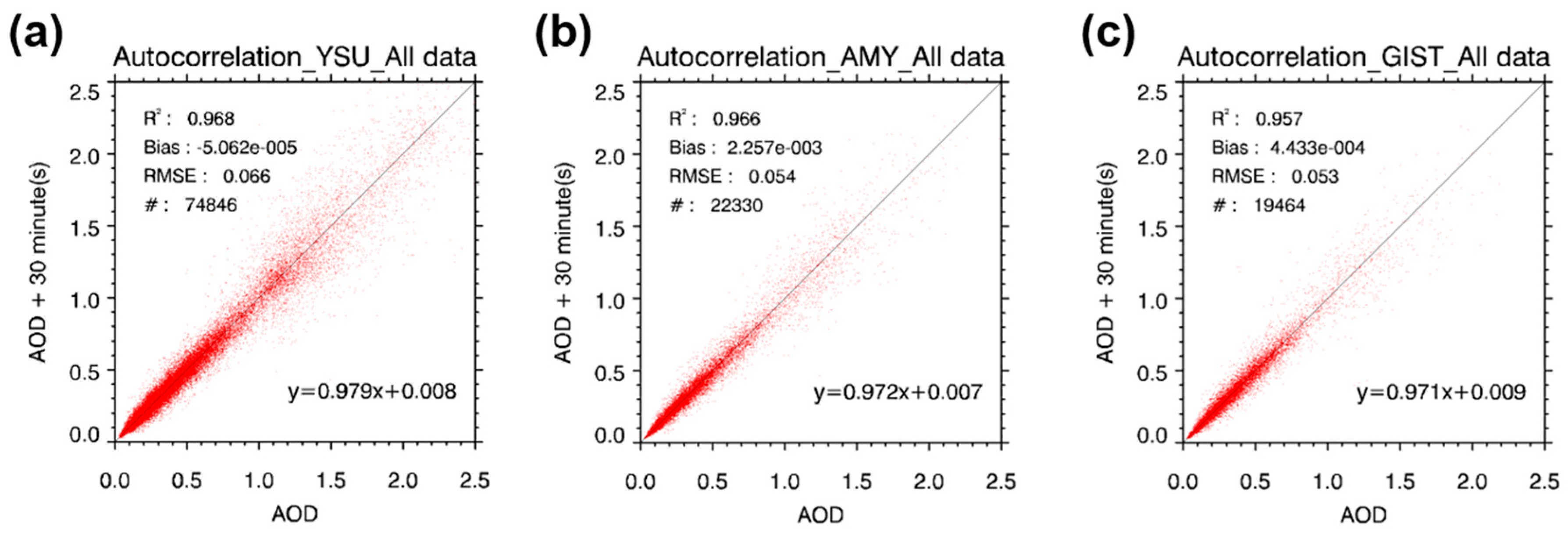
Figure 3 and
Table 2 show the temporal variability of AOD at 500 nm by using data from Sunphotometer in three ground-based stations in Korea. To identify the temporal variability of AOD, the correlation coefficient of determination (R
2), mean bias (MB), and root mean square error (RMSE) were used for the statistical score. In time lags larger than 30 min, the temporal variability of AOD is extremely enhanced, especially for an AOD larger than 1.0. In addition, the RMSE by the temporal variation is significantly larger than the long-term uncertainty of the instrument itself [
62]. As shown in
Table 2, the spread of data increases linearly with the increasing time lag. Because the large AOD cases are caused by the transport of aerosol layers, including dust and anthropogenic pollutants, the spatio-temporal variability of aerosol conditions can change drastically. As the time lag increased, the R
2 values were slightly decreased with increasing absolute values of MB and RMSE (
Table 2). On average, the R
2 difference with 10 min lag increase ranges from −0.0095 to −0.0164, and those differences are more sensitive the larger the time lag is.
The RMSE between the original and time-lagged datasets also increased when the time lag increased. Compared to the expected error range of the satellite algorithm over land, the RMSE that was smaller than the absolute expected error range of satellite algorithm (0.05) only satisfied the case shorter than 20 min of time lag (10 min in YSU). Furthermore, the RMSE difference with 10 min time lag increase is 0.007 to 0.012, and the absolute increasing tendency is largest in YSU. Because the mean value of AOD in Seoul is larger than the other two observation sites, the RMSE in the same time lag is also larger. From the RMSE and R2, the temporal variability is largest in Seoul, and those in the other two observation sites are almost the same. If we assume R2>0.95 and RMSE<0.05 for the same propensity for temporal range, the temporal range of data with the same propensity is 20 min in South Korea.
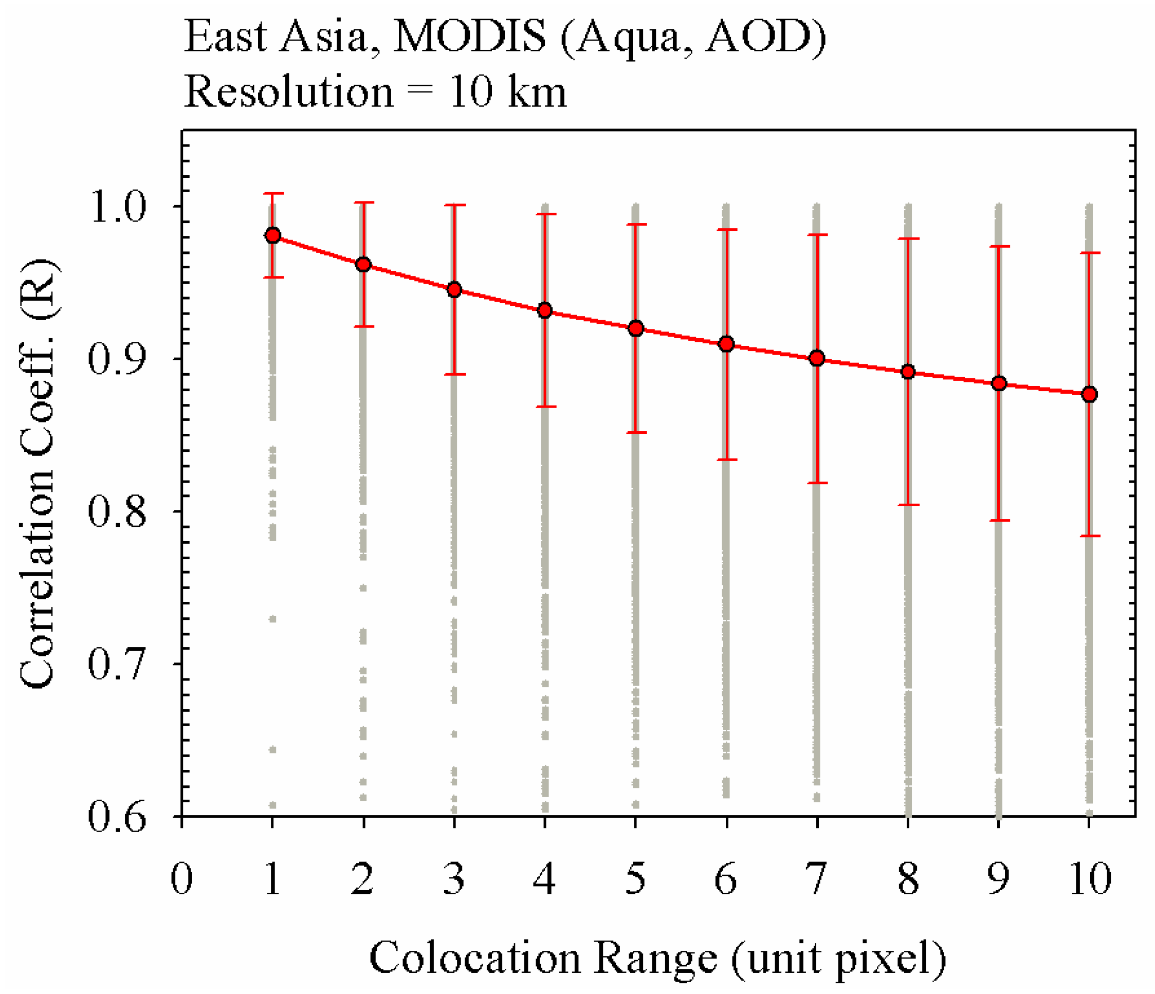
For the spatial variability of AOD from the satellite measurements, the distribution of the correlation coefficient (R
d) was used. For the R
d, each R value was estimated in a single granule in 5-min intervals. Based on each R value, the R
d value was finally calculated to the mean and standard deviation of R values with respect to the colocation range.
Figure 4 shows the R
d value as a function of the colocation range. Focusing on each correlation coefficient value with its respective granule, the R value largely varies by up to ~0.5. The large variation of correlation coefficient in each granule was partially caused by the low AOD values in the background areas, such as the ocean areas. However, statistically estimated mean R
d was higher than the respective R value. The mean R
d ranged from 0.981 in 10 km colocation range to 0.877 in 100 km colocation range. As the colocation range increased, the mean value of R
d slightly decreased as the standard deviation of R
d increased. In addition, as the colocation range increased, the tendency to decrease the mean of R
d and increase the standard deviation of R
d slowed together.
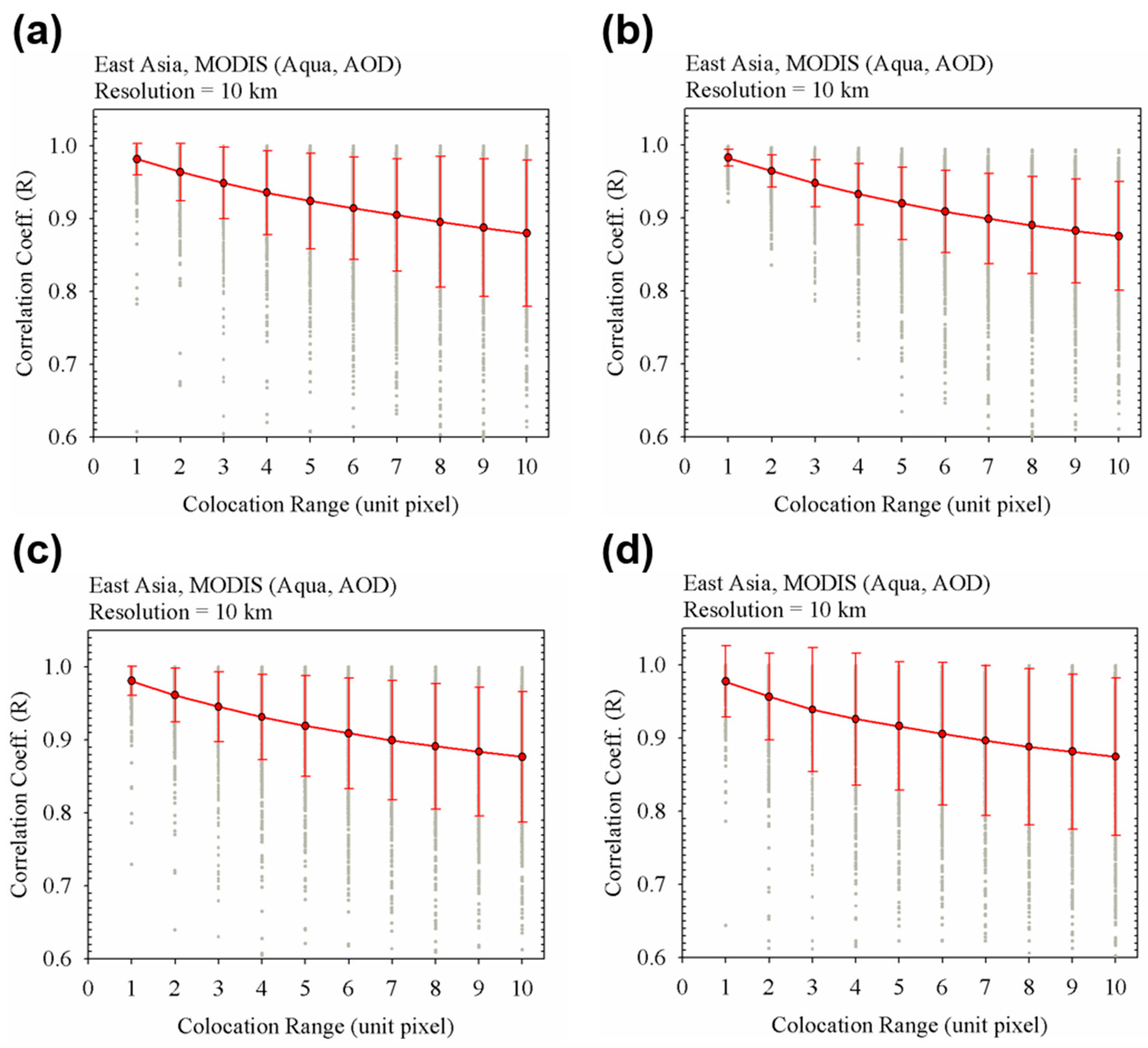
For the seasonal variation, the decreasing tendency of R
d as increasing colocation range has slight seasonal dependency as shown in
Figure 5. While the mean value of R
d has weak seasonal dependence, the standard deviation of R
d is larger in winter and spring than those in summer and autumn. In East Asia, regional transport of aerosol frequently occurs during the late autumn to early spring season through the winter season by the occurrence of dust transport [
63,
64,
65] and haze by anthropogenic emissions [
66,
67]. On the contrary, the trans-boundary transport of aerosol weakens due to decreasing wind speed in the summer and autumn season [
68]. For the seasonal difference of aerosol transport patterns, the regional inhomogeneity of AOD increases in winter and spring, thus, the variation of correlation coefficient with changing colocation range is more sensitive.
4.2. Total Ozone
Table 3 show the temporal variability of TCO in Seoul and Busan. From the statistical analysis, the R
2 and RMSE are 0.966–0.992 and 3.37–7.00 DU in Seoul, and 0.987–0.996 and 2.17–3.98 DU in Busan. In a similar way to the other species, the R
2 has a decreasing tendency and the RMSE has an increasing tendency as the time lag increases. However, the variation of R
2 as a changing time lag is relatively small because the temporal variation of TCO largely depends on the stratospheric ozone variability [
69]. Focusing on the RMSE value, the variability up to 3% of TCO is considerable in the analysis [
38,
70]. In Seoul and Busan, the annual mean value of TCO ranges from 300–340 DU [
44,
71]. For this reason, the temporal variability of TCO is negligible from the Pandora observation.
However, several previous studies have shown that the TCO suddenly changes during winter and spring seasons due to the enhancement of ozone concentration at the upper troposphere/lower stratosphere (UT/LS) in the jet-stream outflow regions [
71,
72,
73]. In East Asia, the UT/LS ozone enhancement frequently occurs, and sudden changes of TCO have frequently been observed based on the daily observation datasets from ground-based measurements [
71]. This phenomenon also affects the spatio-temporal variability of TCO. For this reason, the spatio-temporal variability, considering seasonal change, is also executed to consider the TCO variation due to the UT/LS ozone enhancement.
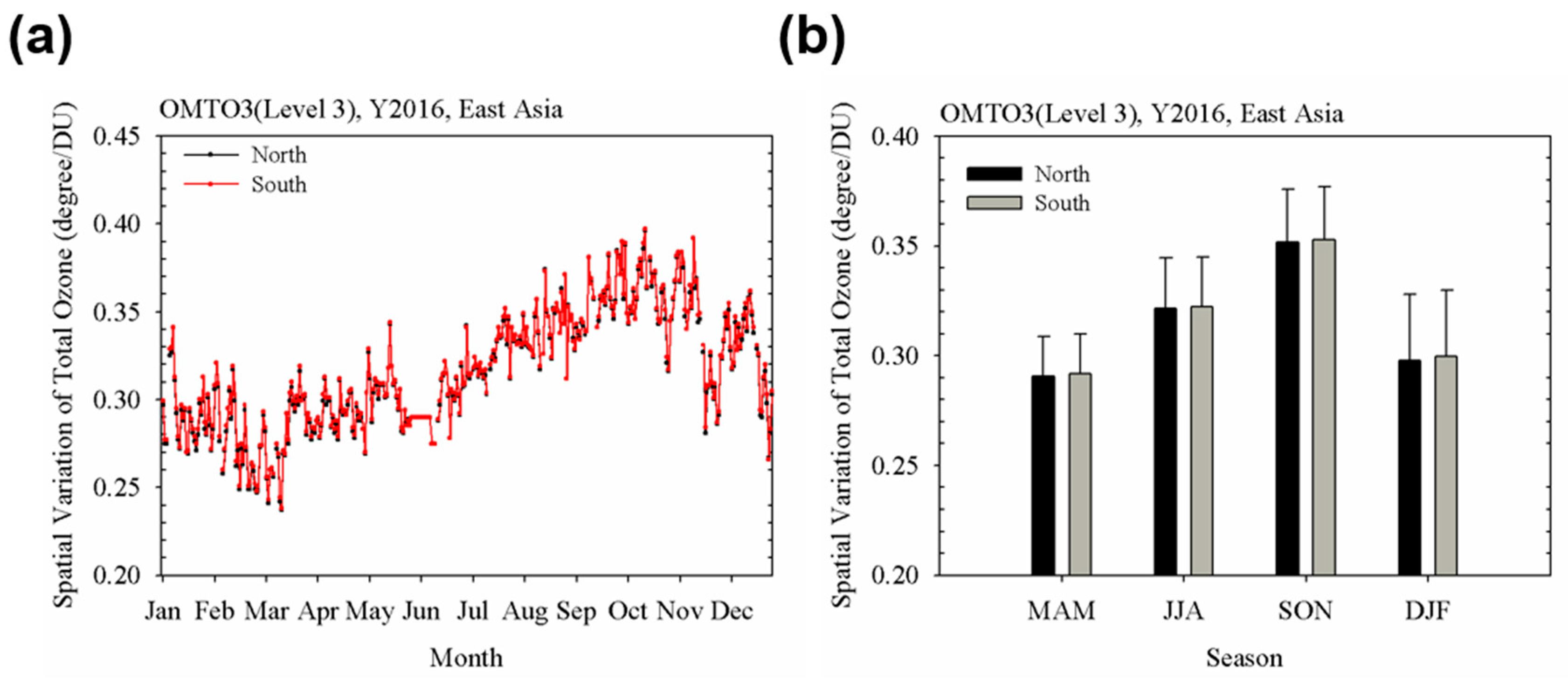
Figure 6 shows the spatial variability of the TCO using Level 3 gridded datasets from OMI in 2016. Because the latitudinal change of TCO is significantly larger than the longitudinal change, the average of the latitude range for 1 DU change was adopted for the estimation of spatial variability of TCO in this study. For the daily statistical results, the spatial variability ranged from 0.237 (12 March) to 0.396 degree/DU (16 October). Categorized by the seasons, as shown in
Figure 6b, the spatial variability is largest in spring (0.29 degree/DU), and smallest in autumn (0.35 degree/DU). Compared to the spring and autumn, there is a 20% difference in the spatial variability. In a similar way to the temporal variability of TCO, large spatial variability in springtime is caused by the sudden increase in the ozone concentration in UT/LS. In addition, the latitudinal gradient of TCO is also related to the Brewer-Dobson circulation, and the intensity of the Brewer-Dobson circulation is strong in wintertime. For this reason, the latitudinal range has to be adjusted according to the season.
4.3. NO2
Table 4 shows the temporal variability for TCN from the Pandora measurements. In a similar way to the AOD analysis, the temporal variability for TCN also used the R
2 and RMSE in their statistical analysis. Over the two ground-based observation sites, the R
2 ranged from 0.880 to 0.565 in Busan and from 0.897 to 0.638 in Seoul. In addition, the RMSE ranged from 0.29 to 0.56 DU, and from 0.15 to 0.31 DU in Seoul and Busan, respectively. Compared to the AOD and TCO results, the R
2 is too low. Because the diurnal variation of the NO
2 was clearly shown in the urban region due to the short lifetime of NO
2 [
51], temporal variability of TCN is larger compared to those of AOD and TCO. The RMSE in Seoul is two times larger than that in Busan. This RMSE difference is caused by the absolute value difference of TCN in Busan and Seoul. From the previous study, the mean value of TCN in Seoul is two times larger than that in Busan during the MAPS-Seoul campaign [
51]. Therefore, the relative value of RMSE to the mean value of TCN is similar in both two observation sites.
As the time lag increases, the decrease of R2 per 10-min time lag shows −0.069 (10 min) to −0.043 (60 min) in Seoul and −0.078 (10 min) to −0.050 (60 min) in Busan. Based on the sensitivity of R2 for time lag, temporal variability is larger in Busan than in Seoul. The large temporal variability in Busan is also identified by the MB and relative value of RMSE. The main reason is the difference in the TCN level in the two regions. Because of the uncertainty from the instrument, the TCN includes the systematic variability during the observation. Without considering the instrument uncertainty, diurnal variation of TCN, due to the emission and photochemical reaction, can also affect the temporal variability in specific points. The temporal variability is similar in the two sites, although the correlation is slightly weaker in Busan than in Seoul. Based on the R2 and RMSE values in the 10-min time lag, if the change in R2 decreased by 0.1 and the RMSE increased by 50%, the temporal range with the data of the same propensity is 30 min in South Korea.
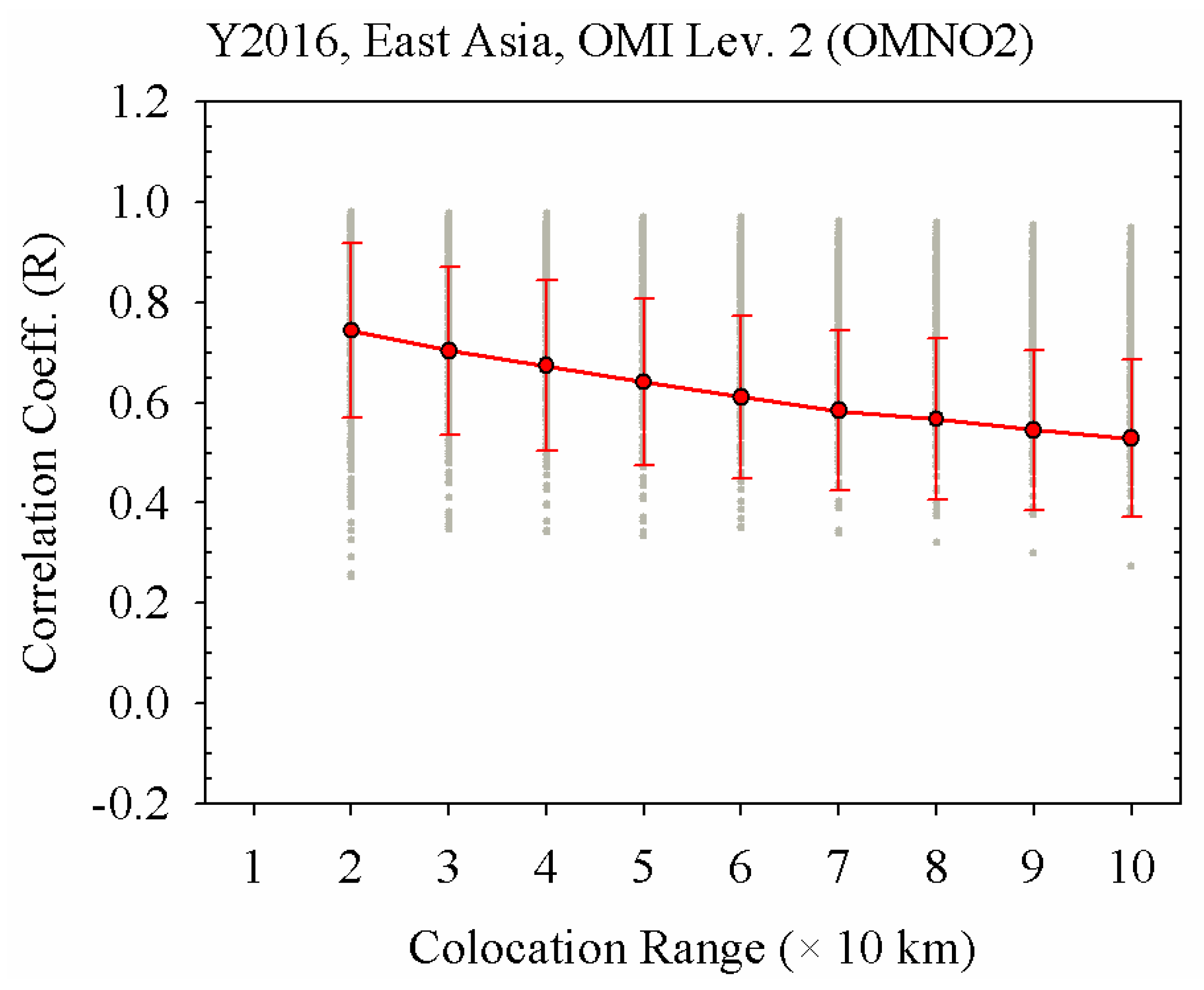
The R
d value for the TCN as a function of colocation range is shown in
Figure 7. Because of the pixel size of OMI, there were no cases within 10 km for the colocation range. In a similar way to the R
d distribution for AOD, a significant tendency to decrease was found with an increasing colocation range. However, the absolute value of R was always smaller than those of the AOD cases. For all cases of the colocation range, the R value did not exceed 0.81. For this reason, it is difficult to apply the threshold of the spatial colocation range for aerosol to those for NO
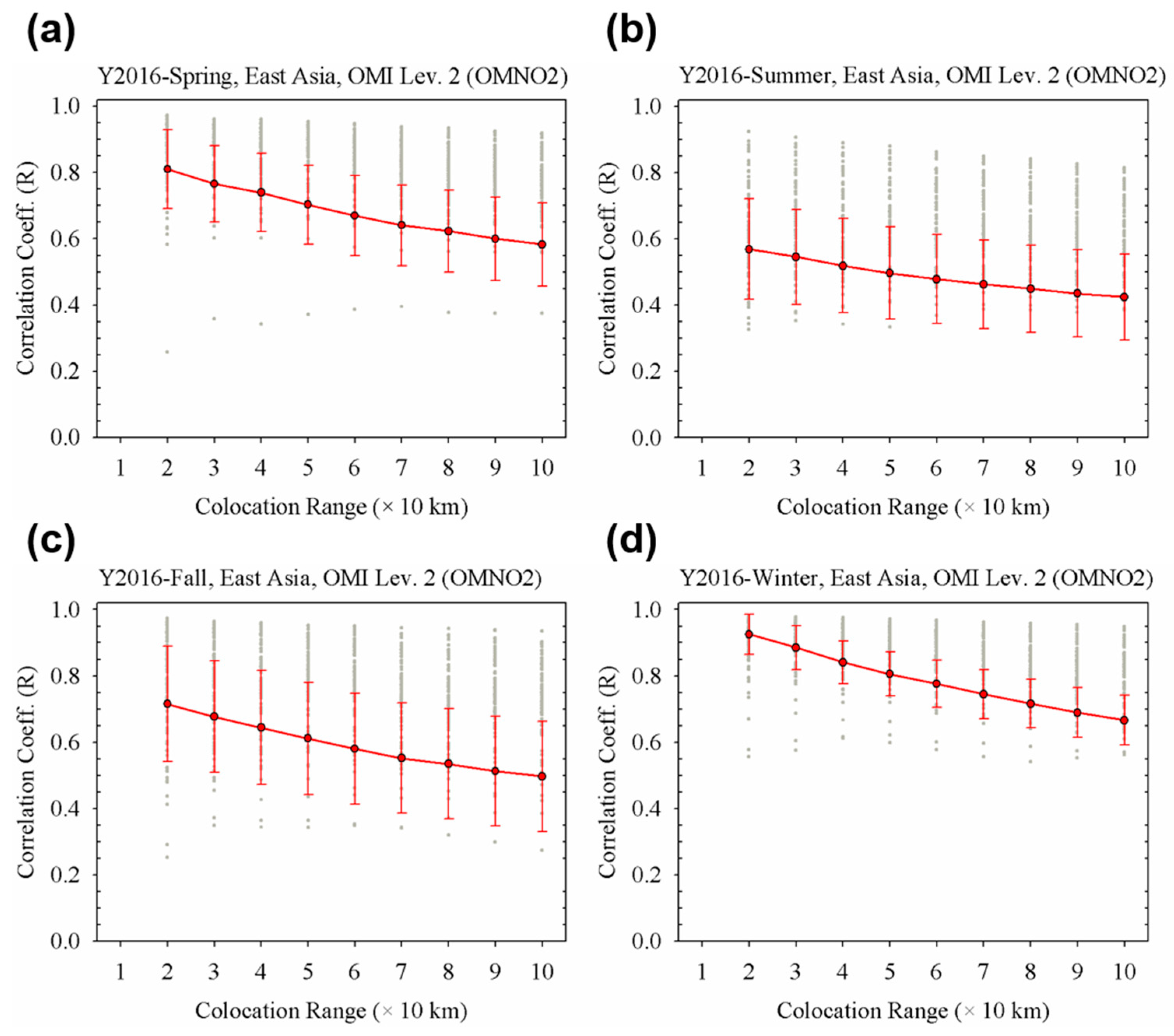
2. Focusing on the seasonal variation, the R
d value has strong seasonal variability, as shown in
Figure 8. Because the photo-chemical reaction vigorously activates in summer [
74], the spatial variability of NO
2 is enhanced during the summer season. In addition, the size of areas in high concentration of NO
2, near the downtown or industrial region, may be reduced due to the photochemical reaction change. For this reason, the R value is up to 0.569 (colocation range: 20 km). Otherwise, the R value is from 0.666 (colocation range: 100 km) to 0.925 (colocation range: 20 km) in wintertime. Therefore, we have to consider the spatial variability of NO
2 because of the strong seasonal variations and inhomogeneity near the emission source regions.
5. Validation Strategy for GEMS Scientific Products
Information of spatio-temporal variability for the amount of species is necessary to identify the temporal and spatial ranges. To determine the spatial and temporal ranges, the datasets observed within the range should be considered statistically as a same quantity. In addition, it is also important to ensure a consistently sufficient amount of data over time and space. Based on the above spatio-temporal variability in
Section 4, we also listed the strategy of the validation for GEMS products in Asia.
Table 5 shows the summary of strategy of the validation plans for the GEMS scientific products, considering spatio-temporal ranges. To determine the spatio-temporal range for the validation, the spatial range is determined by the satellite observation and temporal range is considered by the temporal variation of datasets from ground-based observations. Basically, the validation uses the averaging methods within valid ranges, because the trace gas observations include a large amount of errors during the retrieval process.
For the AOD, the spatio-temporal range for validation is based on R2>0.95 (temporal) and R>0.95 (spatial). From these thresholds, the spatial and temporal validation range is within 30 km and 30 min in all seasons. Especially considering the seasonal variation, the spatial range expands to 40 km in summer and autumn. For the TCO, the temporal variation is negligible due to the time scale of the stratospheric ozone variation. However, the spatial scale is considerable for the latitudinal range. Because of strict target accuracy of TCO, the latitudinal range for TCO is 0.87° in spring to 1.05° in summer, if the threshold of spatial variation of TCO is assumed to be 3 DU. For the TCN, it is difficult to establish rigorous criteria for temporal and spatial agreement. For this reason, the R2 for temporal colocation is assumed to be 0.8. In addition, the rapid increase of RMSE—more than a 50% increase by a 10-min range increase—is also a considerable threshold for temporal colocation. Considering these two criteria, 20 min is suitable for the threshold of temporal range for validation. In the spatial scale, the seasonal considerations are essential. For this reason, the spatial range is 20 km and 50 km for spring and winter, respectively. However, the criteria of R are not satisfied during summer and autumn. In those seasons, the nearest value of satellite data is prioritized for the validation.
6. Summary and Conclusions
As the aerosol and trace gases have large spatial and temporal variabilities due to the complex emission sources and various chemical process, the colocation methods of the dataset are an important consideration factor during intercomparison and validation. From the ground-based and satellite observation datasets, the spatio-temporal variability of AOD, TCO, and TCN were identified over East Asia to define the spatio-temporal range for the GEMS scientific products. Based on the statistical results (R2, RMSE, and MB), optimized spatio-temporal ranges were determined with respect to the target materials. Rd was also used for the satellite observation dataset to define the mean status of the spatial variability of aerosol and trace gases.
For the AOD, the temporal range, as data with the same propensity, was 20 min in South Korea, assuming R2>0.95 and RMSE<0.05 for the temporal scales. From the Rd distribution, the spatial range within 20 km was able to be considered the same value for the validation studies. The Rd distribution also has weak seasonal dependence due to the trans-boundary transport change. For the TCO, the R2 and RMSE was estimated to be from 0.966–0.996 and 2.17–7.00 DU for temporal variation, and 0.237–0.396 degree/DU for spatial variability. The spatio-temporal variability of TCO is affected by the latitudinal gradient change related to the Brewer-Dobson circulation. For the TCN, the R2 and RMSE for temporal variation ranged from 0.565–0.897 and 0.15–0.56 DU, respectively. For all cases of the spatial colocation range, however, the Rd was always smaller than 0.81, which makes it difficult to assume the same value in all spatial ranges. Because of the photochemical reaction change, the spatial variability of TCN has strong seasonal dependence.
Based on the spatio-temporal variability from the observation data, we suggest the basic strategy of the GEMS scientific products. Based on the thresholds of R2>0.95 (temporal) and R>0.95 (spatial), the basic ranges for spatial and temporal scales for AOD validation were found to be within 30 km and 30 min, respectively. In addition, the spatial range was expanded to 40 km in summer and autumn for the consideration of seasonal characteristics. For the TCO validation, the north-south range was the only considerable factor for the validation study due to the seasonal change in the latitudinal gradient. The latitudinal range was set to be from 0.87° in spring to 1.05° in summer. However, the validation criteria for the TCN was difficult because the spatio-temporal variation of TCN was large. Thus, the nearest value in the satellite data was used as the representative data for the validation in summer and autumn. Furthermore, the spatio-temporal range was 20 min and 20–50 km in other seasons.
Although the spatio-temporal variation studies were done using several observation sites, the spatial coverage of ground-based observations had trouble identifying the temporal variability of pollutants. Particularly for formaldehyde (HCHO), it was difficult for the ground-based dataset to observe the total column amount based on the remote sensing instrument. In the future, a geostationary orbit satellite will observe the diurnal variation of atmospheric pollutions, thus the diurnal variation of the spatio-temporal range will be studied.
Author Contributions
Conceptualization, C.-K.S.; formal analysis, S.S.P., J.-U.P. and K.-H.B.; methodology, S.S. Park and C.-K.S.; project administration, S.-W.K. and C.K.S; resources, S.-W.K.; validation, S.S.P. and J.-U.P.; visualization, J.U.P and K.-H.B.; writing—original draft, S.S.P; writing—review & editing, S.-W.K. and C.-K.S. All authors have read and agreed to the published version of the manuscript.
Funding
This research was funded by the Korea Ministry of Environment (MOE) as Public Technology Program based on Environmental Policy (2017000160001), and also supported by the National Strategic Project-Fine Particle of the National Research Foundation of Korea (NRF) funded by the Ministry of Science and ICT (MSIT), the Ministry of Environment (ME), and the Ministry of Health and Welfare (MOHW) (NRF-2017M3D8A1092021).
Acknowledgments
The authors would like to thank the editor and the reviewers’ feedback and suggestions.
Conflicts of Interest
The authors declare no conflicts of interest.
References
- Van Donkelaar, A.; Martin, R.V.; Park, R.J. Estimating ground-level PM2.5 using aerosol optical depth determined from satellite remote sensing. J. Geophys. Res. 2006, 111, D21201. [Google Scholar] [CrossRef]
- Zhang, X.; Kondragunta, S.; Schmidt, C.; Kogan, F. Near real time monitoring of biomass burning particulate emissions (PM2.5) across contiguous United States using multiple satellite instruments. Atmos. Environ. 2008, 42, 6959–6972. [Google Scholar] [CrossRef]
- Duncan, B.N.; Lamsal, L.N.; Thompson, A.M.; Yoshida, Y.; Lu, Z.; Streets, D.G.; Hurwitz, M.M.; Pickering, K.E. A space based, high resolution view of notable changes in urban NOx pollution around the world (2005–2014). J. Geophys. Res. Atmos. 2016, 121, 976–996. [Google Scholar] [CrossRef] [Green Version]
- Curci, G.; Palmer, P.I.; Kurosu, T.P.; Chance, K.; Visconti, G. Estimating European volatile organic compound emissions using satellite observations of formaldehyde from the Ozone Monitoring Instrument. Atmos. Chem. Phys. 2010, 10, 11501–11517. [Google Scholar] [CrossRef] [Green Version]
- Fioletov, V.E.; McLinden, C.A.; Krotkov, N.; Moran, M.D.; Yang, K. Estimation of SO2 emissions using OMI retrievals. Geophys. Res. Lett. 2011, 38, L21811. [Google Scholar] [CrossRef]
- Kim, S.-W.; Heckel, A.; McKeen, S.A.; Frost, G.J.; Hsie, E.-Y.; Trainer, M.K.; Richter, A.; Burrows, J.P.; Peckham, S.E.; Grell, G.A. Satellite-observed U.S. power plant NOx emissions reductions and their impact on air quality. Geophys. Res. Lett. 2006, 33, L22812. [Google Scholar] [CrossRef] [Green Version]
- Turner, A.J.; Jacob, D.J.; Wecht, K.J.; Maasakkers, J.D.; Lundgren, E.; Andrews, A.E.; Biraud, S.C.; Boesch, H.; Bowman, K.W.; Deutscher, N.M.; et al. Estimating global and North American methane emissions with high spatial resolution using GOSAT satellite data. Atmos. Chem. Phys. 2015, 15, 7049–7069. [Google Scholar] [CrossRef] [Green Version]
- Wiedinmyer, C.; Quayle, B.; Geron, C.; Belote, A.; McKenzie, D.; Zhang, X.; O’Neill, S.; Wynne, K.K. Estimating emissions from fires in North America for air quality modeling. Atmos. Environ. 2006, 40, 3419–3432. [Google Scholar] [CrossRef]
- Levelt, P.F.; Van den Oord, G.H.J.; Dobber, M.R.; Malkki, A.; Visser, H.; de Vries, J.; Stammes, P.; Lundell, J.O.V.; Saari, H. The ozone monitoring instrument. IEEE Trans. Geosci. Remote Sens. 2006, 44, 1093–1101. [Google Scholar] [CrossRef]
- Boersma, K.F.; Eskes, H.J.; Veefkind, J.P.; Brinksma, E.J.; van der, A.R.J.; Sneep, M.; van den Oord, G.H.J.; Levelt, P.F.; Stammes, P.; Gleason, J.F.; et al. Near-real time retrieval of tropospheric NO2 from OMI. Atmos. Chem. Phys. 2007, 7, 2103–2118. [Google Scholar] [CrossRef] [Green Version]
- Boersma, K.F.; Eskes, H.J.; Dirksen, R.J.; van der, A.R.J.; Veefkind, J.P.; Stammes, P.; Huijnen, V.; Kleipool, Q.L.; Sneep, M.; Claas, J.; et al. An improved tropospheric NO2 column retrieval algorithm for the Ozone Monitoring Instrument. Atmos. Meas. Tech. 2011, 4, 1905–1928. [Google Scholar] [CrossRef] [Green Version]
- Bucsela, E.J.; Krotkov, N.A.; Celarier, E.A.; Lamsal, L.N.; Swartz, W.H.; Bhartia, P.K.; Boersma, K.F.; Veefkind, J.P.; Gleason, J.F.; Pickering, K.E. A new stratospheric and tropospheric NO2 retrieval algorithm for nadir-viewing satellite instruments: Applications to OMI. Atmos. Meas. Tech. 2013, 6, 2607–2626. [Google Scholar] [CrossRef] [Green Version]
- Lee, C.; Richter, A.; Weber, M.; Burrows, J.P. SO2 retrieval from SCIAMACHY using the Weighting Function DOAS (WFDOAS) technique: Comparison with Standard DOAS retrieval. Atmos. Chem. Phys. 2008, 8, 6137–6145. [Google Scholar] [CrossRef] [Green Version]
- Li, C.; Joiner, J.; Krotkov, N.A.; Bhartia, P.K. A fast and sensitive new satellite SO2 retrieval algorithm based on principal component analysis: Application to the ozone monitroring instrument. Geophys. Res. Lett. 2013, 40, 6314–6318. [Google Scholar] [CrossRef] [Green Version]
- Ahn, C.; Torres, O.; Jethva, H. Assessment of OMI near-UV aerosol optical depth over land. J. Geophys. Res. Atmos. 2014, 119, 2457–2473. [Google Scholar] [CrossRef] [Green Version]
- Torres, O.; Decae, R.; Veefkind, P.; de Leeuw, G. OMI Aerosol Retrieval Algorithm, OMI Algorithm Theoretical Basis Document, Clouds, Aerosols and Surface UV Irradiance; NASA-KNMI ATBD-OMI-03; Harvard Library: Cambridge, MA, USA, 2002; Volume III, pp. 47–71. [Google Scholar]
- Veihelmann, B.; Levelt, P.F.; Stammes, P.; Veefkind, J.P. Simulation study of the aerosol information content in OMI spectral reflectance measurements. Atmos. Chem. Phys. 2007, 7, 3115–3127. [Google Scholar] [CrossRef] [Green Version]
- Griffin, D.; Zhao, X.; McLinden, C.A.; Boersma, F.; Bourassa, A.; Dammer, E.; Degenstein, D.; Eskes, H.; Fehr, L.; Fioletov, V.; et al. High-Resolution Mapping of Nitrogen Dioxide with TROPOMI: First Results and Validation over the Canadian Oil Sands. Geophys. Res. Lett. 2018, 46, 1049–1060. [Google Scholar] [CrossRef] [Green Version]
- Herman, J.; Abuhassan, N.; Kim, J.; Kim, J.; Dubey, M.; Raponi, M.; Tzortziou, M. Underestimation of column NO2 amounts from the OMI satellite compared to diurnally varying ground-based retrievals from multiple PANDORA spectrometer instruments. Atmos. Meas. Tech. 2019, 12, 5593–5612. [Google Scholar] [CrossRef] [Green Version]
- Virtanen, T.H.; Kolmonen, P.; Sogacheva, L.; Rodriguez, E.; Saponaro, G.; de Leeuw, G. Collocation mismatch uncertainties in satellite aerosol retrieval validation. Atmos. Meas. Tech. 2018, 11, 925–938. [Google Scholar] [CrossRef] [Green Version]
- Ichoku, C.; Chu, D.A.; Mattoo, S.; Kaufman, Y.J.; Remer, L.A.; Tanre, D.; Slutsker, I.; Holben, B.N. A spatio-temporal approach for global validation and analysis of MODIS aerosol products. Geophys. Res. Lett. 2002, 29, 1616–1619. [Google Scholar] [CrossRef] [Green Version]
- Cheng, M.M.; Jiang, H.; Guo, Z. Evaluation of long-term tropospheric NO2 columns and the effect of different ecosystem in Yangtze River Delta. Proced. Environ. Sci. 2012, 13, 1045–1056. [Google Scholar] [CrossRef] [Green Version]
- Mishchenko, M.I.; Liu, L.; Geogdzhayev, I.V.; Travis, L.D.; Cairns, B.; Lacis, A.A. Toward unified satellite climatology of aerosol properties. 3. MODIS versus MISR versus AERONET. J. Quant. Spectrosc. Radiat. Transf. 2010, 111, 540–552. [Google Scholar] [CrossRef]
- Su, C.-H.; Ryu, D.; Young, R.I.; Western, A.W.; Wagner, W. Inter-comparison of microwave satellite soil moisture retrievals over the Murrumbidgee Basin, southeast Australia. Remote Sens. Environ. 2013, 134, 1–11. [Google Scholar] [CrossRef]
- De Vries, J.; Voors, R.; Ording, B.; Dingjan, J.; Veefkind, P.; Antje, L.; Kleiipool, Q.; Hoogeveen, R.; Aben, I. TROPOMI on ESA’s Sentinel 5p ready for launch and use. In Proceedings of the 4th International Conference on Remote Sensing and Geoinformation of the Environment (SPIE 9688), Cyprus, Greece, 4–8 April 2016. 96880B. [Google Scholar] [CrossRef]
- Kim, J.; Jeong, U.; Ahn, M.-H.; Kim, J.H.; Park, R.J.; Lee, H.; Song, C.H.; Choi, Y.-S.; Lee, K.-H.; Yoo, J.-M.; et al. New Era of Air Quality Monitoring from Space: Geostationary Environment Monitoring Spectrometer (GEMS). Bull. Am. Meteorol. Soc. 2020, 101, E1–E22. [Google Scholar] [CrossRef] [Green Version]
- Zoogman, P.; Liu, X.; Suleiman, R.M.; Pennington, W.F.; Flittner, D.E.; Al-Saadi, J.A.; Hilton, B.B.; Nicks, D.K.; Newchurch, M.J.; Carr, J.L.; et al. Tropospheric emissions: Monitoring of pollution (TEMPO). J. Quant. Spectrosc. Radiat. Transf. 2017, 186, 17–39. [Google Scholar] [CrossRef]
- Ingmann, P.; Veihelmann, B.; Langen, J.; Lamarre, D.; Stark, H.; Courrèges-Lacoste, G.B. Requirements for the GMES Atmosphere Service and ESA’s implementation concept: Sentinels-4/-5 and -5p. Remote Sens. Environ. 2012, 120, 58–69. [Google Scholar] [CrossRef]
- Goldberg, D.L.; Lamsal, L.N.; Loughner, C.P.; Swartz, W.H.; Lu, Z.; Streets, D.G. A high-resolution and observationally constrained OMI NO2 satellite retrieval. Atmos. Chem. Phys. 2017, 17, 11403–11421. [Google Scholar] [CrossRef] [Green Version]
- Liu, M.; Lin, J.; Boersma, K.F.; Pinardi, G.; Wang, Y.; Chimot, J.; Wagner, T.; Xie, P.; Eskes, H.; Van Roozendael, M.; et al. Improved aerosol correction for OMI tropospheric NO2 retrieval over East Asia: Constraint from CALIOP aerosol vertical profile. Atmos. Meas. Tech. 2019, 12, 1–21. [Google Scholar] [CrossRef] [Green Version]
- Judd, L.M.; Al-Saadi, J.A.; Janz, S.J.; Kowalewski, M.G.; Pierce, R.B.; Szykman, J.J.; Valin, L.C.; Swap, R.; Cede, A.; Mueller, M.; et al. Evaluating the impact of spatial resolution on tropospheric NO2 column comparisons within urban areas using high-resolution airborne data. Atmos. Meas. Tech. 2019, 12, 6091–6111. [Google Scholar] [CrossRef] [Green Version]
- Pan, X.; Uno, I.; Wang, Z.; Nishizawa, T.; Sugimoto, N.; Yamamoto, S.; Kobayashi, H.; Sun, Y.; Fu, P.; Tang, X.; et al. Real-time observational evidence of changing Asian dust morphology with the mixing of heavy anthropogenic pollution. Sci. Rep. 2017, 7, 335. [Google Scholar] [CrossRef] [Green Version]
- Holben, B.N.; Eck, T.F.; Slutsker, I.; Tanre, D.; Buis, J.P.; Setzer, A.; Vermote, E.; Reagan, J.A.; Kaufman, Y.J.; Nakajima, T.; et al. AERONET-A Federated Instrument Network and Data Archive for Aerosol Characterization. Remote Sens. Environ. 1998, 66, 1–16. [Google Scholar] [CrossRef]
- Dubovik, O.; Smirnov, A.; Holben, B.N.; King, M.D.; Kaufman, Y.J.; Eck, T.F.; Slutsker, I. Accuracy assessments of aerosol optical properties retrieved from Aerosol Robotic Network (AERONET) Sun and sky radiance measurements. J. Geophys. Res. Atmos. 2000, 105, 9791–9806. [Google Scholar] [CrossRef] [Green Version]
- Giles, D.M.; Sinyuk, A.; Sorokin, M.G.; Schafer, J.S.; Smirnov, A.; Slutsker, I.; Eck, T.F.; Holben, B.N.; Lewis, J.R.; Campbell, J.R.; et al. Advancements in the Aerosol Robotic Network (AERONET) Version 3 database—Automated near-real-time quality control algorithm with improved cloud screening for Sun photometer aerosol optical depth (AOD) measurements. Atmos. Meas. Tech. 2019, 12, 169–209. [Google Scholar] [CrossRef] [Green Version]
- Buchard, V.; Brogniez, C.; Auriol, F.; Bonnel, B.; Lenoble, J.; Tanskanen, A.; Bojkov, B.; Veefkind, P. Comparison of OMI ozone and UV irradiance data with ground-based measurements at two French sites. Atmos. Chem. Phys. 2008, 8, 4517–4528. [Google Scholar] [CrossRef] [Green Version]
- Bhartia, P.K.; Wellemeyer, C.W. TOMS-V8 Total O3 Algorithm in OMI Algorithm Theoretical Basis Document; Bhartia, P.K., Ed.; NASA Goddard Space Flight Center: Greenbelt, MD, USA, 2002; Volume II, pp. 15–32. [Google Scholar]
- McPeters, R.; Kroon, M.; Labow, G.; Brinksma, E.; Balis, D.; Petropavlovskikh, I.; Veefkind, J.P.; Bhartia, P.K.; Levelt, P.F. Validation of the Aura Ozone Monitoring Instrument total column ozone product. J. Geophys. Res. Atmos. 2008, 113, D15S14. [Google Scholar] [CrossRef] [Green Version]
- Veefkind, J.P.; de Haan, J.F.; Brinksma, E.J.; Kroon, M.; Levelt, P.F. Total Ozone from the Ozone Monitoring Instrument (OMI) using the DOAS technique. IEEE Trans. Geosci. Remote Sens. 2006, 44, 1239–1244. [Google Scholar] [CrossRef]
- Krotkov, N.A.; Lamsal, L.N.; Celarier, E.A.; Swartz, W.H.; Marchenko, S.V.; Bucsela, E.J.; Chan, K.L.; Wenig, M.; Zara, M. The version 3 OMI NO2 standard product. Atmos. Meas. Tech. 2017, 10, 3133–3149. [Google Scholar] [CrossRef] [Green Version]
- De Graaf, M.; Sihler, H.; Tilstra, L.G.; Stammes, P. How big is an OMI pixel? Atmos. Meas. Tech. 2016, 9, 3607–3618. [Google Scholar] [CrossRef] [Green Version]
- Herman, J.; Cede, A.; Spinei, E.; Mount, G.; Tzortziou, M.; Abuhassan, N. NO2 column amounts from groundbased Pandora and MFDOAS spectrometers using the direct-sun DOAS technique: Intercomparisons and application to OMI validation. J. Geophys. Res. 2009, 114, D13307. [Google Scholar] [CrossRef] [Green Version]
- Tzortziou, M.; Herman, J.R.; Cede, A.; Abuhassan, N. High precision, absolute total column ozone measurements from the Pandora spectrometer system: Comparisons with data from a Brewer double monochromator and Aura OMI: Pandora total column ozone retrieval. J. Geophys. Res. Atmos. 2012, 117, D16303. [Google Scholar] [CrossRef] [Green Version]
- Baek, K.; Kim, J.H.; Herman, J.R.; Haffner, D.P.; Kim, J. Validation of Brewer and Pandora measurements using OMI total ozone. Atmos. Environ. 2017, 160, 165–175. [Google Scholar] [CrossRef]
- Kim, J.; Kim, J.; Cho, H.-K.; Herman, J.; Park, S.S.; Lim, H.K.; Kim, J.-H.; Miyagawa, K.; Lee, Y.G. Intercomparison of total column ozone data from the Pandora spectrophotometer with Dobson, Brewer, and OMI measurements over Seoul, Korea. Atmos. Meas. Tech. 2017, 10, 3661–3676. [Google Scholar] [CrossRef] [Green Version]
- Flynn, C.M.; Pickering, K.E.; Crawford, J.H.; Lamsal, L.; Krotkov, N.; Herman, J.; Weinheimer, A.; Chen, G.; Liu, X.; Szykman, J. Relationship between column-density and surface mixing ratio: Statistical analysis of O3 and NO2 data from the July 2011 Maryland DISCOVER-AQ mission. Atmos. Environ. 2014, 92, 429–441. [Google Scholar] [CrossRef] [Green Version]
- Ialongo, I.; Herman, J.; Krotkov, N.; Lamsal, L.; Boersma, K.F.; Hovila, J.; Tamminen, J. Comparison of OMI NO2 observations and their seasonal and weekly cycles with ground-based measurements in Helsinki. Atmos. Meas. Techn. 2016, 9, 5203–5212. [Google Scholar] [CrossRef] [Green Version]
- Lamsal, L.N.; Krotkov, N.A.; Celarier, E.A.; Swartz, W.H.; Pickering, K.E.; Bucsela, E.J.; Gleason, J.F.; Martin, R.V.; Philip, S.; Irie, H. Evaluation of OMI operational standard NO2 column retrievals using in situ and surface-based NO2 observations. Atmos. Chem. Phys. 2014, 14, 11587–11609. [Google Scholar] [CrossRef] [Green Version]
- Lamsal, L.N.; Janz, S.J.; Krotkov, N.A.; Pickering, K.E.; Spurr, R.J.D.; Kowalewski, M.G.; Loughner, C.P.; Crawford, J.H.; Swartz, W.H.; Herman, J.R. High-resolution NO2 observations from the Airborne Compact Atmospheric Mapper: Retrieval and validation. J. Geophys. Res. Atmos. 2017, 122, 1953–1970. [Google Scholar] [CrossRef]
- Nowlan, C.R.; Liu, X.; Leitch, J.W.; Chance, K.; Gonzalez Abad, G.; Liu, C.; Zoogman, P.; Cole, J.; Delker, T.; Good, W.; et al. Nitrogen dioxide observations from the Geostationary Trace gas and Aerosol Sensor Optimization (GeoTASO) airborne instrument: Retrieval algorithm and measurements during DISCOVER-AQ Texas 2013. Atmos. Meas. Techn. 2016, 9, 2647–2668. [Google Scholar] [CrossRef] [Green Version]
- Chong, H.; Lee, H.; Koo, J.-H.; Kim, J.; Jeong, U.; Kim, W.; Kim, S.-W.; Herman, J.R.; Abuhassan, N.K.; Ahn, J.-Y.; et al. Regional Characteristics of NO2 column Densities from Pandora Observations during the MAPS-Seoul Campaign. Aerosol Air Qual. Res. 2018, 18, 2207–2219. [Google Scholar] [CrossRef] [Green Version]
- Tzortziou, M.; Herman, J.R.; Cede, A.; Loughner, C.P.; Abuhassan, N.; Naik, S. Spatial and temporal variability of ozone and nitrogen dioxide over a major urban estuarine ecosystem. J. Atmos. Chem. 2015, 72, 287–309. [Google Scholar] [CrossRef]
- Remer, L.A.; Tanre, D.; Kaufman, Y.J.; Ichoku, C.; Mattoo, S.; Levy, R.; Chu, D.A.; Holben, B.; Dubovik, O.; Smirnov, A.; et al. Validation of MODIS aerosol retrieval over ocean. Geophys. Res. Lett. 2002, 29, 1618. [Google Scholar] [CrossRef] [Green Version]
- Remer, L.; Kaufman, Y.; Tanre, D.; Mattoo, S.; Chu, D.; Martins, J.V.; Li, R.-R.; Ichoku, C.; Levy, R.C.; Kelidman, R.G.; et al. The MODIS aerosol algorithm, products, and validation. J. Atmos. Sci. 2005, 62, 947–973. [Google Scholar] [CrossRef] [Green Version]
- Tanre, D.; Kaufman, Y.J.; Herman, M.; Mattoo, S. Remote sensing of aerosol properties over oceans using the MODIS/EOS spectral radiances. J. Geophys. Res. 1997, 102, 16971–16988. [Google Scholar] [CrossRef]
- Levy, R.C.; Remer, L.A.; Kleidman, R.G.; Mattoo, S.; Ichoku, C.; Kahn, R.; Eck, T.F. Global evaluation of the Collection 5 MODIS dark-target aerosol products over land. Atmos. Chem. Phys. 2010, 10, 10399–10420. [Google Scholar] [CrossRef] [Green Version]
- Hsu, N.C.; Tsay, S.-C.; King, M.D. Deep Blue Retrievals of Asian Aerosol Properties during ACE-Asia. IEEE Trans. Geosci. Remote Sens. 2006, 44, 3180–3195. [Google Scholar] [CrossRef]
- Hsu, N.C.; Jeong, M.-J.; Betternhausen, C.; Sayer, A.M.; Hansell, R.; Seftor, C.S.; Huang, J.; Tsay, S.-C. Enhanced Deep Blue aerosol retrieval algorithm: The second generation. J. Geophys. Res. Atmos. 2013, 118, 9296–9315. [Google Scholar] [CrossRef]
- Steinbrecht, W.; Hassler, B.; Claude, H.; Winkler, P.; Stolarski, R.S. Global distribution of total ozone and lower stratospheric temperature variations. Atmos. Chem. Phys. 2003, 3, 1421–1438. [Google Scholar] [CrossRef] [Green Version]
- Perlwitz, J.; Graf, H.-F. The Statistical Connection between Tropospheric and Stratospheric Circulation of the Northern Hemisphere in Winter. J. Clim. 1995, 8, 2281–2295. [Google Scholar] [CrossRef] [Green Version]
- Salby, M.L.; Callaghan, P.F. Interannual Changes of the Stratospheric Circulation: Relationship to Ozone and Tropospheric Structure. J. Clim. 2002, 15, 3673–3685. [Google Scholar] [CrossRef]
- Kim, S.-W.; Yoon, S.-C.; Dutton, E.G.; Kim, J.; Wehrli, C.; Holben, B.N. Global Surface-Based Sun Photometer Network for Long-Term Observations of Column Aerosol Optical Properties: Intercomparison of Aerosol Optical Depth. Aerosol Sci. Technol. 2008, 42, 1–9. [Google Scholar] [CrossRef]
- Chun, Y.; Boo, K.-O.; Kim, J.; Park, S.-U.; Lee, M. Synopsis, transport, and physical characteristics of Asian dust in Korea. J. Geophys. Res. 2001, 106, 18461–18469. [Google Scholar] [CrossRef] [Green Version]
- Kim, S.-W.; Choi, I.-J.; Yoon, S.C. A multi-year analysis of clear-sky aerosol optical properties and direct radiative forcing at Gosan, Korea (2001–2008). Atmos. Res. 2010, 95, 279–287. [Google Scholar] [CrossRef]
- Kurosaki, Y.; Mikami, Y. Recent frequent dust events and their relation to surface wind in East Asia. Geophys. Res. Lett. 2003, 30, 1736. [Google Scholar] [CrossRef]
- Cheng, X.; Zhao, T.; Gong, S.; Xu, X.; Han, Y.; Yin, Y.; Tang, L.; He, H.; He, J. Implications of East Asian summer and winter monsoons for interannual aerosol variations over central-eastern China. Atmos. Environ. 2016, 129, 218–228. [Google Scholar] [CrossRef]
- Jeong, J.I.; Park, R.J. Winter monsoon variability and its impact on aerosol concentrations in East Asia. Environ. Pollut. 2017, 221, 285–292. [Google Scholar] [CrossRef]
- Kim, S.-W.; Yoon, S.-C.; Kim, J.; Kim, S.-Y. Seasonal and monthly variationso f columnar aerosol optical properties over east Asia determined from multi-year MODIS, LIDAR, and AERONET Sun/sky radiometer measurements. Atmos. Environ. 2007, 41, 1634–1651. [Google Scholar] [CrossRef]
- Fioletov, V.E.; Bodeker, G.E.; Miller, A.J.; McPeters, R.D.; Stolarski, R. Global and zonal total ozone variations estimated from ground-based and satellite measurements: 1964–2000. J. Geophys. Res. 2002, 107, 4647. [Google Scholar] [CrossRef] [Green Version]
- Balis, D.; Kroon, M.; Koukouli, M.E.; Brinksma, E.J.; Labow, G.; Veefkind, J.P.; McPeters, R.D. Validation of Ozone Monitoring Instrument total ozone column measurements using Brewer and Dobson spectrophotometer ground-based observations. J. Geophys. Res. 2007, 112, D24S46. [Google Scholar] [CrossRef] [Green Version]
- Park, S.S.; Kim, J.; Cho, H.K.; Lee, H.; Lee, Y.; Miyagawa, K. Sudden increase in the total ozone density due to secondary ozone peaks and its effect on total ozone trends over Korea. Atmos. Environ. 2012, 47, 226–235. [Google Scholar] [CrossRef]
- Hwang, S.-H.; Kim, J.; Cho, G.-R. Observation of secondary ozone peaks near the tropopause over the Korean peninsula associated with stratosphere-troposphere exchange. J. Geophys. Res. 2007, 112, D16305. [Google Scholar] [CrossRef] [Green Version]
- Lemoine, R. Secondary maxima in ozone profiles. Atmos. Chem.Phys. 2004, 4, 1085–1096. [Google Scholar] [CrossRef] [Green Version]
- Shah, V.; Jacob, D.J.; Li, K.; Silvern, R.F.; Zhai, S.; Liu, M.; Lin, J.; Zhang, Q. Effect of changing NOx lifetime on thhe seasonality and long-term trends of satellite-observed tropospheric NO2 columns over China. Atmos. Chem. Phys. 2020, 20, 1483–1495. [Google Scholar] [CrossRef] [Green Version]
Figure 1.
Monthly variation of number of observation data at (a) Yonsei University (YSU), (b) Anmyeon, and (c) Gwangju Institute of Science and Technology (GIST).
Figure 1.
Monthly variation of number of observation data at (a) Yonsei University (YSU), (b) Anmyeon, and (c) Gwangju Institute of Science and Technology (GIST).
Figure 2.
Pixel selection for spatial variability estimation of aerosol optical depth (AOD) from the moderate resolution imaging spectroradiometer (MODIS).
Figure 2.
Pixel selection for spatial variability estimation of aerosol optical depth (AOD) from the moderate resolution imaging spectroradiometer (MODIS).
Figure 3.
Temporal variability of AOD for 30 min time lag from Sunphotometer at (a) Yonsei University, (b) Anmyeon, and (c) GIST.
Figure 3.
Temporal variability of AOD for 30 min time lag from Sunphotometer at (a) Yonsei University, (b) Anmyeon, and (c) GIST.
Figure 4.
Distribution of correlation coefficient (Rd) for AOD in East Asia with respect to the colocation range.
Figure 4.
Distribution of correlation coefficient (Rd) for AOD in East Asia with respect to the colocation range.
Figure 5.
Distribution of correlation coefficient (Rd) for AOD in East Asia with respect to the colocation range in (a) spring, (b) summer, (c) autumn, and (d) winter.
Figure 5.
Distribution of correlation coefficient (Rd) for AOD in East Asia with respect to the colocation range in (a) spring, (b) summer, (c) autumn, and (d) winter.
Figure 6.
(a) Daily change and (b) seasonal change for latitudinal variability of the TCO by using Level 3 gridded datasets from the Ozone Monitoring Instrument (OMI) in Year 2016.
Figure 6.
(a) Daily change and (b) seasonal change for latitudinal variability of the TCO by using Level 3 gridded datasets from the Ozone Monitoring Instrument (OMI) in Year 2016.
Figure 7.
Distribution of correlation coefficient (Rd) for TCN in East Asia with respect to the colocation range.
Figure 7.
Distribution of correlation coefficient (Rd) for TCN in East Asia with respect to the colocation range.
Figure 8.
Distribution of correlation coefficient (Rd) for TCN in East Asia with respect to the colocation range in (a) spring, (b) summer, (c) autumn, and (d) winter.
Figure 8.
Distribution of correlation coefficient (Rd) for TCN in East Asia with respect to the colocation range in (a) spring, (b) summer, (c) autumn, and (d) winter.
Table 1.
Criteria of Data selection for Pandora.
Table 1.
Criteria of Data selection for Pandora.
| Species | Criteria |
|---|
| Total Ozone | Normalized RMSE < 0.05
SZA < 75 °
Uncertainty < 2 DU |
| NO2 | Normalized RMSE < 0.05
Uncertainty < 0.05 DU
SZA < 70 °
Wavelength shift < 0.01 nm |
Table 2.
Statistical results for temporal variability of AOD with time lag change at (a) Yonsei University, (b) Anmyeon, and (c) GIST.
Table 2.
Statistical results for temporal variability of AOD with time lag change at (a) Yonsei University, (b) Anmyeon, and (c) GIST.
| Time Lag (minute) | R2 | Mean Bias | RMSE |
|---|
| (a) Yonsei University |
| 10 | 0.989 | −0.00007 | 0.037 |
| 20 | 0.978 | −0.00002 | 0.054 |
| 30 | 0.968 | −0.00005 | 0.066 |
| 40 | 0.958 | −0.00026 | 0.074 |
| 50 | 0.947 | −0.00062 | 0.083 |
| 60 | 0.936 | −0.00068 | 0.092 |
| (b) Anmyeon |
| 10 | 0.988 | 0.00010 | 0.032 |
| 20 | 0.977 | 0.00129 | 0.044 |
| 30 | 0.966 | 0.00226 | 0.054 |
| 40 | 0.952 | 0.00267 | 0.063 |
| 50 | 0.940 | 0.00326 | 0.073 |
| 60 | 0.929 | 0.00265 | 0.080 |
| (c) GIST |
| 10 | 0.983 | 0.00038 | 0.032 |
| 20 | 0.973 | 0.00113 | 0.039 |
| 30 | 0.957 | 0.00044 | 0.053 |
| 40 | 0.946 | 0.00232 | 0.056 |
| 50 | 0.927 | 0.00166 | 0.069 |
| 60 | 0.909 | 0.00141 | 0.079 |
Table 3.
Statistical results for temporal variability of total column amount of ozone (TCO) with time lag change in (a) Seoul and (b) Busan.
Table 3.
Statistical results for temporal variability of total column amount of ozone (TCO) with time lag change in (a) Seoul and (b) Busan.
| Time Lag (minute) | R2 | Mean Bias (DU) | RMSE (DU) |
|---|
| (a) Seoul |
| 10 | 0.992 | 0.009 | 3.370 |
| 20 | 0.986 | 0.018 | 4.492 |
| 30 | 0.980 | 0.030 | 5.276 |
| 40 | 0.975 | 0.022 | 5.938 |
| 50 | 0.970 | 0.026 | 6.512 |
| 60 | 0.966 | 0.029 | 6.999 |
| (b) Busan |
| 10 | 0.996 | −0.023 | 2.175 |
| 20 | 0.994 | −0.047 | 2.616 |
| 30 | 0.993 | −0.068 | 2.974 |
| 40 | 0.991 | −0.084 | 3.313 |
| 50 | 0.989 | −0.100 | 3.647 |
| 60 | 0.987 | −0.116 | 3.981 |
Table 4.
Statistical results for temporal variability of total column amount of NO2 (TCN) with time lag change in (a) Seoul and (b) Busan.
Table 4.
Statistical results for temporal variability of total column amount of NO2 (TCN) with time lag change in (a) Seoul and (b) Busan.
| Time Lag (minute) | R2 | Mean Bias (DU) | RMSE (DU) |
|---|
| (a) Seoul |
| 10 | 0.897 | −0.004 | 0.285 |
| 20 | 0.829 | −0.008 | 0.371 |
| 30 | 0.774 | −0.011 | 0.431 |
| 40 | 0.727 | −0.015 | 0.478 |
| 50 | 0.681 | −0.018 | 0.522 |
| 60 | 0.638 | −0.020 | 0.561 |
| (b) Busan |
| 10 | 0.880 | −0.006 | 0.153 |
| 20 | 0.802 | −0.013 | 0.199 |
| 30 | 0.733 | −0.019 | 0.234 |
| 40 | 0.670 | −0.025 | 0.264 |
| 50 | 0.615 | −0.031 | 0.289 |
| 60 | 0.565 | −0.038 | 0.311 |
Table 5.
Strategy of the validation plans for the GEMS scientific products in East Asia.
Table 5.
Strategy of the validation plans for the GEMS scientific products in East Asia.
| Species | Spatial | Temporal |
|---|
| Aerosol | 30 km (Whole Season)
40 km (Summer~Autumn) | 30 min (Whole Season) |
| TCO | 0.87 ° (Spring) ~1.05 ° (Summer) | Negligible for sub-daily scale |
| TCN | 20 km (Spring) ~50 km (Winter) | 20 min |
© 2020 by the authors. Licensee MDPI, Basel, Switzerland. This article is an open access article distributed under the terms and conditions of the Creative Commons Attribution (CC BY) license (http://creativecommons.org/licenses/by/4.0/).


