
Abstract
One major challenge to the improvement of regional climate scenarios for the northern high latitudes is to understand land surface feedbacks associated with vegetation shifts and ecosystem biogeochemical cycling. We employed a customized, Arctic version of the individual-based dynamic vegetation model LPJ-GUESS to simulate the dynamics of upland and wetland ecosystems under a regional climate model–downscaled future climate projection for the Arctic and Subarctic. The simulated vegetation distribution (1961–1990) agreed well with a composite map of actual arctic vegetation. In the future (2051–2080), a poleward advance of the forest–tundra boundary, an expansion of tall shrub tundra, and a dominance shift from deciduous to evergreen boreal conifer forest over northern Eurasia were simulated. Ecosystems continued to sink carbon for the next few decades, although the size of these sinks diminished by the late 21st century. Hot spots of increased CH4 emission were identified in the peatlands near Hudson Bay and western Siberia. In terms of their net impact on regional climate forcing, positive feedbacks associated with the negative effects of tree-line, shrub cover and forest phenology changes on snow-season albedo, as well as the larger sources of CH4, may potentially dominate over negative feedbacks due to increased carbon sequestration and increased latent heat flux.
Export citation and abstract BibTeX RIS

Content from this work may be used under the terms of the Creative Commons Attribution 3.0 licence. Any further distribution of this work must maintain attribution to the author(s) and the title of the work, journal citation and DOI.
1. Introduction
The arctic and subarctic physical environment has recently undergone dramatic changes due to a clear warming trend (Hinzman et al 2005), which was twice or more the rate of the global mean warming (Richter-Menge and Jeffries 2011). Global climate models project an ongoing amplified temperature increase in the Arctic for the next decades (Chapman and Walsh 2007, Koenigk et al 2012). Many studies suggest that environmental variations associated with a warmer climate could have considerable consequences for terrestrial ecosystems, such as changes to their structure, composition and functioning (ACIA 2005). A wealth of observations provide compelling evidence of changes in arctic tundra and boreal forests in response to the recent warming: 'greenness' implied by remotely sensed vegetation proxies (e.g. normalized difference vegetation index, NDVI) over the last three decades mirrors increases in photosynthetic productivity across arctic tundra (Tucker et al 2001, Goetz et al 2007, Epstein et al 2012); transect and plot-scale studies have associated the degree of summer warmth with an increased abundance of shrubs and forbs (Jia et al 2006, Elmendorf et al 2012); repeat landscape photography and dendrochronological analyses have documented northward and upslope shifts of tree-lines during the last century (Kullman 2002, Holtmeier and Broll 2005, Harsch et al 2009, Van et al 2011). Tundra warming experiments and model simulations also indicated that rising temperature could enhance the growth of vegetation by increasing density, statue and abundance of shrubs relative to forbs, graminoids and mosses (Miller and Smith 2012). In spite of the heterogeneity and complexity of the emerging pattern of vegetation change, it is increasingly apparent that arctic and subarctic vegetation is sensitive and undergoing structural and compositional changes in response to ongoing climate change.
Terrestrial ecosystem responses to climate modulate near-surface energy, water and carbon flux between the atmosphere and biosphere. There is concern that arctic warming could be accelerated by the integrated effect of biogeochemical (e.g. carbon exchange) and biogeophysical (e.g. albedo, evapotranspiration) feedbacks associated with vegetation and ecosystem changes, such as those already observed and attributed to recent warming (Serreze et al 2000, Bonan 2008). The carbon-cycle feedback directly influences climate by altering atmospheric carbon dioxide (CO2) concentrations. In the northern high latitudes, a longer and warmer growing season might stimulate carbon uptake through photosynthesis, helping to reduce CO2 concentrations in the atmosphere, and dampening global warming. However, releases of methane (CH4) and CO2 due to enhanced soil decomposition, enhanced thawing of permafrost and increased wildfire could outpace carbon uptake in the future (Friedlingstein et al 2006, McGuire et al 2010, Ahlström et al 2012). The albedo feedback caused by changes in relative extent of vegetation versus exposed snow and ice influences radiative forcing locally and regionally, especially during the late snow season when radiation input is high (Wramneby et al 2010). The current observed shrub expansions, tree-line advances and species shifts could likely decrease local surface albedo, exacerbating regional warming (Shuman et al 2011, Bonfils et al 2012, Miller and Smith 2012). Increased evapotranspiration dampens local warming through increases in latent heat exchange or by increasing the probability of low cloud formation (Wramneby et al 2010, Ban-Weiss et al 2011). Globally, this effect is offset when more heat is transported to the higher atmosphere as water vapor and released during condensation.
Dynamic vegetation models (DVMs) are effective tools for studying the transient impacts of climate change on vegetation structure and composition over wide spatial and temporal scales and to characterize subsequent changes in land surface feedbacks. Previous studies of climate–ecosystem changes over the Arctic have generally employed DVMs with a limited ability to resolve landscape-scale heterogeneity in vegetation composition and structure, employing large-area parameterizations of vegetation dynamics and plant functional types (PFTs) such as 'boreal evergreen tree' and 'cool grass', optimized for global applications rather than the specific nature and dynamics of arctic and subarctic vegetation (for further discussion, see Miller and Smith 2012). Accordingly, we optimized an individual-based dynamic vegetation model LPJ-GUESS (Smith et al 2001) for the application to arctic and subarctic upland and wetland ecosystems. We applied the model under a future climate scenario forced by regional climate model (RCM)-generated fields from the Rossby Center Regional Atmosphere Ocean model (RCAO) (Döscher et al 2002, 2010, Koenigk et al 2011). Compared with the general circulation model (GCM) fields providing boundary conditions to the RCM runs, the RCM-simulated regional climate shows a warmer Arctic, which agrees more closely with ERA-40 reanalysis data in the 20th century. The objectives of this study are to evaluate how well LPJ-GUESS simulates the present-day arctic and subarctic vegetation and to characterize the complex coupling between climate, vegetation and ecosystem changes, as well as the potential feedbacks of such changes to the atmosphere, under the RCAO-generated climate projection, as a case study of potential 21st century climate change over the Arctic.
2. Material and methods
2.1. Individual-based dynamic vegetation model
LPJ-GUESS (Lund-Potsdam-Jena General Ecosystem Simulator; Smith et al 2001) is a dynamic vegetation model optimized for regional and global applications. It shares the mechanistic representation of physiological and biogeochemical processes of the LPJ-DGVM (Sitch et al 2003), but replaces its generalized large-area parameterization of vegetation structure and dynamics with an alternative scheme based on the explicit simulation of woody plant population dynamics, resource competition and stand structure among woody plant individuals and a herbaceous (grass, forb or moss) understory co-occurring within patches differing in age-since-last-disturbance. Replicate patches are simulated to account for stochastic differences in patch development arising from disturbance history, establishment and mortality of simulated woody plant individuals. Individual woody plants are treated as cohorts (age-classes) growing in a number of replicate patches per stand (corresponding to a model grid cell). Population dynamics arise from differential establishment, reproduction, mortality and susceptibility to disturbance among PFTs at the patch scale. PFTs are distinguished by parameters governing their morphology, phenology, shade and drought tolerance, fire resistance and bioclimatic limits. We used 15 PFTs to encompass the major plant types of arctic, subarctic and high-boreal biomes, which comprised boreal and temperate forests, tall and short shrubs, arctic tundra open-ground vegetation (e.g. prostrate dwarf shrubs, graminoid forbs, cushion forbs, lichens and mosses), temperate C3 grassland, wetland graminoids and mosses. The parameterizations of these PFTs were described by Wolf et al (2008), Wania et al (2009b), Miller and Smith (2012), and are given in the supplementary tables S1, S2(a) and (b) (available at stacks.iop.org/ERL/8/034023/mmedia). The version of LPJ-GUESS used in this study has incorporated physical schemes for wetland hydrology, soil water freezing and methane production (Wania et al 2009a, McGuire et al 2012). Methane is produced from a potential carbon pool consumed by methanogens and emerges by one of three pathways: diffusion, plant-mediated transport of dissolved CH4 and ebullition of gaseous CH4 (Wania et al 2010).
2.2. Environmental driving data
The forcing data of LPJ-GUESS comprised daily temperature, precipitation, radiation, wet day frequency, annual atmospheric CO2 concentrations and soil texture-related parameters. Two simulations (the CRU-forced run and the RCAO-forced run) were respectively driven by a 'recent past' climate dataset (CRU TS3.0, 1901–2006) (Mitchell and Jones 2005) and a 'from-recent past-to-future' climate dataset (CRU forcing from 1901 to 1950 followed by 10 years of climate forcing linearly interpolated between CRU and RCAO forcing from 1951 to 1960, and finally RCAO forcing from 1961 to 2080). The RCAO climate was dynamically downscaled from the A1B scenario simulation of the atmosphere–ocean general circulation model ECHAM5/MPI-OM (Koenigk et al 2011). Thus, our simulation domain (e.g. figure 1(a)) is identical to that of RCAO, which extends from about 50° N in the Atlantic sector across the Arctic to the Aleutian Islands in the North Pacific. Annual CO2 concentrations were taken from ice-core measurements and observations for the recent past period (McGuire et al 2001) and from the SRES A1B scenario for the future period.

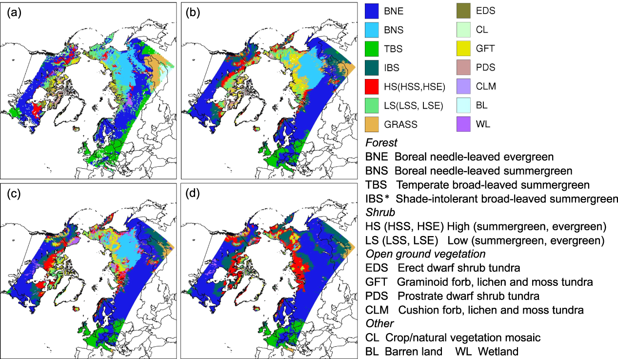
Figure 1. Dominant vegetation distribution. (a) A composite vegetation map based on a potential natural vegetation (PNV) map (Kaplan et al 2003), the IGBP land cover dataset 2000–2001 (Friedl et al 2010), and the Circumpolar Arctic Vegetation Map (Walker et al 2005). (b) The recent dominant PNV simulated by the CRU-forced run. (c) The recent dominant PNV simulated by the RCAO-forced run. (d) The future dominant PNV simulated by the RCAO-forced run. *: the color of IBS represents temperate needle-leaved evergreen forest in the sub-plot (a).
Download figure:
Standard image High-resolution image2.3. Model protocol and evaluation
The model was run twice for each grid cell, once for upland vegetation with 15 replicate patches and once for wetland vegetation using five patches. Replicate patches are simulated to account for the landscape-scale impact of local differences in disturbance history and stand development (see above). The number of patches was chosen to achieve 'stable' results independent of stochastic differences between simulations, while avoiding excessive computing time. Due to the difference between CRU and RCAO coordinates, we used an inverse-distance-weighting algorithm to generate CRU climate for each RCAO grid cell based on climate of the four nearest CRU grid cells. To achieve vegetation, soil carbon and litter pools at equilibrium with the initial forcing climate around 1900, detrended CRU climate data from 1901 to 1930 and 1901s CO2 concentration (296 ppm) repeatedly drove the model for 500 years, switching to recent and the future climate forcing in the subsequent transient phase of the simulations. Relevant model variables (e.g. biomass, carbon pool etc) were aggregated area-weighted by using a prescribed wetland fraction, taken from Kaplan 2007 wetland mapping product (Bergamaschi et al 2007) (supplementary figure S1 available at stacks.iop.org/ERL/8/034023/mmedia).
Vegetation changes were characterized by comparing mean model output for the periods 1961–1990 and 2051–2080 as the recent and the future states. For comparison to the model output, a composite map of observed pan-Arctic vegetation was constructed based on three data sources (supplementary figures S2, S3 and table S3 available at stacks.iop.org/ERL/8/034023/mmedia): a potential natural vegetation (PNV) map (Kaplan et al 2003); the Circumpolar Arctic Vegetation Map (CAVM) (Walker et al 2005); and the International-Geosphere-Biosphere-Program (IGBP) land cover dataset over the period 2000–2001 (Friedl et al 2010). We classified the 15 modeled PFTs based on the biomes types in the observed vegetation map (supplementary table S3). LPJ-GUESS was benchmarked by qualitatively evaluating the recent dominant vegetation distribution in the CRU-forced run. The PFT with the largest biomass within a grid cell was designated as the dominant species. Furthermore, a Kappa analysis (Wolf et al 2008) was employed to measure the goodness-of-fit between the CRU-forced run and the RCAO-forced run. Kappa analysis was carried out in the statistics software IBM SPSS 20.0. We also evaluated the simulated tree-line using the CAVM tree-line boundary dataset. The tree-line was defined as the edge of the habitat where tree species are able to grow, and thus in the model it was treated as the boundary of the grid cells which produced non-zero tree biomass.
2.4. Formulations of the land surface feedbacks
We calculated the changes in net ecosystem exchange of CO2 (NEE) and the net ecosystem–atmosphere CH4 flux. Annual NEE is the balance among net primary production (NPP), soil respiration and carbon released by fire disturbances. Albedo change was quantified according to the method described in Miller and Smith (2012), discriminating summer and winter white-sky albedo for different biomes (supplementary table S1). The proportion of each biome in a grid cell was determined by the total projective foliage cover fraction (FPC) of PFTs included in the biome. FPC is derived from annual leaf area index (LAI) of PFTs according to the Lambert–Beer law (Smith et al 2011). Therefore, the summer or winter albedo in the upland vegetation community (e.g. N biomes, An: the summer or winter albedo of each biome) was calculated from (1), whereas, the wetland biomes' albedo used constant values 0.11 for summer and 0.55 for winter (Moody et al 2007, Houldcroft et al 2009).
The albedo of each grid cell was finally aggregated according to the prescribed wetland fraction. Latent heat feedback was estimated by transforming actual evapotranspiration (ET, mm yr−1) to equivalent latent heat flux E (W m−2) used for water vaporization (Maidman 1992) as (2),

where T is the surface air temperature in degrees Celsius and ρ is the water density in kg m−3. The simulated actual evapotranspiration comprised interception loss, plants' transpiration and bare soil evaporation.
3. Results
3.1. Dominant vegetation distribution and tree-line movement
A qualitative comparison of the dominant vegetation distribution from the CRU-forced run with the observed vegetation map shows a general agreement across most areas of the model domain (figures 1(a), (b)). For example, the simulated conifer forests (BNE, BNS) ring the northern hemisphere, deciduous species (e.g. Larix sibirica) dominating much of northern Siberia; reflecting very low coldest-month temperatures there, with evergreen conifers dominating elsewhere. Forest–shrub–tundra transition zones occur in the Canadian Arctic, northern Alaska, the Taymyr Peninsula of Russia, and the Scandes Mountains. A short vegetation belt along the Chersky mountain range of northeastern Siberia is also clearly reproduced. The major disagreements are exposed in southern Germany where TBS is not simulated as the dominant PFT. In addition, HS dominates some areas classified as LS in the vegetation map. Another mismatch may be explained by the non-inclusion of IBS (e.g. Betula pubescens) on the vegetation map, which nonetheless has been predicted by the model. The composite map also shows a larger area of grassland which is not simulated by either climate forcing, both runs predicting forests rather than grassland. Larger discrepancies between observed and simulated vegetation patterns are revealed in the RCAO-forced run (figure 1(c)). LS are simulated to cover more extensive areas in the Canadian Arctic than PDS and GFT. HS generally expand further north and occupy some lands classified as LS in the vegetation map. Wetland species are simulated to predominate in northern Alaska. A quantitative comparison between the CRU-forced run and the RCAO-forced run by employing Kappa statistics shows the best agreement in the simulated forests, followed by a fair agreement in the simulated shrub-lands and a slight agreement in the simulated open-ground vegetation (supplementary table S4 available at stacks.iop.org/ERL/8/034023/mmedia). In the future climate run, the most noticeable changes are that BNE becomes prominent at the expense of BNS in Siberia (figures 1(c) and (d)). A widespread expansion of HS appears in most areas of the Arctic including the peatlands of Alaska's North Slope. Beringia, Siberia and eastern Canada experience a proliferation of IBS.
The recent tree-line reproduced by the CRU-forced run follows the CAVM tree-line boundary reasonably well, though with a minor overestimation of the northerly forest extent in Vorkuta of western Siberia and an underestimation in the Taymyr Peninsula (figure 2(a)). Trees extend further north in the RCAO-forced run in the Canadian Arctic, but the agreement with the observed tree-line is better in the Taymyr Peninsula. In the future climate run, the tree-line generally shifts north in response to the applied forcing, with the most pronounced shift occurring in the northeast of Siberia (figure 2(b)). Few tree-line recessions occur in Anchorage, Alaska, and on the border between Sweden and Norway.

Figure 2. Tree-line. (a) The simulated tree-line comparisons between the CRU-forced run and the RCAO-forced run. (b) The recent and the future tree-line comparisons in the RCAO-forced run. (Green: the CAVM tree-line boundary; blue: tree-line advance for the latter; red: tree-line retreat for the latter; gray: no difference.)
Download figure:
Standard image High-resolution image3.2. Land surface feedbacks due to vegetation change
We find that the inter-annual variability of NEE is closely associated with the variations of the 2 m air temperature used to force the model (figure 3(a)). Both runs show a slight ecosystem carbon sink in the recent period, though it is slightly larger in the RCAO-forced run. From 1991 to 2006, the annual NEE simulated by both runs lies within the uncertainty range estimated by McGuire et al (2012), who assessed the carbon exchange of arctic tundra by analyzing observations, regional and global process-based terrestrial biosphere models and atmospheric inversion models (table 1). Note, however, that our domain does not exactly coincide with that in McGuire et al (2012). A trend line of annual NEE with a moving average of 6 years indicate that the net carbon sink could continue to increase until 2050 and decline afterwards in spite of continuously rising temperature. From 1901 until 2080, the cumulative net sink of carbon simulated by the RCAO-forced run is 44.72 Gt C, which is comparable to the estimates of 38 ± 20 Gt C for the land north of 60° N by 2100 reported by Qian et al (2010). The most evident spatial changes of NEE in the future are that contemporary forest grid cells tend to experience a reduction in carbon sink whereas grid cells now dominated by shrubs and open-ground vegetation are more likely to experience increased carbon uptake. The largest increase of carbon uptake occurs where conifers are simulated to shift from summergreen to evergreen and in areas of forest expansion on to shrub-lands or tundra (figures 1(d) and 3(b)).
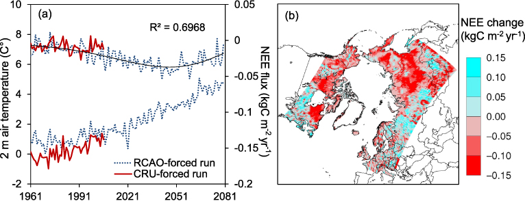
Figure 3. The simulated NEE flux (kg C m−2 yr−1) (uptake: negative; release: positive). (a) The inter-annual variations of the NEE flux (above) and the 2 m air temperature (below) in the CRU-forced run and the RCAO-forced run. (b) The change of the NEE flux between the recent and the future periods in the RCAO-forced run. Note: 1 kg C m−2 corresponds to 17.9 Gt C in this domain.
Download figure:
Standard image High-resolution imageTable 1. The NEE and CH4 flux simulated by the CRU-forced run and the RCAO-forced run (uptake: negative, release: positive). CH4 values are for the wetland fraction of the study area only.
| Period | NEE | CH4 | ||||
|---|---|---|---|---|---|---|
| CRU | RCAO | Referencea | CRU | RCAO | Reference | |
| 1990–1999 (Tg C yr−1) | −242.15 | −247.83 | [−55, −255]b | 46.98 | 67.49 | [15, 34]b |
| 2000–2006 (Tg C yr−1) | −68.78 | −308.23 | [−28, −312]b | 51.64 | 71.68 | [18, 37]b |
| 1901–2080 (Gt C) | — | −44.72 | [−18, −58]c | — | 11.82 | — |
aReference uses the uncertainty range of estimates. bMcGuire et al (2012). cQian et al (2010).
CH4 emissions are simulated to increase over time in all months of the year, with larger increases in the growing season months of June–September (figure 4(a)). Inter-annual variability of CH4 flux tends to be higher in October and May, a result of variation in the onset and length of the active period for growth and microbial activity. Annual CH4 emissions from 1991 to 2006 in both simulations are a little higher than the estimations of McGuire et al (2012) (table 1). One explanation for this may be that our domain includes large wetland areas near Hudson Bay and western Siberia not included in the domain considered by McGuire et al (2012) (supplementary figure S1). By 2080, the total accumulated carbon source due to CH4 emissions is estimated to be 11.82 Gt C. Hotspots of increased CH4 flux emission are found in the Hudson Bay lowlands and in western Siberia, where an additional 20–40 gC-CH4 m−2 yr−1 are simulated in the late 21st century compared to present day (figure 4(b)).

Figure 4. The simulated CH4 flux. (a) The monthly CH4 fluxes from 1961 to 2080. (b) The change of the CH4 flux between the recent and the future periods. Values are for the wetland fraction of the study area only.
Download figure:
Standard image High-resolution imageIn most circumpolar arctic areas, reductions of albedo are simulated both in summer and winter. The resulting change in land surface energy balance may be expected to feed back positively on temperatures, exacerbating climate warming. The winter albedo changes larger as a proportion, though the change is relative to a much lower level of incoming radiation (figures 5(a) and (b)). Spatially, the most pronounced albedo reduction occurs in northern Canada and central Siberia, where substantial vegetation shifts towards increased forest extent and cover are simulated. For example, the expansion of IBS in northern Quebec is simulated to decrease winter albedo by approximately 0.2 and summer albedo approximately 0.04.

Figure 5. The change of the simulated albedo between the recent and the future periods. (a) Summer albedo change. (b) Winter albedo change.
Download figure:
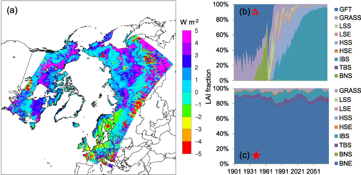
Standard image High-resolution imageThe estimated change of latent heat flux is also consistent with the spatial pattern of vegetation change (figure 6(a)). The largest increase of latent heat flux around 4–5 W m−2 is found in Siberia, Alaska and northern Canada, where either BNE or IBS become dominant species. The rising evapotranspiration could be ascribed to the transition of boreal deciduous forests to shrubs to temperate deciduous forests (figure 6(b)). However, a reduction of the latent heat flux is found in Europe (e.g. Finland, France and Croatia) with a remarkable reduction of 2–5 W m−2. The increased abundance of temperate deciduous forests replacing evergreen trees decreases the total latent heat flux by reducing leaf cover in the early and late active season (figure 6(c)).
Figure 6. The change of simulated latent heat flux associated with modeled species composition in terms of LAI fraction. (a) The change of latent heat flux between the recent and the future periods. (b) Species transition at location (66.46° N, 153.76° E), denoted as the red triangle in (a). (c) Species transition at location (60.87° N, 21.83° E), denoted as the red star in (a).
Download figure:
Standard image High-resolution image
4. Discussion
4.1. Modeling the arctic and subarctic dominant vegetation distribution
Comparing to previous studies in which arctic and subarctic vegetation changes were simulated using either equilibrium biosphere models or global-based DVMs (Kaplan et al 2003, Epstein et al 2007), our simulations differ in highlighting the transient dynamics emerging from the growth and competitive interactions among individual plants co-occurring in local stand, that may be expected when climate is changing rapidly compared with the rate of migration and colonization of species of newly available habitat as the climate warms. Our simulations are capable of capturing major vegetation patterns across the model domain, where climatic gradients are the primary controls of the geographical transition of dominant species from boreal woody plants to short vegetation types. The CRU-forced run explicitly distinguishes graminoid forb tundra, prostrate dwarf shrub tundra and low shrubs according to bioclimatic subzones described by Walker et al (2005). In addition, our simulations incorporate wetland vegetation dynamics, and thus wetland species are shown to be dominating peatland rich areas (e.g. Alaska's North Slope, Hudson Bay and western Siberia) (figure 1(c)).
Uncertainties of PNV modeling are often attributed to factors such as robustness of climate forcing, a lack of detailed soil texture data, topographical factors, nutrient availability, uncertainty in model parameterizations, human interference, and missing physical schemes which are thought to be significant to specific regions or species (Tang et al 2012). These factors among others can account for the discrepancies between simulations and observations. We overestimated boreal conifer forests in some areas of Europe. These places have a long history of human intervention because of agriculture or other land uses. Thus, these areas in the observed vegetation map are unlikely to reflect the actual potential vegetation distribution. Compared to a European PNV map (Hickler et al 2012), the simulated conifer distribution still shows a slight overestimation of range. Soil moisture plays a key role in determining the spatial heterogeneity of arctic tundra vegetation in our model, as prostrate and erect dwarf shrubs cannot survive or compete with graminoid forbs if soil water content is too limited (Kaplan et al 2003). Improved climate forcing and soil property datasets in the high Arctic would potentially improve the accuracy of the predictions for PFTs there. Moreover, the vegetation of the Canadian Arctic as depicted in the CAVM is considered to be affected by an east–west variation in the regional flora due to historical factors such as deglaciation or land bridges, which cannot be accounted for by the model. The under-representation of the grassland vegetation of the central Asian steppe belt in both simulations could be attributed in part to the accuracy of climate forcing. Precipitation is the main factor limiting the establishment of forest in this area in the model. The 'drier' CRU climate produces a larger grassland area in the simulations compared to the RCAO climate (supplementary figures S4(d) and (e) available at stacks.iop.org/ERL/8/034023/mmedia). Compared to the CRU-forced run, the RCAO-forced run shows larger discrepancies in simulating arctic tundra vegetation. This may be traced to the warm regional bias of the RCAO climate forcing centered in the high Arctic (supplementary figures S4(a) and (b) available at stacks.iop.org/ERL/8/034023/mmedia). Higher temperature in the RCAO climate could accelerate the growth of shrubs to become dominant species in terms of their share of total biomass. Although this bias reduces the ability of the model to project the transition between low shrubs and arctic tundra open-ground species in this area, it does not affect the characterization of future tree-line shifts and land surface feedbacks.
4.2. Characterization of future vegetation change
The shifts of TBS and the increased expansions of HS reflect a general northward movement of vegetation transition ecotones, mainly driven by the rising temperatures (figures 1(d), supplementary figure S4). Longer growing seasons and warmer winters advance the spring onset of budburst and photosynthesis, and no longer restrict the northern distributions of temperate species (Woodward 1987, Miller and Smith 2012). The variation of precipitation acted as another important driver for the species which are reliant on soil moisture to adapt to new environments or outcompete other species in the model. In central and northeastern Siberia, the continental climate becomes less pronounced due to the projected warmer winters. The change of climate type could allow BNE or IBS to become predominant at the expense of deciduous needle-leaved species such as larch (BNS). This result is consistent with equilibrium vegetation and forest gap modeling studies (Kaplan et al 2003, Shuman et al 2011). In addition, the study of shrub tundra ecosystems in response to past warming of the Holocene in Beringia based on pollen and macrofossil data indicates a shift from shrub tundra to deciduous forests (Edwards et al 2005). This could also be discerned in the RCAO-forced run (figure 6(b)). The simulated tree-line change projects the movement of the taiga–tundra boundary, the most prominent shift of which was simulated in eastern Siberia, coinciding with an enhanced rate of warming in this area in the RCAO projection (supplementary figure S4). The future tree-line shift in northern Russia is similar to the reconstructed tree-line expansion in the Holocene thermal maximum, but the past tree-line zone was largely occupied by larch due to the low winter and high summer insolation (MacDonald et al 2008).
4.3. Implication for the land surface feedback to climate
The NEE change simulated in the RCAO-forced run suggest that ecosystem could remain as a sink for carbon in a warmer future arctic climate, but the complexity and heterogeneity of compositional and structural responses of vegetation and soils could lead to an overall weakening of the sink, or a shift form a sink to a source of carbon to atmosphere in the long term. Carbon sequestration due to longer growing seasons and CO2 fertilization could be eventually reduced or reversed by increased soil respiration and wildfire disturbances. Shrub-lands continue to act as a weak net carbon sink, but more carbon could be sequestered as new biomass in the stems of trees colonizing new areas rendered suitable for the growth of forest by climate warming. In contrast, contemporary boreal forests could act as carbon sources in future are depleted by accelerated decomposition. A joint consideration of NEE and CH4 in terms of global warming potentials shows that the region is currently a net source of greenhouse gases when expressed in CO2-equivalents (IPCC 2007), and this source is projected to increase 10.4% by 2051–2080, implying that the Arctic may exert a net positive biogeochemical feedback to climate change globally (supplementary table S5 available at stacks.iop.org/ERL/8/034023/mmedia).
Biogeochemical feedbacks associated with carbon balance changes in the Arctic will act globally due to the rapid mixing of the emitted greenhouse gases in the atmosphere. By contrast, our simulations indicate that the biogeophysical feedbacks associated with vegetation adjustments across the Arctic will vary considerably, both seasonally and regionally. In general, displacement of tundra by forest will lead to a local decrease in albedo, which especially in the late snow season, when radiation input is high, will positively feed back to the energy balance of the lower atmosphere, tending to enhance temperature and the rate of climate warming. This positive biogeophysical feedback is likely to be counterbalanced somewhat by the negative local feedbacks due to increased evapotranspiration (Matthes et al 2012). The net effect of both biogeochemical and biogeophysical feedbacks reported here is impossible to quantify exactly in an offline vegetation model, as employed in our study, but is most likely to be positive in this region. This highlights the importance of including dynamic vegetation and biogeochemistry in Earth System Models in order to better assess the impacts of climate change on the high northern latitudes.
Acknowledgments
This study was supported by the project Advanced Simulation of Arctic Climate and Impact on Northern Regions (ADSIMNOR) funded by the Swedish Research Council FORMAS. We thank Rossby Center of Swedish Meteorological and Hydrological Institute for coordinating this project and providing us with regional climate projection data. We thank Jed Oliver Kaplan for providing us with the data of potential natural vegetation map and wetland map. We also thank Dr Annett Wolf for help with model development. This study is a contribution to the strategic research areas Modeling the Regional and Global Earth System (MERGE) and Biodiversity and Ecosystem Services in a Changing Climate (BECC), the Lund University Centre for the Study of Climate and Carbon Cycle (LUCCI) and the Nordic Centre of Excellence DEFROST.