
Abstract
Purpose
The aim of this study is to estimate monetary abatement values for road and rail traffic noise that can be used for policy purposes. However, a main objective is to critically discuss the assumptions necessary to convert the monetary values elicited in willingness to pay (WTP) studies to values than can be use for policy purposes.
Methods
We employ the hedonic regression technique on Swedish data to elicit individuals’ preferences for noise abatement. Our elicited values are then converted to policy values and critically examined based on findings from a literature review.
Results
We show that WTP for road and rail not only differs in levels but also that the relationship between the noise level and the marginal value differs between the two sources. We also show that a health cost component added to the WTP estimate, based on the assumption of uninformed property buyers, will be small but not negligible and that also modest differences in the assumption of the discount rates will have a significant effect on the estimated values.
Conclusions
The main implications from this study are: (i) WTP for road and railway noise abatement differs not only on absolute but also marginal levels, (ii) Even small differences in the chosen discount rate, which is necessary to convert WTP values from a hedonic price study to policy values, have large effects on the policy values, and (iii) We show how to add a health cost component to the WTP estimates in order for the monetary estimates to reflect the total social cost. However, we argue that the motivation for doing so is weak and that more research is needed on this issue.
1 Introduction
Noise is a considerable social problem. For example, more than 20 % of the EU’s population are exposed to higher levels of noise than are deemed acceptable [22]. Prolonged exposure of noise is also a health problem, the World Health Organization (WHO) estimates that more than 1 million healthy life years are lost every year in western Europe due to noise exposure [7]. The transport sector is a principal contributor to society’s noise problem, and the combination of increasing traffic volumes and urbanization means that the problem will increase if no measures are taken to curb it [14, 15, 34, 49]. Road traffic is the largest single source of noise in the transport sector, but other modes such as aircraft and trains also contribute substantially to the noise emissions [33, 39, 67].
The negative effects of the noise may be reduced through legislation, e.g. requirement of less noisy technology, investments, such as noise barriers, or infrastructure use charges that punish more noisy vehicles and lead to a reduction of the noise level. Noise-reducing measures often come at a cost, however, for instance longer traveling times or costs of physical measures such as noise barriers and façade insulation [20, 53]. This, and the fact that society also faces other needs, implies that there has to be some form of prioritization when it comes to resource allocation. Benefit-cost analysis (BCA) is a potential basis for decision making, but it requires, though, both benefits and costs to be measured in a common metric.
Monetary values act as this common metric and in this paper we estimate monetary values for road- and rail-traffic noise abatement. These two noise sources are of different character and it is well established that the annoyance from noise individuals report differs between the two modes of transport [41]. The origin of this paper was a recent revision of the official monetary benefit measures of noise abatement, from now on the “ASEK values”,Footnote 1 carried out in Sweden [65]. The original values were revised to take into account general price increases and an increase in real growth. It was also decided that the original values should be adjusted upwards since it was assumed they they did not reflect the total social cost, but were missing the social cost of health effects from noise exposure [65]. This revision drew to the attention the potential need for a more comprehensive revision due to the fact that the values for all transport modes were based (after also other sources had been taken into consideration) on estimates from a study in which the effect on property prices from road noise was examined [63, 71].
Thus, the aim of this study is to estimate monetary abatement values for road and rail traffic noise that can be used for policy purposes. The main objective is twofold: (i) to estimate monetary values that can be used for BCA in Sweden, and (ii) to examine the magnitude of the difference in estimates between road and railway noise. The former is mainly of policy relevance; both for BCA in which today often the social cost of noise is ignored [19, 47] and for the pricing of the noise externality in transportation based on the social marginal cost principle [2, 3]. The latter objective has both a policy and research relevance. Benefit measures are usually not elicited for all noise sources and by examining to what extent they differ we test to what extent values for one noise source can be used as a measure for the other source, i.e. a test of the use of benefits transfer [58]. Moreover, two additional objectives is to address the question whether derived benefit measures need to be augmented by a health component and to examine the sensitivity of the estimates as a result of assumptions on discount rates. The issue about the health component refers to whether individuals are informed about negative health effects and their costs when they reveal their willingness to pay (WTP) to reduce their noise exposure. If not, this needs to be taken into account when calculating the benefit measures. To estimate the social value of noise abatement we combine measures reflecting individuals’ preferences for reducing noise levels from a Swedish hedonic property price study [1] with estimates for the social cost related to health effects from noise exposure.
This paper is structured as follows. The next section briefly discusses the characteristics of noise, depending on the transport mode, and how this affects the individual’s annoyance level, assumptions about the social cost of noise exposure, various methods of estimating the social costs, and a review of evaluation studies. We thereafter in Section 3 describe and show results of the evaluation of the social cost of noise in this study, i.e. the WTP estimates used and the evaluation of health effects. Section 4 then contains our models on how to combine the different cost components and our estimated benefit measures. In this section we show that the values for road and rail not only differ in levels but also that the relationship between the noise level and the marginal value differ between the two sources. The social value for railway noise reveals a stronger progressive relationship with the noise level compared with road noise. Moreover, we also show that the health cost component added to the WTP estimate will be small but not negligible and that also modest differences in the assumption of the discount rates will have a significant effect on the estimated values. The paper ends with a discussion and conclusions.
2 Noise—characteristics, social costs and evaluation
In the first part of this section we briefly describe how noise is measured and evidence on how individuals are annoyed by different types of traffic noise. We then describe the different social noise cost components, and end this section with a summary of previous findings in the literature.
2.1 Acoustics and annoyance
The A-weighted sound pressure level, measured over 24-h and usually denoted  , is often used as an indicator of noise levels. It is an energy mean level and correlates well with the general annoyance due to noise at a given place. A more relevant measure for sleep disturbance is the maximum level combined with the number of occurrences (
 ).
).
Different sources have different noise profiles over a 24-h period. Rail traffic sometimes has a higher proportion of freight trains running at night, and it is therefore not unusual for the equivalent level at night (23–07) to be higher than during the day (07–19). Road traffic reaches its peaks in the morning and afternoon, but there may sometimes be heavy traffic at night. Air traffic resembles road traffic in its distribution but with fewer and noisier events per 24-h.
Noise sources also differ when seen in a shorter time perspective (variations over minutes). Both rail and air traffic typically have a high maximum level compared to the equivalent level; that is, the individual passages are separated, with silent periods in between. Road traffic tends to have a more even level: that is, smaller differences between maximum and equivalent levels. Note, though, that there are exceptions; for example, low-traffic roads with a high proportion of heavy vehicles may be more like railways in terms of the noise profile.
The EU joint noise indicator  is an attempt to balance the 24-h effects of traffic. This is, in principle, a weighted equivalent level where passages in the evening and at night are counted as 5 dB and 10 dB noisier, respectively, than is actually the case. Thus, evening and night time noise are “punished” in the sense that they are given more weight in the model. This is also applicable to air traffic.
The evaluation of annoyance due to traffic noise by means of questionnaires is often carried out on a 5-point scale, in accordance with ISO/TS 15666 [30]. One can also predict the number of people on the various annoyance levels according to [23], which is based on a metanalysis of many studies [41]. Note that the noise indicator used is  , which is why one must know the traffic distribution over a 24-h period to be able to apply the prediction when only the equivalent level
  is known. Miedema and Oudshoorn [41] clearly shows that the proportion of people who are annoyed at the same noise level (
 ) is largest for air traffic and lowest for rail traffic, with road traffic in between.
2.2 Social costs of noise exposure
Noise does not cause any direct environmental damage but incurs costs for society in the form of disturbances for the individual (sleep, conversation, recreation, etc.), worsened health and loss of production. The latter may be due to absence from work or reduced capacity to work, or that not getting a good night’s sleep means that the individual is less productive than usual. The social costs of noise exposure may be divided into three groups (e.g. [2]):
-
1.
Resource costs in the form of medical and health care. Includes costs financed by taxes and direct payments by the individual.
-
2.
Opportunity costs in the form of loss of production. Includes “non-market services” carried out in the household and lost recreation time.
-
3.
Dis-utility in the form of other negative influences resulting from noise exposure. Disturbances in different forms and increased concern about the after effects as a result of exposure are two examples.
Since the three components are not completely separable, an adding up of the three would mean an overestimation of the social cost. While the first two components, Resource costs and Opportunity costs, the sum of which is usually termed “Cost of illness” (COI) in health economics literature, may be estimated with existing market prices, there are no directly observable market prices for Dis-utility. Dis-utility is therefore estimated by means of the WTP approach, an approach that is usually divided into two main groups depending on what information is used. Preference estimates based on market data and hypothetical market situations are called “revealed preferences” (RP) and “stated preferences” (SP), where the notations show whether the actual or hypothetical choice is used. If individuals in the WTP studies were fully informed of the total cost of noise exposure and if they themselves bore the costs completely, the values from such studies would reflect the social costs in the form of COI as well. It has been suggested based on the assumption that individuals are not fully informed of the negative effects of noise that WTP values should be augmented with a health cost component (e.g. [12, 42]).Footnote 2 Whether this is indeed the case has not been proven, though. Hence, the evidence of the necessity of augmenting the WTP values with a health cost component is weak.
2.3 Overview of WTP studies
An overwhelming majority of the WTP studies to elicit preferences for noise abatement have employed the RP-approach using the hedonic price regression technique [47]. By studying how property prices are affected by noise exposure, at the same time as controlling for the effects from other attributes on the prices, house owners’ preferences for noise abatement can be elicited. The “noise sensitivity depreciation index” (NSDI) has evolved as the standard measure of the WTP of this literature. This is a measure of the percentage change in the price as a result of a unit change in the noise level [45]. Footnote 3 The strength of HP studies lies in the fact that they are based on individuals’ actual choices. A shortcoming is that it can be difficult, and sometimes impossible, to estimate the values of interest, for example the WTP for noise reduction at different times of the day [17]. The methods that use the SP approach offer flexibility, but the hypothetical scenario is their weakness.Footnote 4 The SP method most often used to evaluate noise is the “contingent valuation method” (CVM) [43], in which the respondents directly state their WTP for the good, here a reduction of the noise level. The strength of the CVM and other SP methods, as mentioned above, is that the analyst him/herself constructs the study and may therefore ask questions he/she wants answers to and control for how various factors, such as study design, may have affected the results.
We start this overview of evaluation studies on noise abatement by focusing on Swedish studies. Table 1 contains Swedish WTP studies for traffic noise. As shown in the table, two studies use the hedonic approach and thereby market data [28, 71], while four studies use a hypothetical approach, either CVM [12, 35, 70] or “stated choice modelling” (SCM) [17]. The two hedonic studies employ the effects of traffic noise on property prices in Täby [28] and Ängby [71], both outside Stockholm, and estimated only the effect of road noise. Both studies found that the estimated percentage depreciation was progressively increasing with the noise level.
The EU project HEATCO [12], carried out in several European countries, was aimed at estimating the WTP to reduce noise from road and railway traffic.Footnote 5 Only individuals’ WTP for a reduction of road traffic noise was estimated for Sweden. The results of the studies revealed a methodological problem. For example, the proportion that accepted the payment of a certain amount did not decrease monotonically with the level of the offer, and a large proportion stated they were not willing to pay although they admitted that they were disturbed, while others had a positive WTP even though they were not disturbed. As a consequence, the validity of the estimations is open to question. Bickel et al. [12] chose not to use the new results, but to base the recommended calculation values on the results from [42] in which an ”EU-value” was calculated [11]. The values in [12] show a weak progressive relation, two segments with constant marginal costs.
Turning to the international literature, we find that most WTP studies have concentrated only on one noise source, usually the effect from air- or road-traffic noise on property values. In their overview of existing studies [8] and [42] report NSDI values for road traffic in the interval 0.08–2.22 % and 0.08–2.3 %. Bateman et al. [8] also find an average of ca 0.55 for the studies; that is, this mean value implies that a 1 dB increase leads to a reduction of property values by a little over half a percent. Nelson [46] analyzed 20 hedonic studies on air traffic noise in the USA and Canada in a meta analysis with NSDI in the interval 0.28–1.49 and an average of 0.6. In a new review by [47] interquartile means of 0.80 % and 0.51 % for air and road traffic noise were reported.
Two studies evaluate air, road and rail traffic noise [19, 21]. The principal interest in [21] is the evaluation of air traffic noise, but the analysis is extended to include road and rail traffic noise as well. Various threshold levels are used for the different noise sources; it is assumed that the level at which noise is not annoying varies, depending on whether the noise comes from air or road or rail traffic. For aircraft traffic the limit is set to 45 dB while road traffic is considered annoying at a level over 55 dB and rail traffic over 60 dB. Dekkers and van der Straaten [21] maintain that the choice of threshold level affects the results of the model and advocates caution when interpreting and using their results in which NSDI for air traffic is estimated at 0.77, while rail traffic has NSDI of 0.67 and road traffic 0.16. Day et al. [19] is based on estimates from 8 sub-markets, which give NSDI from 0.18 % to 0.55 % for road traffic noise while the models for rail traffic noise indicate a higher NSDI around 0.67 %. For air traffic noise the results are “erratic”, which, according to [19] is explained by the very few properties subjected to air traffic noise in the data set. Day et al. [19] also estimate the theoretically consistent welfare measures for non-marginal changes, the second step in the hedonic method [61].Footnote 6
Examples of other recent SP studies (besides HEATCO) on the evaluation of traffic noise are [5, 13, 26, 27, 52], and [37].Footnote 7 To summarize, there is considerable variation in the results in the SP studies, and not always in the direction one expects based on the wealth level of the countries. However, for brevity, since our empirical application is a Swedish RP study, we do not discuss these SP studies in detail.
3 Estimation of the cost components
We start this section by describing the evaluation technique used to derive monetary values for noise annoyance and the empirical study that was conducted. In the second part we describe the estimation of the health cost component.
3.1 Evaluation of annoyance
3.1.1 Hedonic regression
Individuals’ WTP for a reduction of their noise exposure is estimated using the hedonic regression method [61].Footnote 8 The estimates are based on price data from the property market and, according to the hedonic method, the price (P) is assumed to be a function of the various attributes that constitute the property,

where  and
and  denote the noise attributes road (
 ) and railway (
 ) and a vector with other attributes. By studying how the price varies depending on the different levels of the attribute of interest, at the same time as controlling for the effects of other attributes, the individuals’ marginal WTP can be estimated. Let
  , denote the marginal WTP for a reduction of the noise level from source i, which is given by,

Equation 2 gives the marginal WTP. To estimate the theoretically consistent welfare measure for non-marginal changes, the demand functions should be estimated. This is often referred to as the second stage of the hedonic method and was carried out in [19]. An alternative, which assumes that the hedonic price function does not change as a result of the change in noise levels, is to base the individual’s welfare change on the price function. The individual’s welfare change is then given by the price change and even if it is not theoretically consistent it is a good measure of WTP for small changes in noise levels. This evaluation approach is based on an assumption of zero moving costs, making the value an upper limit for the individual’s WTP.Footnote 9 In this study we only conduct the first step and, therefore, estimate the monetary values using the hedonic price function.
3.1.2 Econometric analysis
The estimated WTP used in this paper is based on [1]. Since the data were also analyzed in [1] we only provide a terse description of the study and the results that are of interest to our analysis in this article.Footnote 10 To conduct their empirical analysis Andersson et al. used a pooled data set for Lerum, a municipality close to Gothenburg, which consisted of two sources; property noise levels from a study on the health effects of traffic noise conducted in Lerum in 2004 [56] and property prices and other attributes (besides the noise variables) from the National Land Survey of Sweden. Descriptive statistics for the different variables are listed and described in Table 5 in the Appendix. Prices are reported in 2004 price levels and the explanatory variables used in the regression are Living space, Quality index, Terraced, Linked and Detached which describe property attributes, whereas the other variables, besides the two noise variables, describe geographical attributes of the properties. Of the latter variables one is a dummy for distance to the motorway, E20 150m, a proxy for other negative effects from living close to the road besides road noise, two are measures of the distance to nearest train station and motorway entrance, Dist. station and Dist. entrance, i.e. measures of positive effects of the railway and motorway, whereas the other geographical variables define different neighborhoods.
The two variables defining the noise indicators are our variables of main interest. These two variables reflect the equivalent noise levels  and were calculated by [56] using the “Nordic methods” [32, 48]. Since they calculated the noise levels for both rail and road noise for each property we have access to unusually rich data on noise levels. The noise variables are in the regressions defined by the absolute noise level minus 45, with 0 for levels below 45 dB. The effect from noise on the property price should be zero when no negative effect is observed, and in our study we have chosen to use a lower limit of
  dB. The limit is somewhat arbitrarily determined, but the percentage of persons reporting that they are annoyed by traffic noise is very low below this level [41].
When choosing the functional form of the hedonic price function economic theory leaves us without much guidance [61]. Different forms were tested in [1] and based on their results, which revealed the necessity of allowing for a flexible price function, and expectations based on evidence from the acoustical literature, our preferred hedonic price function has the following form,

where

The noise variables are given by  (set to zero for negative values, i.e. if noise levels are below 45 dB) with subscript i and j denoting single properties and road (1) and rail (2), respectively. Other property attributes besides the noise variables are given by
  , and
, and  , b, and k are the parameters to be estimated. In Eq. 4 the parameter b corresponds to the maximum effect at the highest noise level 75 dB in the study area and k describes the concavity of the function. In the regression, the parameter k is restricted to be between 0 and 1 and is estimated as,

thus c is the parameter that is estimated in the regression. Note that b and k are estimated separately for road and rail noise. Hence, Eq. 3 makes it possible to assume not only different maximum effects from road and rail noise, but also different degrees of concavity for the two noise sources. Moreover, to get a more homogeneous sample only properties with a total noise level of at least 50 dB, i.e. the official Swedish threshold value for when noise is assumed to be disturbing, were included.Footnote 11
The regression results and the NSDI estimates based on these results are shown in Table 2.Footnote 12 The hedonic regression is based on non-linear estimation and we first focus on the variables not defining noise levels. We find that the property attributes are all statistically significant and with the expected signs. Regarding the neighborhood dummies we find that some are significant compared to the reference group (Floda 2). Moreover, we find no evidence that the prices of properties situated within 150 m from the motorway E20 are significantly affected by the motorway, given that the noise level is controlled for. Further, Dist. station and Dist. entrance are both not statistically significant. The coefficients for the noise variables are our main interest. The relevant hypothesis testing regarding the noise variables is to test whether the b coefficient is equal to one, since  suggests that the price is not influenced by the noise level. We find that the coefficient for road noise is statistically significant different from one, but not for railway noise. For the k-parameter, calculated using the coefficient estimate of
  (see Eq. 5), a higher value implies a more concave function and a value close to zero implies an almost linear relationship between the noise level and the property price. The results, therefore, suggest a more concave relationship for rail than road noise.
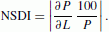
The last two columns of Table 2 show NSDI values for 4 different noise levels. The NSDI is given by

which, since other attributes cancel, only depends on the noise level.Footnote 13 The NSDI increases with the noise level and the higher degree of concavity for rail noise leads to lower NSDI values from rail noise than road noise for low noise levels but higher values for very high noise levels. The effect of rail noise on the property prices is lower than the effect of road noise for all noise levels except the highest (70 dB).
3.2 Evaluation of health effects
As described above, if we assume that WTP studies do not capture the total social cost from noise exposure then the values from these studies need to be adjusted such that also the health effects of noise are included. In the first place, noise causes inceased stress and poor sleep quality that may lead to high blood pressure and a higher risk of cardiovascular diseases over time [6]. Recent evidence suggest that prolonged noise exposure not only increase the risk of myocardial infarction but also for stroke [66].
To our knowledge two methods have been suggested to include the health effects: (i) the total social cost of noise is calculated and related to estimates from WTP studies, and (ii) the impact pathway approach (IPA). The adjustment of the values in ASEK [65] is related to the first method where the results of Danish studies are used [54, 55].
The health related costs, including loss of production and the health-risk exposure, according to exposure to road traffic noise for the whole of Denmark are estimated in [55] and [54]. In these studies the total social cost, including the health cost, is estimated. The total cost is thereafter related to the cost estimates based on HP studies. In the Danish studies the found relationship implies that the hedonic values should be adjusted upwards by 42 % to also include the health effects. Note, however, that this relation only applies to the total cost and it is not certain whether an adjustment upwards by 42 % in a certain area of calculation gives a correct result. Thus, this relationship applies only if the distribution of the number of exposed at different noise levels is similar in the calculation area to what it is in Denmark as a whole.Footnote 14
The IPA method [25, 40, 43] uses the “bottom-up approach”; i.e., it starts with the emission source, goes on to estimations of the distribution and then the final effects of the emission. The final effects are thereafter given monetary values and the social cost can be established. The method builds on the fact that the emission, distribution and final effects can be measured with precision. However, monetary evaluation is necessary for the IPA as well, which together with the uncertainty in calculating the dose response relationship leads to great uncertainty in the estimations [40]. The latter uncertainty comes both from determining the exposure in a research area with noise calculation methods and from the inherent uncertainty in the underlying epidemiological study.
A dose response relationship is established by relating the exposure to a certain noise level to an end effect (such as hypertension or myocardial infarction) via a relative risk or odds ratio. The confidence intervals are usually rather wide and often include the “no influence” outcome, and it is vital to control for other important factors such as smoking and diet habits. For road traffic it is also difficult to differentiate between the health effects of air pollution and noise since they are strongly correlated [10]. Finally there is an uncertainty in the estimations of the costs of a certain end effect for a part of the population. HEATCO [12], e.g., uses IPA to include the effect of health costs. Unlike ASEK, which assumes a positive health cost from 50 dB, HEATCO assumes that a health cost starts at  dB (that is, the health cost is zero at lower levels), which increases linearly thereafter [11].
The two approaches have their weaknesses but we argue that the IPA is the preferred approach. More evidence is needed before the approach where estimated total costs are related to WTP estimates can be used, and the IPA has been suggested to be used on the EU level as described above. Based on the IPA the following expression starts from evaluations of the health effects of road traffic noise in a recent Swedish study [38] which estimated a linear cost function between 70 and 80 dB expressed as  . For road traffic with a normal 24-h distribution, the difference between
  and
and  is 3 dB according to [31]. Thus, there are no health effects under the equivalent level of 67 dB, but this can be an expression of the fact that the health studies on which it builds do not comprise enough people to distinguish the small effects at lower noise levels. It seems hardly likely that the health cost would be approximately SEK 1,000 per year and person at 67 dB but SEK 0 at 66 dB. We therefore suggest that the health cost should be extrapolated downwards with the same linear trend as over 67 dB. The health cost would then be zero just under 53 dB, and the marginal cost can be calculated as

which should be added to the WTP according to Eq. 14 below. The limit  is 52.74 dB, the term −45 comes from the fact that the noise attribute
  is defined as the 24-h equivalent minus 45 dB. The curve corresponds to SEK 72.4 per person and year for every dB of increased noise level. A lack of direct studies of the health effects of noise from rail traffic means that the health costs are set at the same level as for road traffic, which is probably an overestimation. The same approach is used in HEATCO.
4 Estimation of the social cost of noise
In the following section we first describe how the estimates from the HP study are converted to values that can be implemented in policy evaluations and how the WTP estimates of annoyance and health effects can be combined to reflect the total social cost (under the assumption that the WTP does not already reflect to total social cost). We then examine the sensitivity of the annual benefit estimates to the discount rate chosen. Finally we relate our results to other findings of the literature that we consider are of main relevance to our study, i.e. current official Swedish monetary values [65], a recent European multinational study [12], and a recent hedonic pricing study estimating WTP for both road and rail traffic [19].
4.1 Noise evaluation model
The estimated hedonic price function in Table 2 provides the price change; that is, a present value as a result of a noise change. Moreover, the revealed WTP for most households, i.e. those with more than one household member, does not define individual WTP. The estimated price change should therefore be: (i) recalculated into an annuity and, assuming eternal life of the property, the estimated value is multiplied by the real discount factor, r, [68] and (ii) divided by the number of household members that the WTP refers to, n. Moreover, Eq. 2 ignores the effect of a property tax. Not taking into account the property-tax effect on the property price means that the welfare effect is underestimated [51]. Since the property tax (t) is not based on the actual value but on the taxable value, only a part of the actual price is taxed. Let  denote the proportion of the price that is taxed, and the annualized marginal individual WTP is given by,

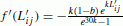
The marginal effects on property prices using the hedonic price function in Eq. 3 is given by:

where


and where prim denotes the first derivative. For each noise sources the marginal WTP is evaluated based on the mean value of the other variables. Equation 9 may therefore be written as:

where  is a constant. Index j denotes that this constant is dependent on the level of the other noise sources; that is, the constant varies between the noise variables.
As the estimates are to be used on a national level, the income differences between Lerum and the rest of the country should be taken into account. Corrections are based on the difference in income and empirically estimated income elasticities for the WTP for a noise reduction ( ). Let
  and
and  denote mean income for Sweden and Lerum, respectively, and the calculation model for the WTP then becomes:

where the equation is multiplied by −1 to give a positive value.
As the threshold value for when noise is regarded as disturbing is set at 50 dB in Sweden [65], our estimations are based on this value. The estimation of the annual social cost per person in the case of a change in level from  to
to  can then be estimated by:

where  and
and  are given by Eqs. 7 and 13. Hence, Eq. 14 assumes that the estimated WTP do not reflect the total social cost, since it includes
  to estimate
  . Therefore, by simply dropping
  from the equation we can estimate the total social cost under the assumption that WTP do indeed reflect the total social cost.
4.2 Abatement values for transport noise
As mentioned above, Eq. 12 should be turned into an annuity and the property tax and number of occupants of the property should be taken into consideration. Since estimations are sensitive to the choice of the discount factor, we choose to report calculations on three levels.Footnote 15 As a discount factor we choose the level 4 % as suggested by ASEK [65] for BCA in Sweden and for the sensitivity of our estimations we also show the results for 2 % and 6 %. The property tax in 2004 was 1.0 %, which is applied to 50 % of the value, and the number of occupants for our sample was, on average, 2.8 [56].Footnote 16
In order to transfer the results from Lerum to the rest of Sweden, differences in income between regions ought to be considered. Empirical estimations of income elasticity vary between 0.5–1.6 [5, 13, 44, 57, 69]. Since most of the estimations lie in the lower interval and nearer 1, we choose, like [44], to set  . This means that the values from Lerum should be multiplied by the actual quotient between the average incomes for Sweden and Lerum, which, for the age group 20 and over, was 0.875 during the data period (www.ssd.scb.se, 2008–11–19).
As explained, Eq. 14 should be used for “smaller changes”, i.e. for individuals’ preferences for marginal changes in noise level (not elimination). Table 3 contains some examples where the change is 1 dB. The choice of levels is based on the presentation in [19] and the estimates have been calculated without the health cost component to facilitate a comparison with other WTP studies. The constants reported in Table 3 are from Eqs. 11 and 13. This table reports the results of the sensitivity analysis for choice of discount factor, and as shown by the table, the values are sensitive to the choice of the discount factor.
Table 4 provides the comparison between the benefit measures of this paper and the three studies of interest described above. The benefit measures of this study (REBUS) which are estimated with Eq. 14 are shown with and without the health premium. As mentioned above, it was assumed that the earlier ASEK values, based on hedonic evaluation, did not reflect the whole social cost ([65], p. 119–120), and therefore, based on Danish findings [54, 55] the WTP estimates were adjusted upwards by 42 %. Since we suggest a constant marginal cost per dB for the health premium the percentage adjustment varies over the levels with the highest adjustment for lower levels, and by mode. Whereas the highest adjustment for road noise is 20 % it is considerably higher for rail noise, 300 %. Due to the convexity of cost function for rail noise it rapidly drops to 6 % and 2 % for the two highest levels in Table 4, though. Hence, the constant percentage adjustment is not supported by our findings, and the health premium is most significant at lower levels, especially for rail noise.
Our estimates (REBUS) are generally higher than the estimates from HEATCO and higher for road-traffic noise compared to [19]. Note that [19] finds a higher WTP to reduce railway noise than road noise. A suggested explanation for their results is too few observations for railway noise ([44], p. 334). A direct comparison between REBUS and ASEK is only relevant for road noise since there is no corresponding ASEK value for railway noise. Therefore, since the ASEK values include the health component we compare these values to the REBUS values also including the health component. These REBUS values indicate that the social cost of noise is underestimated at low levels with the current values, and substantially overestimated at higher levels. The strongly progressive relation in ASEK is not found in either HEATCO or in [19].Footnote 17 The relation between cost and noise level for railways in REBUS is similar to that in ASEK.
5 Discussion and conclusions
We have in this study estimated the social cost of road and rail traffic noise and described how WTP estimates from hedonic pricing studies can be combined with cost estimates for health effects in order for the estimates to reflect the total social cost. Based on estimates where the two cost components have been combined we find that the largest part of the social cost from noise exposure is the annoyance component, which is reflected in the individuals’ WTP. The WTP estimates in this study correspond with the annoyance relationship found in the acoustics literature; that is, the WTP is generally higher for reducing road than rail traffic noise. This is important from a validity perspective and our results show the need to revise the Swedish benefit measure of transport noise abatement in [65], which for all transport modes are based on WTP estimates for road noise. By using an unusually rich data set, in which we are able to estimate individuals’ WTP separately for road and railway noise, we show that WTP to reduce road and rail traffic noise not only differ in absolute but also marginal levels.
Our finding also show the importance of the chosen social discount rate. Even modest differences in the discount rates result in significant differences in the welfare estimates. Hence, the chosen discount rate by analysts or policy makers needs to be well motivated, to avoid values being tampered with. Regarding the second cost component, the unintended health effect, even if it is small relative to the WTP for most noise levels it is not negligible. For rail traffic and noise levels within the lower end of the interval it is either the dominant component or a relatively large share of it since here the welfare estimate of annoyance is low. Since most individuals live at the lower noise levels this has implications for a welfare analysis, such as BCA. For Swedish policy purposes we suggest that health costs should be evaluated by means of the impact pathway approach (IPA) since it is sanctioned in the EU, but more importantly, is superior to the alternative approach of relating the total estimated social cost to WTP estimates (as suggested by ASEK). More importantly, though, we believe that more research is necessary not only to study the relationship between annoyance and health effects, but also what effects are unintended and thereby not part of the individual’s WTP. The approach of adjusting the WTP estimates assumes that house owners are indeed unaware of the negative health effects and do not bear the full cost of noise related health effects. This is, as outlined above, in line with the general view among analysts and policy makers. However, as also pointed out, the empirical evidence is limited. Therefore, if evidence instead suggests that house owners are well informed, and that the COI related to these health effects is negligible, the estimates from the hedonic price regression analysis should be left unadjusted.
Estimated WTP in this study is based on actual decisions by house buyers and the estimates are adjusted based on income differences between the study area and the national level. The latter refers to the use of benefits transfer (BT) and it has been argued that evaluation in respect of BT should be based on annoyance, not dB, and done with SP-studies ([43], p. 30). The annoyance measure rather than dB is preferred simply because it can be evaluated with SP methods. The advantage of using an SP method is that it possible to establish the effect of the study design and individual characteristics on the results. However, the difficulty of estimating individuals’ preferences in SP studies is well established [9, 18] and we, therefore, do not agree that there is support that SP are superior to RP methods. Revealed preference methods are based on actual decisions, not hypothetical ones, and if, for instance, data is available to conduct the second step of the HP method [19, 44] it is possible to adjust the welfare measures based on results on individual characteristics from a RP study.
Today’s traffic noise policies are often influenced by guidelines for acceptable noise levels rather than welfare efficiency.Footnote 18 To gain acceptance for the use of BCA among policy makers it is therefore important not only to provide monetary welfare measures but also to inform about strengths and weaknesses, policy implications of using different values, and potential use. For instance, the belief that WTP estimates should be augmented with the health cost is widely held among many policy makers. We have shown how this can be done, but we have also highlighted that the evidence for doing so is weak. The policy implication of using today’s official values instead of the estimates of this study is the risk that social benefits from a road-noise-reducing measures will be underestimated, due to the strong progressive relationship between costs and noise levels and the fact that most people are subjected to low noise levels. Moreover, the choice of the recommended welfare measures is also important for the potential use of infrastructure user charges based on the marginal cost principle, since it has been shown these charges are determined largely by the individuals subjected to low noise levels [2, 3]. Evidence found in this and other studies need to be communicated by analysts to policy makers to secure a more efficient resource allocation. This study aims of doing this and has with a critical discussion of its results contributed to the estimation of the total social cost related to road and rail noise. There is, though, as has been highlighted need and room for further research.
Notes
Freely translated from Swedish, the acronym ASEK refers to “Working group for benefit-cost analysis”.
The financing of the COI related to noise is not directly linked to the exposed individuals, which could also motive adding a health cost component to the WTP estimate.
Let P and L denote property prices and noise level, respectively, then the NSDI is given by
Weaknesses of the SP-methods, such as insensitivity of the WTP to quantity of the good, hypothetical and strategic bias, anchorage effects and so on, are well known in the literature and may sometimes be a result of to poorly conducted studies (see, e.g., [9]).
The countries taking part were Norway, Spain, Sweden, Germany, the UK and Hungary. The Hungarian study also estimated values for air traffic noise.
Studies that look explicitly at the evaluation of rail traffic noise are few in number; [16] lists 4 hedonic and 2 SP studies, of which several are estimated according to distance from the railway rather than the noise level, or have other characteristics that make them less suitable for comparisons.
Nunes and Travisi [52] in addition to their own SP study also provide and overview of other SP studies.
For a description of this approach and the property tax effect on the evaluation, see e.g. [24].
For a more comprehensive description of the analysis and the results we refer to [1].
The total equivalent noise level was calculated as
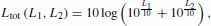
where
 , as before represents the equivalent noise level in dB from road (1) and rail (2) traffic noise, respectively.
Regression analysis was conducted using STATA. Andersson et al. [1] also presented results based on a semi-logarithmic form and conducted tests for spatial dependence, i.e. a violation of the independence between observation. They found strong evidence of a spatial dependence and the reason why the regression in Table 2 has not been tested for spatial dependence is because it is estimated with non-linear estimation and methods for incorporating spatial dependence in non-linear regressions have not been developed. Andersson et al. [1] also concluded that the spatial dependence would only have a negligible effect on the welfare estimates, hence the OLS and the spatial-lag model revealed similar estimates of marginal WTP. In addition they also examined the effect by using 55 dB as the threshold level, a level often used by authorities as a limit value below which no measures are taken to mitigate the noise [50]. They found that the results were sensitive to the threshold level chosen, a problem usually ignored in the literature where results based on only one level are reported.
Angelov [4] evaluates the health cost of road traffic noise with similar methods using data for the Swedish relationship from [36]. The risk of high blood pressure and coronary artery disease is calculated for the whole population. The results of the study should be “regarded as a calculation exercise” (p. 2, freely translated from Swedish [4]) but imply that previous ASEK values should be adjusted upwards by 60 % instead of the 42 % ASEK-choice based on the Danish studies.
Our main objective with this analysis is to show the sensitivity of the annual WTP to relatively small variations in the discount rate. We abstain from a broader discussion on the difficulties of choosing an appropriate discount rate and how to take into account uncertainty about the future, which instead can be found in [59].
The property tax is based on the property’s taxable value. The point of departure is that this value should constitute 75 % of the market value [62]. Data material from Lerum showed, though, a taxable value corresponding to 50 % of the market value.
A reason for this difference between ASEK and our results may be Wilhelmsson’s function-form combined with the fact that the study did not control for other negative effects of proximity to roads; that is, the marginal relation between costs and noise is probably overestimated at high noise levels using the current calculation values, a problem also noticed in ([72], p. 808).


 , as before represents the equivalent noise level in dB from road (1) and rail (2) traffic noise, respectively.
References
Andersson H, Jonsson L, Ögren M (2010) Property prices and exposure to multiple noise sources: hedonic regression with road and railway noise. Environ Resour Econ 45:73–89
Andersson H, Ögren M (2007) Noise charges in rail infrastructure: a pricing schedule based on the marginal cost principle. Transp Policy 14(3):204–213
Andersson H, Ögren M (2011) Noise charges in road infrastructure: a pricing schedule based on the marginal cost principle. J Transp Eng 137(12):926–933
Angelov EI (2008) Vägtransportsektorns folkhälsokostnader—en första ansats till samlad beräkning. Technical Report 2008:18, WSP Analys & Strategi, Stockholm
Arsenio E, Bristow AL, Wardman M (2006) Stated choice valuations of traffic related noise. Transp Res Part D Transp Environ 11(1):15–31
Babisch W (2011) Cardiovascular effects of noise. Noise Health 13(52):201
Babisch W, Bäckman A, Basner M et al (2011) Burden of disease from environmental noise. Bonn: WHO European Centre for Environment and Health
Bateman I, Day B, Lake I, Lovett A (2001) The effects of road traffic on residential property values: a literature review and hedonic pricing study. Technical report, University of East Anglia, Economic & Social Research Council, and University College London
Bateman IJ, Carson RT, Day B, Hanemann M, Hanley N, Hett T, Jones-Lee M, Loomes G, Mourato S, Özdemiroḡlu, Pearce DW, Sugden R, Swanson J (2002) Economic valuation with stated preference techniques: a manual. Edward Elgar, Cheltenham, UK
Beelen R, Hoek G, Houthuijs D, van den Brandt P, Goldbohm R, Fischer P, Schouten L, Armstrong B, Brunekreef B (2009) The joint association of air pollution and noise from road traffic with cardiovascular mortality in a cohort study. Occup Environ Med 66(4):243
Bickel P (2006) Derivation of fall-back values for impacts due to noise. Technical report, HEATCO (Developing Harmonised European Approaches for Transport Costing and Project Assessment)
Bickel P, Friedrich R, Burgess A, Fagiani P, Hunt A, Jong GD, Laird J, Lieb C, Lindberg G, Mackie P, Navrud S, Odgaard T, Ricci A, Shires J, Tavasszy L (2006) Proposal for harmonised guidelines. Deliverable 5, HEATCO (Developing Harmonised European Approaches for Transport Costing and Project Assessment)
Bjørner TB (2004) Combining socio-acoustic and contingent valuation surveys to value noise reduction. Transp Res Part D Transp Environ 9(5):341–356
Bluhm G, Nordling E (2005) Health effects of noise from railway traffic—the HEAT study. Inter-Noise
Boverket (2003) Buller: Delmål 3—Underlagsrapport till fördjupad utvärdering av miljömålsarbetet’. Boverket, Karlskrona
Brons M, Nijkamp P, Pels E, Rietveld P (2003) Railroad noise: economic valuation and policy. Transp Res Part D Transp Environ 8(3):169–184
Carlsson F, Lampi E, Martinsson P (2004) Measuring marginal values of noise disturbance from air traffic: does the time of day matter? Transp Res Part D 9(5):373–385
Carson RT, Flores NE, Meade NF (2001) Contingent valuation: controversies and evidence. Environ Resour Econ 19(2):173–210
Day B, Bateman I, Lake I (2007) Beyond implicit prices: recovering theoretically consistent and transferable values for noise avoidance from a hedonic property price model. Environ Resour Econ 37(1):211–232
de Vos P (2003) How the money machine may help to reduce railway noise in Europe. J Sound Vib 267(3):439–445
Dekkers J, van der Straaten JW (2009) Monetary valuation of aircraft noise: a hedonic analysis around Amsterdam airport. Ecol Econ 68(11):2850–2858
European Commission (1996) Future noise policy—European commission green paper. Report COM(96) 540 final, European Commission, Brussels, Belgium
European Communities (2002) Position paper on dose response relationships between transportation noise and annoyance. Technical report, Office for Official Publications of the European Communities, Luxembourg. ISBN 92-894-3894-0
Freeman AM (2003) The measurement of environmental and resource values. Washington, D.C., US: Resources for the Future, 2 edn.
Friedrich R, Bickel P (2001) Environmental external costs of transport. Springer Verlag, Heidelberg, Germany
Galilea P, Ortúzar JD (2005) Valuing noise level reductions in a residential location context. Transp Res Part D Transp Environ 10(4):305–322
Garrod GD, Scarpa R, Willis KG (2002) Estimating the benefits of traffic calming on through routes. J Transp Econ Policy 36(2):211–231
Hammar T (1974) Trafikimmisionens inverkan på villapriser. Statens Vägverk, Vägförvaltningen i Stockholms län, Mimeo
Hansson L (1995) Värdering av Trafikbuller. Bilaga till Samplan, SIKA Rapport 1995 14
ISO (2003) ISO/TS 15666 acoustics—assessment of noise annoyance by means of social and socio-acoustic surveys. Technical report, ISO
Jonasson H (2005) Svenska riktvärden och
 . Technical report ETaP404604 ver. 3, SP Akustik
Jonasson H, Nielsen H (1996) Road traffic noise—nordic prediction method. TemaNord 1996:525, Nordic Council of Ministers, Copenhagen, Denmark. ISBN 92-9120-836-1
Kalivoda M, Danneskiold-Samso U, Krüger F, Bariskow B (2003) EURailNoise: a study of European priorities and strategies for railway noise abatement. J Sound Vib 267:387–396
Kihlman T (2005) Developments in environmental noise policies.In: Proceedings of forum acusticum. Paper 964-0, Budapest, pp 35–40
Kihlman T, Wibe S, Johansson SM (1993) Priset på tystnad, en enkätstudie om människors värdering av bullerdämpande åtgärder.In: Bilaga 7, SOU 1993:65, Handlingsplan mot buller: Betänkande av Utredningen för en handlingsplan mot buller. Fritzes, Stockholm, Sweden
Kjellström K, Ferguson R, Taylor A (2008) Den svenska vägtransportsektorns folkhälsoeffekter
Li H, Chau C, TSE M, Tang S (2009) Valuing road noise for residents in Hong Kong. Transp Res Part D 14:264–271
Lindberg G (2007) Hälsoeffekter av buller. Appendix in “Värdering av bullerprofiler” 2007:27, WSP Analys & Strategi, Stockholm, Sweden
Lundström A, Jäckers-Cüppers M, Hübner P (2003) The new policy of the European Comission for the abatement of railway noise. J Sound Vib 267:397–405
Metroeconomica (2001) Monetary valuation of noise effects: final draft report. Mimeo May, Preparde for The EC UNITE Project
Miedema HME, Oudshoorn CGM (2001) Annoyance from transportation noise: relationships with exposure metrics DNL and DENL and their confidence intervals. Environ Health Perspect 109(4):409–416
Navrud S (2002) The state-of-the-art on economic valuation of noise: final report to European commission DG environment. Mimeo
Navrud S (2004) The economic value of noise within the European union—a review and analysis of studies. Mimeo
Nellthorp J, Bristow AL, Day B (2007) Introducing willingness-to-pay for noise changes into transport appraisal: an application of benefit transfer. Transp Rev 27(3):327–353
Nelson JP (1980) Airports and property values. A survey of recent evidence. J Transp Econ Policy 14(1):37–52
Nelson JP (2004) Meta-analysis of airport noise and hedonic property values. J Transp Econ Policy 38(1):1–28
Nelson JP (2008) Hedonic property values of studies of transportation noise: aircraft and road traffic. In: Baranzini A, Ramirez J, Schaerer C, Thalmann P (eds) Hedonic methods in housing markets: pricing environmental amenities and segregation. Springer, pp 57–82
Nielsen H (1996) Railway traffic noise—the nordic prediction method. TemaNord 1996:524, Nordic Council of Ministers, Copenhagen, Denmark. ISBN 92-9120-837-X
Nijland HA, Van Kempen EEMM, Van Wee GP, Jabben J (2003) Costs and benefits of noise abatement measures. Transp Policy 10(2):131–140
Nijland HA, Van Wee GP (2005) Traffic noise in Europe: a comparison of calculation methods, noise indices and noise standards for road and railroad traffic in Europe. Transp Rev 25(5):591–612
Niskanen WA, Hanke SH (1977) Land prices substantially underestimate the value of environmental quality. Rev Econ Stat 59(3):375–377
Nunes PA, Travisi CM (2007) Rail noise-abatement programmes: a stated choice experiment to evaluate the impacts on welfare. Transp Rev 27(5):589–604
Oertli J (2000) Cost-benefit analysis in railway noise control. J Sound Vib 231(3):505–509
Ohm A, Jensen MP (2003) Strategi for begræcnsning af vejtrafikstøj—Delrapport 3—Virkemidler og samfundsøkonomiske beregninger. Arbejdsrapport 54, Miljøstyrelsen, København
Ohm A, Lund SP, Poulsen PB, Jakobsen S (2003) Strategi for begrænsning af vejtrafikstøj—Delrapport 2—Støj, gener og sundhed. Arbejdsrapport 53, Miljøstyrelsen, København
Öhrström E, Skånberg A, Barreård L, Svensson H, Ängerheim P (2005) Effects of simultaneous exposure to noise from road and railway traffic. Inter-Noise
Palmquist RB (1992) Valuing localized externalities. J Urban Econ 31:59–68
Pearce D, Atkinson G, Mourato S (2006) Cost-benefit analysis and the environment: recent developments. OECD, Paris, France
Pindyck RS (2007) Uncertainty in environmental economics. Rev Environ Econ Policy 1(1):45–65
Prop 2008/09:35 (2001) Government bill 2008/09:35: Framtidens resor och transporter—infrastruktur för hållbart tillväxt. Government bill by the Swedish Government
Rosen S (1974) Hedonic prices and implicit markets: product differentiation in pure competition. J Polit Econ 82(1):34–55
SFS (2001) Fastighetstaxeringslag 1979:1152. 5 kap. 2 paragrafen, Lag (2001:1218), Finansdepartementet, Stockholm, Sverige
SIKA (1999) Översyn av samhällsekonomiska kalkylprinciper och kalkylvärden på transportområdet. SIKA Report 1999:6, SIKA (Swedish Institute for Transport and Communications Analysis), Stockholm, Sweden
SIKA (2005) Kan trafikbullerpolitiken göras mer effektiv?SIKA PM 2005:11, SIKA (Swedish Institute for Transport and Communications Analysis), Stockholm, Sweden
SIKA (2008) Samhällsekonomiska kalkylprinciper och kalkylvärden för transportsektorn. SIKA PM 2008:3, SIKA (Swedish Institute for Transport and Communications Analysis)
Sørensen M, Hvidberg M, Andersen Z, Nordsborg R, Lillelund K, Jakobsen J, Tjønneland A, Overvad K, Raaschou-Nielsen O (2011) Road traffic noise and stroke: a prospective cohort study. Eur Heart J 32(6):737–744
SOU (1993) Handlingsplan mot buller: Betänkande av Utredningen för en handlingsplan mot buller. SOU 1993:65, Statens offentliga utredningar, Miljö- och naturresursdepartementet, Stockholm, Sweden
Sydsæter K, Strøm A, Berck P (2000) Economists’ mathematical manual. Springer-Verlag, Heidelberg, Germany
Wardman M, Bristow AL (2004) Traffic related noise and air quality valuations: Evidence from stated preference residential choice models. Transp Res Part D Transp Environ 9(1):1–27
Wibe S (1997) Efterfrågan på tyst boende. A4 1997, Byggforskningsrådet, Stockholm, Sweden
Wilhelmsson M (1997) Trafikbuller och fastighetsvärden—en hedonisk prisstudie. Meddelande 5:45, Division of Building and Real Estate Economics, Royal Institute of Technology, Stockholm, Sweden
Wilhelmsson M (2000) The impact of traffic noise on the values of single-family houses. J Environ Plan Manag 43(6):799–815
 . Technical report ETaP404604 ver. 3, SP Akustik
Author information
Authors and Affiliations
Corresponding author
Additional information
This study was funded by SIKA and Banverket, and the financial support is gratefully acknowledged. Henrik Andersson is grateful for financial support from VTI and CTS (Stockholm). The authors are solely responsible for the results and views expressed in this paper.
Appendix: Descriptive statistics
Appendix: Descriptive statistics
Rights and permissions
Open Access This article is distributed under the terms of the Creative Commons Attribution 2.0 International License (https://creativecommons.org/licenses/by/2.0), which permits unrestricted use, distribution, and reproduction in any medium, provided the original work is properly cited.
About this article
Cite this article
Andersson, H., Jonsson, L. & Ögren, M. Benefit measures for noise abatement: calculations for road and rail traffic noise. Eur. Transp. Res. Rev. 5, 135–148 (2013). https://doi.org/10.1007/s12544-013-0091-3
Received:
Accepted:
Published:
Issue Date:
DOI: https://doi.org/10.1007/s12544-013-0091-3