

Abstract
Biases in climatological and extreme precipitation estimates are assessed for 11 global observational datasets constructed with merged satellite measurements and/or rain gauge networks. Specifically, the biases in extreme precipitation are contrasted with mean-state biases. Extreme precipitation is defined by a 99th percentile threshold (R99p) on a daily, 1° × 1° grid for 50 °S–50 °N. The spatial pattern of extreme precipitation lacks distinct features such as the ITCZ that is evident in the global climatological map, and the climatology and extremes share little in common in terms of the spatial characteristics of inter-product biases. The time series also exhibit a larger spread in the extremes than in the climatology. Further, when analysed from 2001 to 2013, they show relatively consistent decadal stability in the climatology over ocean while the dispersion is larger for the extremes over ocean. This contrast is not observed over land. Overall, the results suggest that the inter-product biases apparent in the climatology are a poor predictor of the extreme-precipitation biases even in a qualitative sense.
Export citation and abstract BibTeX RIS

Original content from this work may be used under the terms of the Creative Commons Attribution 3.0 licence. Any further distribution of this work must maintain attribution to the author(s) and the title of the work, journal citation and DOI.
Appendix: Glossary
| AMSR-E | Advanced Microwave Scanning Radiometer for EOS |
| CDR | Climate Data Record |
| CHIRPS | Climate Hazards Group InfraRed Precipitation with Station |
| CMORPH | CPC MORPHing technique |
| CM SAF | Satellite Application Facility on Climate Monitoring |
| CPC | Climate Prediction Center |
| DAPAGLOCO | Daily Precipitation Analysis for the validation of Global medium-range Climate predictions Operationalized |
| DMSP | Defence Meteorological Satellite Program |
| ENSO | El Niño Southern Oscillation |
| EOS | Earth Observing System |
| ETCCDI | Expert Team on Climate Change and Detection Indices |
| FROGS | Frequent Rainfall Observations on GridS |
| GPCC | Global Precipitation Climatology Centre |
| GPCP | Global Precipitation Climatology Project |
| GPM | Global Precipitation Measurement Mission |
| GSMaP | Global Satellite Mapping of Precipitation |
| HOAPS | Hamburg Ocean Atmosphere Parameters and Fluxes from Satellite Data |
| IMERG | Integrated Multisatellite Retrievals for GPM |
| PERSIANN | Precipitation Estimation from Remotely Sensed Information using Artificial Neural Networks |
| SSM/I | Special Sensor Microwave/Imager |
| SSMIS | Special Sensor Microwave Imager/Sounder |
| TAPEER | Tropical Amount of Precipitation with an Estimation of ERror |
| TRMM | Tropical Rainfall Measuring Mission |
1. Introduction
Accurately measuring precipitation on a global scale remains a challenge. The ground-based capability for monitoring precipitation is limited to the land portion of the Earth's surface. Most countries operate some form of rain-gauge network, but only a few countries have the opportunity to combine these with networks of local weather radars. The ground-based datasets used here rely on collections from these various networks of rain-gauges. Thus, they are limited to coverage over land, with some regions having relatively sparse coverage. Satellite observations offer a complementary means of precipitation measurements beyond the reach of in situ weather stations, but satellites estimates are not free of errors. Geostationary (GEO) satellites have the ability to uniformly and continuously monitor clouds, but not with an instrument sensitive to raindrops beneath the cloud layer they observe. Low Earth orbiting (LEO) spacecrafts carrying microwave instruments are superior in the detection skill of precipitating particles, but sample only intermittently and thus can miss important components of precipitation's inherent diurnal cycle or intense short-term events. Among the precipitation datasets widely adopted across the user community are 'merged' products constructed with different observations from multiple GEO and/or LEO satellites with or without gauge networks in the hope to compensate for the drawbacks inherent in individual observations (see section 2 for a list of such datasets).
Significant effort has been devoted to assess the consistency of these 'merged' precipitation datasets ([1–5] among others). Most of the work in this area, however, is focused on the 'mean' precipitation accumulation rather than the properties of the precipitation distribution itself. There exist some studies that focus on extreme precipitation at regional scales (e.g [6, 7]). Systematic assessments related to extremes on global scale, however, are few in the literature (e.g [8]). Yet, knowledge related to mean inter-product differences are not necessarily applicable to extremes, given that satellite-derived extreme precipitation is often associated with some cloud property (e.g. cloud top height or precipitation water content) rather than the intensity of precipitation itself [9].
The main goal of this article is a general description of inter-product precipitation biases for extreme precipitation as compared to the mean-state biases, providing a concise overview of the consistency among a broad range of global precipitation datasets in contrast to a large body of relevant work in the literature where selected products were examined in depth. The inter-comparison is made using different aspects of the precipitation such as precipitation histograms and global distribution patterns to identifying systematic similarities and differences among the products. The multi-year time series of precipitation are also intercompared and stability estimates are examined for the period of 2001–2013, for which a majority of the products currently analysed are available.
2. Data
In total, 11 products are selected for this work, consisting of 9 global multi-satellite datasets, with or without gauge calibration over land, and 2 gauge-based products used internally in some of those satellite products. The multi-instrument datasets included in this analysis are CMORPH v1.0 [10], GPCP v1.3 daily [11], GSMaP v6 [12], HOAPS v4.0 [13], IMERG v5 [14], PERSIANN-CDR v1r1 [15], TAPEER v1.5 [16], and TRMM 3B42 v7 [17]. Three land-only products, CHIRPS v2.0 [18], CPC v1.0 [19], and GPCC Full Data Daily v2018 [20, 21], are also analysed. All precipitation estimates are adjusted to a daily 1° × 1° grid, which accommodates the native resolution of all products in the current inventory. This choice is not necessarily optimal for assessing extreme precipitation [8] but is crucial to ensure the consistency in spatial and temporal resolutions for the inter-comparison. The statistical properties of extremes can be distorted for the most intense events when projected onto a coarse grid. As such, the current comparison may not precisely reflect the characteristics intrinsic of the original products at their native resolutions (see section 3.1). The product versions and resolution adopted here are fully compliant with the datasets stored in the FROGS archives [22]. Also, data from 2015 is not an official CM SAF HOAPS product and not part of FROGS. It was provided as a beta version of HOAPS version 4. We do not analyse all the products available from FROGS. The products on FROGS that are regional or ground-based without being used for any satellite-based dataset are outside our scope. Upstream products (e.g. microwave-only and no-gauge products) of 3B42, GSMaP, and CMORPH, regional products, and reanalysis precipitation are also not included in the current study.
CMORPH, GPCP, GSMaP, IMERG, TAPEER, and TRMM 3B42 are all constructed with satellite microwave and infrared measurements merged on a daily basis, where details of the merging techniques differ from one product to another. GSMaP, IMERG, and 3B42 each contain gauge-adjusted estimates over land, which are used in this study. GPCP daily precipitation is scaled to its monthly, gauge-calibrated product. PERSIANN-CDR is an infrared-based product adjusted to GPCP monthly precipitation. HOAPS precipitation is obtained from DMSP SSM/I and SSMIS observations over the global ice-free ocean. GPCC and CPC are gridded rainfall products constructed with data from gauge networks over the globe. CHIRPS is a satellite infrared-based product blended with station data.
IMERG is available only after the GPM launch in 2014, so we define the full year of 2015 as the reference period for detailed inter-comparisons. The time series analysis in section 3.3 is performed without IMERG. The latitudinal band of 50 °S–50 °N is analysed except for TAPEER (30 °S–30 °N) unless otherwise noted.
3. Climatology versus extremes
3.1. Histogram
Figure 1 shows log–log daily precipitation histograms computed from latitudinally-weighted statistics of daily values on a regular 1° × 1° grid for different datasets. The histogram is not normalised, so excesses and deficits do not cancel each other out. Nonetheless, the inter-product bias characteristics are inhomogeneous across magnitudes of precipitation. For instance, GPCP has higher frequency in the intermediate range of precipitation over ocean but quickly drops below all other datasets once daily precipitation exceeds approximately 30 mm d−1. In contrast, HOAPS has a large tail of high precipitation rates at the expense of a relatively low occurrence of intermediate precipitation. This demonstrates that biases in extremes can be fundamentally different from those that constitute the climatology (light and moderate precipitation). The spread among the products is smaller over land than over ocean.

Figure 1. Log–log daily precipitation histogram for global (50 °S–50 °N) precipitation over ocean (top) and over land (bottom).
Download figure:
Standard image High-resolution imageIt is noted that because precipitation estimates have been averaged onto a common 1° × 1° grid in figure 1, products with a higher native resolution would originally have a better capability of capturing extremes (figure S1 and table S1 is available online at stacks.iop.org/ERL/14/125016/mmedia in the supplementary material). Comparing figures 1 with S1 shows that the precipitation histograms at the original resolution are broadly spread across different products, where high-resolution datasets are indeed able to capture higher extremes. The spread is reduced with the signals of heaviest rains averaged out at the 1° × 1° resolution (figure 1). The inter-product spread, however, does not entirely vanishes, implying product-specific biases as described above.
In the figures that follow, extreme precipitation is defined by a 99th percentile threshold (or R99p according to the ETCCDI indices [23],) on a daily, 1° × 1° scale. We have tested the 30 and 20 mm d−1 thresholds for comparison (see the supplemental material). These two fixed-value thresholds correspond to different percentiles in the individual products and hence could potentially yield different extreme statistics from R99p. The zonal-mean extreme precipitation varies in a quantitative sense with threshold definitions, while the overall pattern stays qualitatively consistent among different thresholds.
3.2. Global distribution
Figure 2 shows the global distribution of the 2015 annual climatology of precipitation. Each product is presented as the anomaly field from the product ensemble mean (top left). Note that the magnitude of the anomaly field stays much smaller than the ensemble mean and all the products agree well in the general pattern as well as the zonal means (figures 4 and 5 below). Regional precipitation biases nonetheless show some interesting features. Oceanic precipitation from some products (GSMaP, HOAPS, and 3B42) is systematically higher in the ITCZ and lower in mid-latitudes than the ensemble mean, while others (CMORPH and IMERG) show contrasting spatial patterns in the anomaly field. Such a systematic bias pattern might be related to the built-in statistical relation of IR radiance with surface rainfall because dominant convective systems change from one region to the other. Deep organised systems are typical of the tropics while subtropical rainfall mostly comes from shallow cumulus. Mid-latitude storms are typically associated with synoptic-scale frontal systems. Otherwise it is not obvious why some products exhibit certain regional bias patterns given that the basic architecture of the retrieval algorithms is similar. Characteristic regionality in the global distribution of inter-product biases was also shown by [3]. Small-scale structures with alternating signs dominate outside the ITCZ in GPCP and PERSIANN.
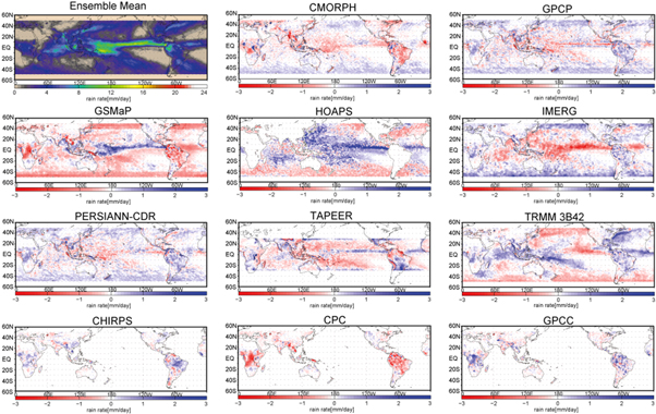
Figure 2. Product ensemble mean of 2015 annual precipitation climatology (top left) and anomaly from the ensemble for each product. TAPEER is not included in the ensemble mean because of the unavailability beyond 30° in latitude.
Download figure:
Standard image High-resolution imageAfrican and South American precipitation is either largely overestimated or underestimated depending on the products, with the consensus being poor even among the two gauge-based products (CPC and GPCC). The disagreement in the Congo is due largely to the known unavailability of data there in 2015 for GPCC and CPC, while origins of the discrepancy in South America are less clear. CMORPH, GPCP, GSMaP and PERSIANN exhibit a feature in the difference to the ensemble mean from 40 °S southward (GPCP and GSMaP also from 40 °N northward). This coincides with the transition from utilisation of GEO + LEO to LEO data.
The global distribution of extreme precipitation is qualitatively different from the climatology (figure 3). Subtropical bands of enhanced precipitation in the ensemble mean of extremes (top left) are in sharp contrast to the ITCZ, which stands out in the climatology. The spatial structure of extreme precipitation bias is more or less homogeneous although the sign and magnitude differs vastly among products. Figures 2 and 3 together show that extremes and climatology bear no apparent similarity in the geographical pattern either of the ensemble mean or the anomaly field.

Figure 3. As figure 2 but for extremes.
Download figure:
Standard image High-resolution imageTo summarise the inter-product differences, zonal mean precipitation climatology and extremes are plotted over the ocean in figure 4. While there is reasonable agreement for the climatology, different datasets have large differences in their extremes. The spread is relatively modest over land (figure 5) as expected from figure 1. Interestingly, most satellite-based products are bound between the two gauge products (CPC and GPCC) for the climatology over tropical land, presumably because the gauge network there is so sparse that two gauge products disagree from each other, depending sensitively on the choice of stations and interpolation schemes. The currently analysed version of GSMaP is heavily adjusted to the CPC product and closely follows the CPC rain in the zonal-mean climatology. Note that latitudes south of 45 °S over land consist almost solely of the southern tip of South America and suffer from larger statistical noise than other domains. Zonal-mean extremes with fixed rain-rate thresholds (20 and 30 mm d−1) exhibit qualitatively consistent spatial patterns in comparison with the R99p extremes although there are differences in absolute values (figures S2 and S3 in the supplementary material).

Figure 4. Zonal mean precipitation (2015 annual mean) over ocean for climatology (top) and extremes (bottom).
Download figure:
Standard image High-resolution image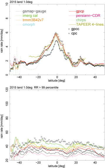
Figure 5. As in figure 4 but over land. The range for the ordinate is chosen to be identical to figure 4.
Download figure:
Standard image High-resolution image3.3. Time series
The analysis of time series is based on the same data records as in previous sections, i.e. data records from the FROGS archive [22]. The time series are computed either as weighted averages from daily values on a regular 1° × 1° grid per month or as 99th percentiles for a maximum period from January 1979—December 2018. Besides global means within 50 °N/S, means from three zonal bands are analysed: tropics within ±10°, northern hemisphere within 10 °N and 35 °N, and southern hemisphere within 10 °S and 35 °S. TAPEER does not fully cover these regions and is not part of the global analysis. Results related to the zonal bands are shown in the supplementary material. The averaged time series were further processed in two different ways: (1) For each individual data record, region, and metric (here, mean and 99th percentile), the following processing was applied: the climatological mean and annual cycle were computed. Then, the climatological annual cycle was removed. The resulting time series exhibits anomalies around a mean precipitation level of 0 mm d−1. Finally, the mean precipitation was added again. This approach was also applied by [24]. (2) For each region, for each metric and for the period January 2001—December 2013, the ensemble mean was computed. Then, the difference between each data record and the ensemble mean was normalised to the ensemble mean. This relative anomaly (or bias) time series is also used to estimate stability. Here, stability was computed as the change of the relative bias over the period 2001–2013 using a least absolute deviation method (adapted from the routine MEDFIT on page 703 in [25]). Associated uncertainties were computed following [26, 27] (see equation (6) of [27]). The null hypothesis is that the stability is different from 0%/decade and the alternative hypothesis is that the stability is not significantly different from 0%/decade. The null hypothesis is rejected if the coverage probability >95% (or p < 0.05).
We show results from approach (1) first, as this analysis is defined over the full temporal coverage of each data record. Figure 6 shows such time series for the global ocean and land within 50 °N/S. The vertical axis was optimised to allow a maximum zoom into the figure at the expense of a variable y-axis range. In general, the monthly means exhibit fairly good agreement over the ocean and only GSMaP is biased low. For the monthly means over land two clusters are evident corresponding to CPC and GPCC. Clustering around the gauge-based products may be partly explained by the gauge adjustment procedures: GPCP via its monthly adjustment, while 3B42 use a previous version of GPCC, GSMaP and CMORPH adopt CPC, PERSIANN was adjusted to GPCP monthly precipitation and CHIRPS utilises gauge data (see [28] for details on CHIRPS). The difference between the clusters is approximately 0.5 mm d−1 in the 2000s, associated with a bias between CPC and GPCC. This bias is smaller in the 1980s though. Over land PERSIANN exhibits good agreement with GPCP and GPCC, except prior to the late 1980s. Furthermore, it can be seen that monthly means of HOAPS exhibit anomalies that coincide with ENSO variability. For PERSIANN, anomalies in May and June 1984 and June and July 2017 are evident. These anomalies coincide with systematic regional data gaps over Africa, Europe, and the Indian Ocean (May and June 1984) and anomalously low precipitation over the ITCZ in June and July 2017.
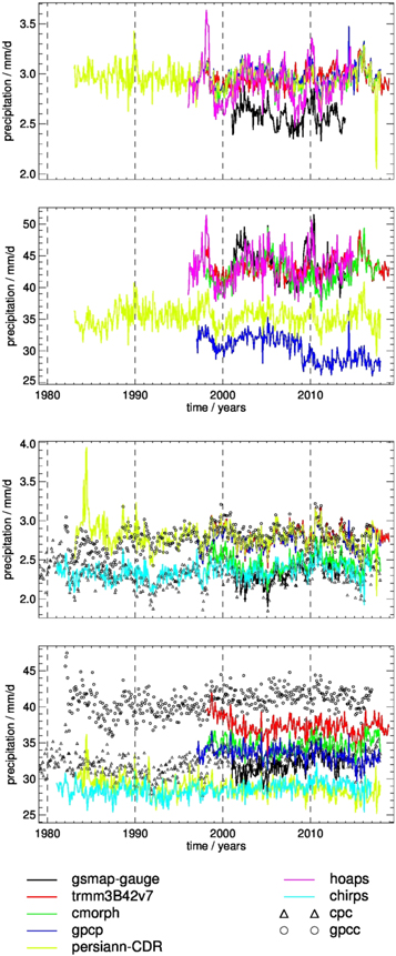
Figure 6. Time series of monthly mean precipitation with the annual cycle being removed: global ocean (top two panels) and global land within 50 °N/S (bottom two panels), mean over all defined values (first and third panel), and 99th percentile (second and fourth panel).
Download figure:
Standard image High-resolution imageThe results for the 99th percentile exhibit less agreement, i.e. a larger spread, and a lower level of clustering than for mean precipitation. In particular, the clustering around GPCC and CPC is no longer evident. Over the ocean, maximum 99th percentiles of precipitation are similar among 3B42, CMORPH, GSMaP and HOAPS while GPCP exhibits minimum 99th percentiles. An apparent jump to lower 99th percentiles for GPCP over the ocean occurs in late 2008/early 2009. It is noteworthy as it is not present in the other data records. Within GPCP the utilisation of SSM/I data ends in December 2008 and transfers to SSMIS in January 2009 [25]. For the GPCP Daily analysis the SSMI/SSMIS data is used to establish a precipitation frequency or precipitation/no precipitation threshold, with mean precipitation intensity determined by the GPCP monthly precipitation. This produces a conservative 99th (and other high percentile) values. The 2009 shift is likely related to a slight shift in that SSMI/SSMIS precipitation threshold that went undetected. This discontinuity may be sensitive to the threshold for extremes and needs further investigation. Over land 99th percentiles are lowest for PERSIANN and CHIRPS and highest for GPCC, with peak values in early 1982. This maximum coincides with the eruption of El Chichon in March 1982. However, values for January and February 1982 are the second and third highest values. Finally, a decrease in the 99th percentile of 3B42 over land between the start of the time series and 2005 is observed which is not evident in the other data records.
Results shown in figure 6 are discussed further because several minima and maxima of globally (within 50 °N/S) averaged values coincide with ENSO: Maxima and minima in mean precipitation and in 99th percentiles over the ocean are observed in 1998, 2010 and 2016 as well as in 1999, 2008 and 2011, corresponding to El Niño and La Niña events, respectively. Mean precipitation minima over land coincide with El Niño events in 1983, 1992, 1997, and 2016. Maxima are present in 1999/2000 and 2010/2011, coinciding with La Niña events. It is noticeable that the 99th percentiles over land do not exhibit minima/maxima in coherence with ENSO. The imprint of ENSO on precipitation was discussed, e.g. in [29, 30] and the contrasting behaviour in mean precipitation between land and ocean was also described, e.g. by [30] [31]. identified the impact of El Chichon and Pinatubo as minima in 1983 and 1991 in precipitation from GPCP [29]. observed coherent variability between precipitation extremes and ENSO over the tropical ocean and increased amplitudes of this variability with increasing percentiles [32]. emphasised that the response of precipitation to ENSO has a strong regional imprint which can locally exceed the expectation from Clausius–Clapeyron due to amplifications of ENSO dynamics by atmospheric feedbacks. They further concluded that the response of precipitation in the warm, moist ENSO regions is similar to the extreme response discussed in [29] while the tropic-wide response to ENSO is small due to compensating moistening and drying effects. Results from analysis of scaling or regression between precipitation and sea surface temperature data can be found in papers mentioned above and in particular in [33] who also utilised data records from FROGS. Note that the minimum in mean precipitation over land in 2005 does not correlate with ENSO or volcanoes. At present, this anomaly cannot be explained. Finally, it is noted that results presented in sections 3.1 and 3.2 are affected by the El Niño in 2015/2016. The observed response of HOAPS to ENSO partly explains the observed behaviour presented in these previous sections.
Time series of anomalies relative to the ensemble mean for the global ocean and land within 50 °N/S are shown in figure 7. Overall features are fairly similar to results shown in figure 6. This is in particular valid for the overall agreement in mean precipitation over the ocean, the clustering in mean precipitation over land and the larger spread in biases for 99th percentiles than for mean precipitation. To some extent the small bias among the mean precipitation over ocean can be explained with the adjustment of PERSIANN and CMORPH to GPCP (the latter over ocean only, see [34]). Maximum temporal variability in mean precipitation over ocean is observed for HOAPS and 3B42, with opposing minima and maxima between both data records reflecting maximum difference in the response to ENSO. The 99th percentile anomaly of CHIRPS over land exhibits a pronounced annual cycle. This indicates that CHIRPS exhibits the largest amplitude of the annual cycle. While hardly evident in figure 6, it can be seen in figure 7 that CHIRPS and CMOPRH are not closely following the 99th percentile anomaly of CPC over land.

Figure 7. Time series of anomalies relative to the ensemble mean for the period 2001–2013: global ocean (top two panels) and global land within 50 °N/S (bottom two panels), mean over all defined values (first and third panel), and 99th percentile (second and fourth panel).
Download figure:
Standard image High-resolution image
Stability estimates were computed for all time series shown in figure 7 with results provided in table 1. The spread in stability estimates over the ocean is fairly small, with generally non-significant differences among the products. An exception is the stability of 3B42. Prior to 2008 3B42 anomalies are smaller compared to the period after 2010 (see figure 7). In June 2009 elements of the precipitation hardware of TRMM were switched from nominal to back-up (https://pmm.nasa.gov/sites/default/files/document_files/TRMMSenRevProp_v1.2.pdf). However, a clear temporal coincidence between a jump in anomalies and this event is not evident. Stability estimates for 99th percentiles over ocean exhibit a larger spread with values ranging from −6.7%/decade (GPCP) to 7.4%/decade (3B42). Here, stability estimates are generally significantly different. GPCP exhibits the largest difference in stability between mean precipitation and the 99th percentile: while the mean precipitation of GPCP exhibits the highest level of stability, the low stability of the 99th percentile time series is explained by the jump in that time series occurring in late 2008/early 2009 (see second panel of figures 6 and 7). As mentioned earlier, this jump coincides with the change in the utilisation of SSM/I and SSMIS data.
Table 1. Stability estimates and associated uncertainties for global means and 99th percentiles within ±50° over ocean and land. Significant stability estimates are printed bold. Due to the limited temporal coverage (2001–2013) and the utilisation of the ensemble mean as reference the stability is only an estimate of the true stability.
| Global ocean | ||
|---|---|---|
| Stability/%/decade | ||
| Dataset | Global mean | 99th percentile |
| GPCP | −0.7 ± 0.35 | −6.7 ± 0.87 |
| HOAPS | −1.3 ± 0.75 | 3.6 ± 0.60 |
| 3B42 | 5.5 ± 0.75 | 7.4 ± 0.75 |
| CMORPH | −0.8 ± 0.29 | −3.7 ± 0.72 |
| PERSIANN | −2.1 ± 0.34 | 1.8 ± 0.39 |
| GSMaP | −1.1 ± 0.54 | −1.9 ± 1.10 |
| Global land | ||
| Dataset | Stability/%/decade | |
| Global mean | 99th percentile | |
| GPCC | −3.1 ± 0.69 | 0.0 ± 0.44 |
| CHIRPS | 0.3 ± 0.55 | 0.8 ± 1.00 |
| CPC | 2.5 ± 0.87 | 2.1 ± 0.69 |
| GPCP | −1.5 ± 0.41 | −4.0 ± 0.58 |
| 3B42 | −0.2 ± 0.43 | −1.0 ± 0.43 |
| CMORPH | 1.5 ± 0.56 | 0.0 ± 0.69 |
| PERSIANN | −2.5 ± 0.51 | −2.8 ± 0.43 |
| GSMaP | 5.3 ± 0.52 | 4.3 ± 0.35 |
The stability estimates for mean precipitation over land exhibit a fairly small spread, though with quite a few significant differences. CHIRPS, CMORPH and GPCC exhibit non-significant and low stability estimates while the stability estimate of GSMaP (5.3% ± 0.52%/decade) is the largest observed estimate over land. GPCP and GSMaP show maximum absolute stability estimates for 99th percentiles over land. The spread in 99th percentiles is smaller for land-based results than the equivalent ocean-based values. A possible explanation could be the direct or indirect use of rain gauges in the various products. While differences still exist because of the way the rain gauges are incorporated into products, an overall reduction in the land-based variability is not surprising.
It is emphasised that the ensemble mean contains contributions from all data records, including artificial trends and anomalies. Thus, the above stability discussion cannot address the true stability of the data records. However, the presented stability results allow the identification of stability issues in a relative sense and support the identification of spurious changes in the mean relative bias.
4. Discussion and summary
This work highlights precipitation differences among global gridded products in terms of regional patterns and multi-year time series, with a focus on the qualitative contrast between climatology and extremes. Precipitation extremes are defined by the 99th-percentile threshold (R99p) on a daily 1° × 1° grid. All products agree on some fundamental characteristics of extremes, such as subtropical maxima over ocean. On the other hand, the inter-product spread is significantly larger for extremes than for climatology particularly over the ocean, perhaps because there are no rain gauges available to bias-correct products. This suggests the importance of analysing multiple precipitation products at a time instead of relying on a single, arbitrarily chosen, product.
Although this article is not intended to rank the products for accuracy, it would be beneficial to comment on potential issues or strengths of selected datasets. HOAPS exhibits anomalies which coincide with ENSO but are in contrast to 3B42 anomalies. Figures S6–S8 of the supplement show that the ENSO response of HOAPS is dominated by observations over the tropics within 10 °N/S. Input observations for HOAPS are obtained exclusively from the SSM/I and SSMIS sensors. When using the DAPAGLOCO dataset (DOI:10.5676/DWD_CDC/HOGP_100/V002) which utilises SSM/I, SSMIS, AMSR-E and TMI observations and the HOAPS retrieval [13], the mean precipitation over the global ice-free ocean is similar between the HOAPS and the DAPAGLOCO products (not shown), with slightly smaller anomalies during La Niña events. Thus, the temporal sampling in HOAPS only partly explains HOAPS' ENSO response, i.e. the sensitivity of the retrieval needs to be examined in order to understand this feature. Over oceans, GSMaP exhibits the lowest mean precipitation. In figures S6–S8 of the supplement GSMaP is characterised by only slightly lower mean precipitation over the tropics and the northern and southern hemisphere up to 35 °N/S than the other data records. Thus, the reason for the bias observed in figure 6 must mainly be caused by observations beyond 35 °N/S. For 2015, zonal means of GSMaP exhibit minimum mean precipitation beyond ∼40 °N/S (figure 4) and it seems that this is valid more generally for the considered period.
GPCP precipitation is distinctly lower for extremes over the ocean than any other product analysed. Furthermore, GPCP exhibits a jump to lower 99th percentiles over the ocean in late 2008/early 2009, coinciding with the change in utilisation of SSM/I and SSMIS data. The potential negative bias and jump in GPCP extremes does not have any visible impact on the climatology. GPCP, whose main scopes include the construction of a reliable climate data record (CDR), has been developed with priority given to the stability of data over years [35]. The presented results indicate that this might not apply to extremes. Certain products, on the other hand, are not intended for CDRs but may be targeted more on high-resolution mapping of precipitation. The product users are advised to bear in mind that some products are tailored for specific purposes and may not necessarily be optimal for all applications.
Acknowledgments
H Masunaga and F A Furuzawa acknowledge support by JSPS KAKENHI Grant Number 19H05704 and JAXA and M Schröder acknowledges the financial support by the EUMETSAT member states through CM SAF. We are grateful to Bob Adler and two anonymous reviewers for their helpful comments.
Data availability statement
The data that support the findings of this study are openly available at https://doi.org/10.14768/06337394-73A9-407C-9997-0E380DAC5598 [22].