On the Adequacy of Representing Water Reflectance by Semi-Analytical Models in Ocean Color Remote Sensing


1
Scripps Institution of Oceanography, University of California, San Diego, 9500 Gilman Drive, La Jolla, CA 92093, USA
2
HYGEOS, Euratechnologies, 165 Avenue de Bretagne, 59000 Lille, France
*
Author to whom correspondence should be addressed.
Remote Sens. 2019, 11(23), 2820; https://doi.org/10.3390/rs11232820
Submission received: 29 October 2019
/
Revised: 21 November 2019
/
Accepted: 22 November 2019
/
Published: 28 November 2019
Abstract
:Deterministic or statistical inversion schemes to retrieve ocean color from space often use a simplified water reflectance model that may introduce unrealistic constraints on the solution, a disadvantage compared with standard, two-step algorithms that make minimal assumptions about the water signal. In view of this, the semi-analytical models of Morel and Maritorena (2001), MM01, and Park and Ruddick (2005), PR05, used in the spectral matching POLYMER algorithm (Steinmetz et al., 2011), are examined in terms of their ability to restitute properly, i.e., with sufficient accuracy, water reflectance. The approach is to infer water reflectance at MODIS wavelengths, as in POLYMER, from theoretical simulations (using Hydrolight with fluorescence and Raman scattering) and, separately, from measurements (AERONET-OC network). A wide range of Case 1 and Case 2 waters, except extremely turbid waters, are included in the simulations and sampled in the measurements. The reflectance model parameters that give the best fit with the simulated data or the measurements are determined. The accuracy of the reconstructed water reflectance and its effect on the retrieval of inherent optical properties (IOPs) is quantified. The impact of cloud and aerosol transmittance, fixed to unity in the POLYMER scheme, on model performance is also evaluated. Agreement is generally good between model results and Hydrolight simulations or AERONET-OC values, even in optically complex waters, with discrepancies much smaller than typical atmospheric correction errors. Significant differences exist in some cases, but having a more intricate model (i.e., using more parameters) makes convergence more difficult. The trade-off is between efficiency/robustness and accuracy. Notable errors are obtained when using the model estimates to retrieve IOPs. Importantly, the model parameters that best fit the input data, in particular chlorophyll-a concentration, do not represent adequately actual values. The reconstructed water reflectance should be used in bio-optical algorithms. While neglecting cloud and aerosol transmittances degrades the accuracy of the reconstructed water reflectance and the retrieved IOPs, it negligibly affects water reflectance ratios and, therefore, any variable derived from such ratios.
1. Introduction
Ocean color depends on the absorption and scattering properties of the constituents of the water body. Observation of spectral water reflectance from space is a major tool to gather information about water constituents and associated biogeochemical processes such as primary production. A number of atmospheric correction algorithms have been proposed to remove the influence of the atmosphere and surface in the satellite imagery and, therefore, retrieve the water signal (see e.g., [1]). One approach is to determine simultaneously the key properties of aerosols and water constituents of the coupled system by obtaining a best fit to the measured top-of-atmosphere (TOA) reflectance [2,3,4,5,6]. The advantage of this approach, compared with the standard two-step algorithm first suggested by [7], resides in its ability to manage situations of both Case 1 and Case 2 waters, i.e., waters whose inherent optical properties (IOPs) are either dominated by phytoplankton or markedly influenced by other constituents (colored dissolved organic matter and inorganic mineral particles), respectively, but this requires that the selected water reflectance model should be able to represent well the bio-optical variability across diverse aquatic ecosystems. Such atmospheric correction algorithms, whether deterministic or statistical, often use a simplified water reflectance model, such as the three-component model of Sathyendranath et al. [8], so that the absorption and scattering coefficients of the ocean water can be specified by a few parameters (e.g., chlorophyll concentration, backscattering and absorption coefficients at a given wavelength). The model, however, may not be representative of worldwide water conditions [9,10,11,12], since many variables affecting reflectance are fixed at some average values. It is generally preferable to make no assumption about the variable to retrieve. Such model may affect the retrieval of water reflectance and the accuracy of the derived ocean color products.
Steinmetz et al. [13] developed an algorithm called POLYMER to perform atmospheric correction in regions affected by sun glint and retrieve the spectrum of water reflectance. The POLYMER algorithm relies on two models: one is a simple polynomial atmospheric model fitting the scattering of the atmosphere and sun glint signal, and the other is a bio-optical water reflectance model. A spectral matching method is used to obtain the best fit of the TOA reflectance, and the water reflectance model parameters are retrieved in an iterative process. The POLYMER algorithm works effectively in the presence of Sun glint and thin clouds, increasing the useful coverage of satellite measurements. The European Space Agency (ESA) has selected POLYMER for operational generation of OC-CCI (Ocean Colour Climate Change Initiative) products [14,15]. One can choose from two water reflectance models in the POLYMER code: A modified version of the semi-analytical model of Morel and Maritorena [16], denoted MM01, and the semi-analytical model of Park and Ruddick [17], denoted PR05. The PR05 model is used as default in the latest version of the POLYMER code and the MM01 model is provided for optional usage. The MM01 model, slightly modified, depends on chlorophyll-a concentration and a backscattering coefficient for non-algal particles. The PR05 model depends on chlorophyll-a concentration, a parameter specifying the contribution of algal and non-algal particles to the backscattering coefficient, and a parameter allowing different absorption coefficients for dissolved organic matter. Accurate representation of the water reflectance is crucial to the success of the POLYMER algorithm. The adequacy of those models, therefore, needs to be assessed.
The objective of this study is to examine MM01 and PR05 in terms of their ability to represent properly water reflectance in a POLYMER-type inversion scheme applied to typical ocean-color sensors measuring in the spectral range 400–900 nm. The models are first evaluated theoretically, using Hydrolight simulations with IOPs specified from an IOCCG synthesized dataset [18], and then experimentally, using AERONET-OC measurements [19]. For this, POLYMER is applied to the simulated data or the measurements assuming no interference of the atmosphere and/or surface. The accuracy of the reconstructed water reflectance is quantified, as well as its influence on the derived IOPs using the Quasi-Analytical Algorithm (QAA) [20]. The impact of cloud and aerosol transmittance on the retrieval of water reflectance, neglected in POLYMER, is also evaluated.
2. Materials and Methods
2.1. Reflectance Models
The original MM01 model [16] is slightly modified by taking into account the absorption and backscattering of non-algal particles. The MM01 model uses two parameters: the chlorophyll-a concentration ([Chla]) and the backscattering coefficient of non-algal particles (bbs), which varies spectrally in λ−1 (λ is the wavelength). This allows applicability to Case 2 water situations. The model input also includes sun and sensor viewing geometry and wind speed. Specifically, the input geometry was set to match that of the specific dataset described later and the default value of wind speed was used, i.e., 5 m/s, as done in POLYMER. The output of this model is the spectral irradiance reflectance just below the surface, from which remote sensing reflectance, Rrs, is deduced. In the transformation, the f/Q correction is performed according to Morel and Gentili [21]. The similarity spectrum of Ruddick et al. [22] is used to extend the model from 700 to 900 nm.
The PR05 model is built from radiative transfer simulations for a wide range of IOPs that cover both Case 1 and Case 2 waters [17]. It is based on a generic parameterization of reflectance as a function of the total backscattering coefficients over the sum of the total absorption coefficients and the total backscattering coefficients. The PR05 model depends on three parameters: [Chla], a phase function parameter defined by the contribution of suspended particles to the backscattering coefficient (fb), and a parameter allowing different absorption coefficients for dissolved organic matter (fa). In POLYMER the default setting of the PR05 model is using [Chla] and fb as free parameters and fixing fa to 1. In this study, the PR05 model with both two and three free parameters was evaluated. Raman scattering is taken into account in the variant used, by applying Raman correction coefficients from Westberry et al. [23]. The model input also includes sun and sensor viewing geometry, which were set to match the geometry of the specific dataset described later. The default wind speed is 5m/s. The output of this model is the spectral bidirectional water reflectance just above the surface (Rw), defined as πLw/Ed where Lw is water-leaving radiance and Ed the downward solar irradiance just above the surface, from which Rrs = Lw/Ed is deduced by dividing by π.
2.2. Inversion Scheme
The model parameters, i.e., [Chla] and bbs in MM01, and [Chla], fa, and fb in PR05, are obtained from the prescribed Rrs at a set of wavelengths in the 400–900 nm spectral range using, as in POLYMER, the Nelder–Mead optimization scheme [24]. A simplex method is used to minimize the cost function f, which is defined as:
where Řrs(λi) is the modeled remote sensing reflectance at wavelength λi, and Rrs(λi) is the Hydrolight simulated or field measured remote sensing reflectance at wavelength λi. For the MM01 model, the first iteration simplex is defined by initial values log10([Chla]) = −1 and bbs = 0, and initial steps 0.05 and 0.0005 m−1. For the PR05 model, the first iteration simplex is defined by initial values log10([Chla]) = −1, log10(fb) = 0 and initial steps 0.2 and 0.2 when using two parameters, or by initial values log10([Chla]) = -1, log10(fb) = 0, log10(fa) = 0 and initial steps 0.2, 0.2, and 0.2 when using three parameters. The optimization scheme stops when f reaches a threshold value of 0.005 or the iteration reaches a maximum number.
f = ∑ (πŘrs(λi) − πRrs(λi))2/norm, norm = 0.005 if πRrs(λi) < 0.005, otherwise norm = πŘrs(λi),
2.3. Data Source
Two datasets were used in this study to evaluate the performance of the MM01 and PR05 water reflectance models, i.e., their ability to properly reconstruct a prescribed water reflectance spectrum. One dataset was obtained from radiative transfer simulations, the other from measurements at a variety of coastal sites.
The first dataset contained 500 cases generated using Hydrolight. These cases cover a wide range of Case 1 and Case 2 waters, but do not include extremely turbid water situations, such as those encountered in estuaries and inland water bodies. The simulations were made from 300 to 900 nm at 10 nm intervals. The input data including the IOPs and concentrations of phytoplankton, colored dissolved organic matter (CDOM), and detritus/minerals were taken from the synthesized dataset from IOCCG Report 5 [18]. The IOCCG synthesized dataset only provides IOPs at the wavelength range of 400–800 nm at 10 nm intervals. To extend the IOP values to the wavelengths below 400 nm (necessary to account for Raman scattering) and above 800 nm the following procedures were applied:
- Phytoplankton absorption. The phytoplankton absorption, aph, is expressed as aph = [Chla] a*ph, where a*ph is the chlorophyll-specific absorption coefficient, both provided in the IOCCG dataset. The values of a*ph at 350–400 nm were adopted from Morel [25] and extrapolated to 300 nm, which was then normalized to the IOCCG a*ph value at 400 nm to ensure continuity. The a*ph values in the 800-900 nm range were assumed constant and fixed at the value at 800 nm.
- CDOM absorption. The CDOM absorption, ag, was modeled as ag(λ) = ag(440) exp(−Sg(λ − 440)), with Sg and ag(440) provided by IOCCG [18].
- Detritus/mineral absorption. The absorption of detritus/mineral, adm, was modeled as adm(λ) = adm(440) exp(−Sdm(λ − 440)), with Sdm and adm(440) provided by IOCCG [18].
- Backscattering of phytoplankton. The attenuation of phytoplankton, cph, was modeled as cph = cph(550) (550/λ)n1 in the IOCCG dataset. The value of n1 was determined using cph at 400–800 nm, which was then used to extend cph to 300-1000 nm. The backscattering of phytoplankton, bbph, was thus obtained using bbph = ph(cph − aph) with ph equal to 0.01.
- Backscattering of detritus, mineral, and other particles. The backscattering of detritus, mineral, and others, bbdm, was modeled as bbdm = bbdm(550) (550/ λ)n2. The value of n2 was determined using bbdm at 400–800 nm, which was then used to extend bbdm to 300–900 nm.
All simulations were done with a solar zenith angle of 30° and a wind speed of 5 m/s. Pure seawater properties were specified by Pope and Fry [26] and Smith and Baker [27] for absorption and scattering, respectively. Clear sky condition and infinitely deep homogeneous water were assumed. The direct and diffuse solar irradiance were simulated using a semi-empirical sky model [28] with the annual average sun-earth distance and ozone content of 300 DU as input. Raman scattering and chlorophyll and CDOM fluorescence were also included in all simulations. The simulated nadir-viewed remote sensing reflectance, Rrs, was further interpolated into MODIS wavelengths (412, 443, 488, 531, 547, 667, 678, 748, and 869 nm). Note that the IOCCG synthesized IOPs do not cover all possible natural waters. However, as the models and parameters of describing input IOPs are based on extensive field measurements of oligotrophic and eutrophic waters [8,29,30,31,32,33,34,35], the Hydrolight simulated data should be consistent with a wide range of field observations.
The second dataset originated from the ocean color component of the Aerosol Robotic Network (AERONET-OC), which provides consistent and accurate long-term measurements collected by globally distributed autonomous radiometer systems deployed on offshore fixed platforms [19]. In the AERONET-OC dataset, the normalized water-leaving radiance LWN(λ) at various wavelengths in the visible and near-infrared spectral regions is the primary ocean color radiometric product. Data at quality-assurance level 2.0, normalized to the geometry of the Sun at zenith and the view at nadir, was used. The level 2.0 data is fully quality controlled including pre- and post-field calibration with differences smaller than 5%, automatic cloud removal, and manual inspection. Conversion to Rrs was accomplished by multiplying LWN(λ) by extraterrestrial solar irradiance. Note that uncertainties in the AERONET-OC in-situ measurements are about 5% in the blue to green bands, and about 8% in the red band [19]. The AERONET-OC measurements were collected using different radiometric instruments and thus the wavelengths used were not exactly the same. Since in this study Rrs at MODIS wavelengths (see above) are considered, and since the simulated data set corresponds to those wavelengths, measurements at wavelengths located within the MODIS center wavelengths ± 3 nm were selected. At some of the AERONET-OC sites, in particular the Venise site (45°N,12°E), measurements at 547 ± 3 nm were missing. In the end measurements from a total of fourteen sites were used, including twelve coastal sites, i.e., COVE_SEAPRISM (36°N, 75°W), Gageocho_Station (33°N,124°E), Ieodo_Station (32°N,125°E), Socheongcho (37°N,124°E), Galata_Platform (43°N,28°E), GOT_SEAPRISM (9°N,101°E), LISCO (43°N,70°W), Lucinda (18°S,146°E), Thornton_C-Power (51°N,2°E), USC_SEAPRISM (33°N,118°W), WaveCIS_site_CSI_6 (28°N,90°W), and Zeebrugge-MOW1 (51°N,2°E), and two lake sites, i.e., Lake_Erie (41°N,83°W) and Palgrunden (58°N, 13°E). Additional criteria based on the similarity spectrum [22] were applied to check and remove outliers, i.e., only the data for which (i) Rrs(869 nm) > −0.0001 sr−1 and (ii) the ratio Rrs(667 nm)/Rrs(869 nm) > 3 if Rrs(869 nm) >0.0008 sr−1 were selected. This resulted in a total number of 9824 Rrs measurements at wavelengths close to the MODIS wavelengths. For simplification, the AERONET-OC wavelengths will be referred to as 412, 443, 488, 531, 547, 667, and 869 nm, i.e., the MODIS wavelengths. The AERONET-OC measurements were made only under clear sky conditions. They were collected when wind speed is less than 15 m/s. Chlorophyll-a concentrations are provided in the AERONET-OC dataset, but not from field measurements; they are estimated through an iterative procedure making use of reflectance band ratios [19]. AERONET-OC sites for which band-ratio algorithms exist naturally benefit from those regional algorithms. For several AERONET-OC sites, the lack of regional algorithms imposes the application of the standard OC2V4 band-ratio. Because of this, the expected accuracy of AERONET-OC [Chla] varies from site to site.
3. Results and Discussion
3.1. Model Performance with Hydrolight Simulations
Model performance (MM01, PR05) was first evaluated theoretically using the Hydrolight simulations. Prior to evaluation, Case 1 and Case 2 waters were separated. Distinguishing Case 1 and Case 2 waters was based on the criteria proposed by Morel and Bélanger [36] and Robinson et al. [37]. According to Morel and Bélanger [36], the particulate scattering coefficient at 560 nm, bp(560), increases with increasing [Chla]. The upper limit of bp(560) can be expressed as
bp(560) = 0.69 [Chla]0.766
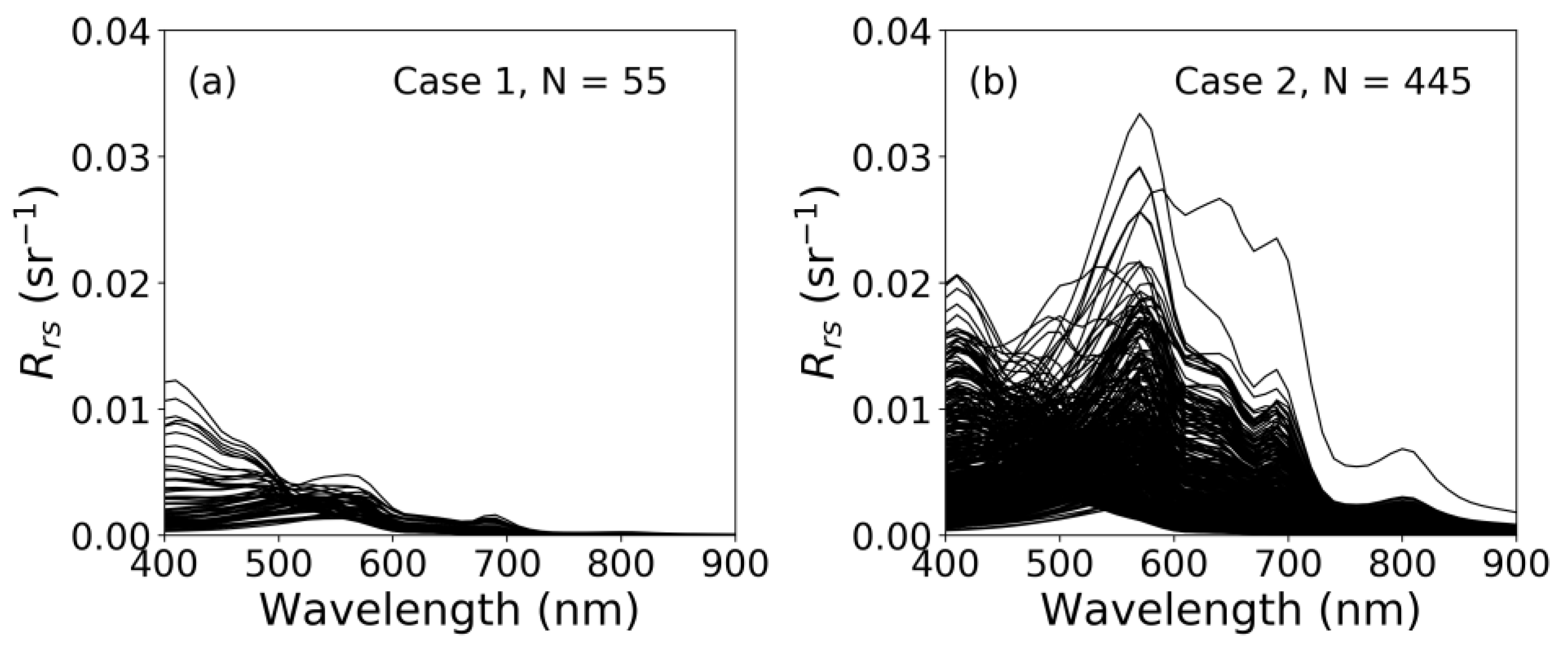
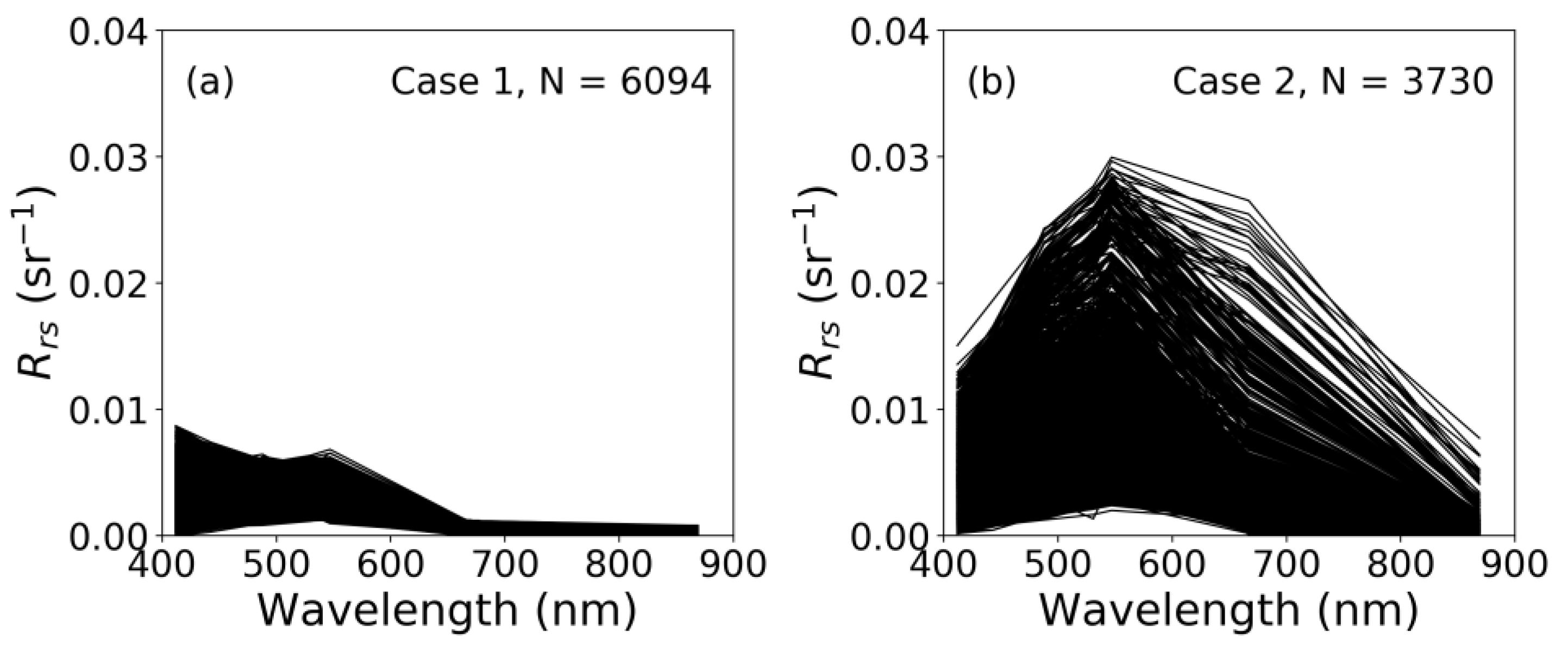
Such a relationship was used as input to the bio-optical model of Morel and Maritorena [13] to generate the threshold water irradiance reflectance just beneath the water surface, Rw(560), as a function of [Chla]. The effect of solar zenith angle was taken into consideration. For a given [Chla], if the observed Rw(560) exceeded the threshold Rw(560), the water was determined as Case 2, otherwise as Case 1. Note that the threshold of Morel and Bélanger [36] only distinguishes Case 2 turbid water with excessive sediments and detritus and does not separate yellow substance-dominated Case 2 waters. Therefore, the determined Case 1 water situations still included yellow substance-dominated Case 2 water situations. An additional threshold of remote sensing reflectance at 670 nm, i.e., Rrs(670) >0.0012 sr-1, now adopted as turbid water flag by the NASA Ocean Biology Processing Group (starting with the fourth processing), was also applied [37]. This second threshold may still not favor the identification of CDOM-dominated waters. With these two criteria, there are a total of 55 spectra classified as Case 1 and 445 spectra as Case 2 (Figure 1). Statistics including number of points (N), bias, root-mean-squared error (RMSE), and coefficient of determination (R2) were used to evaluate the model performance.
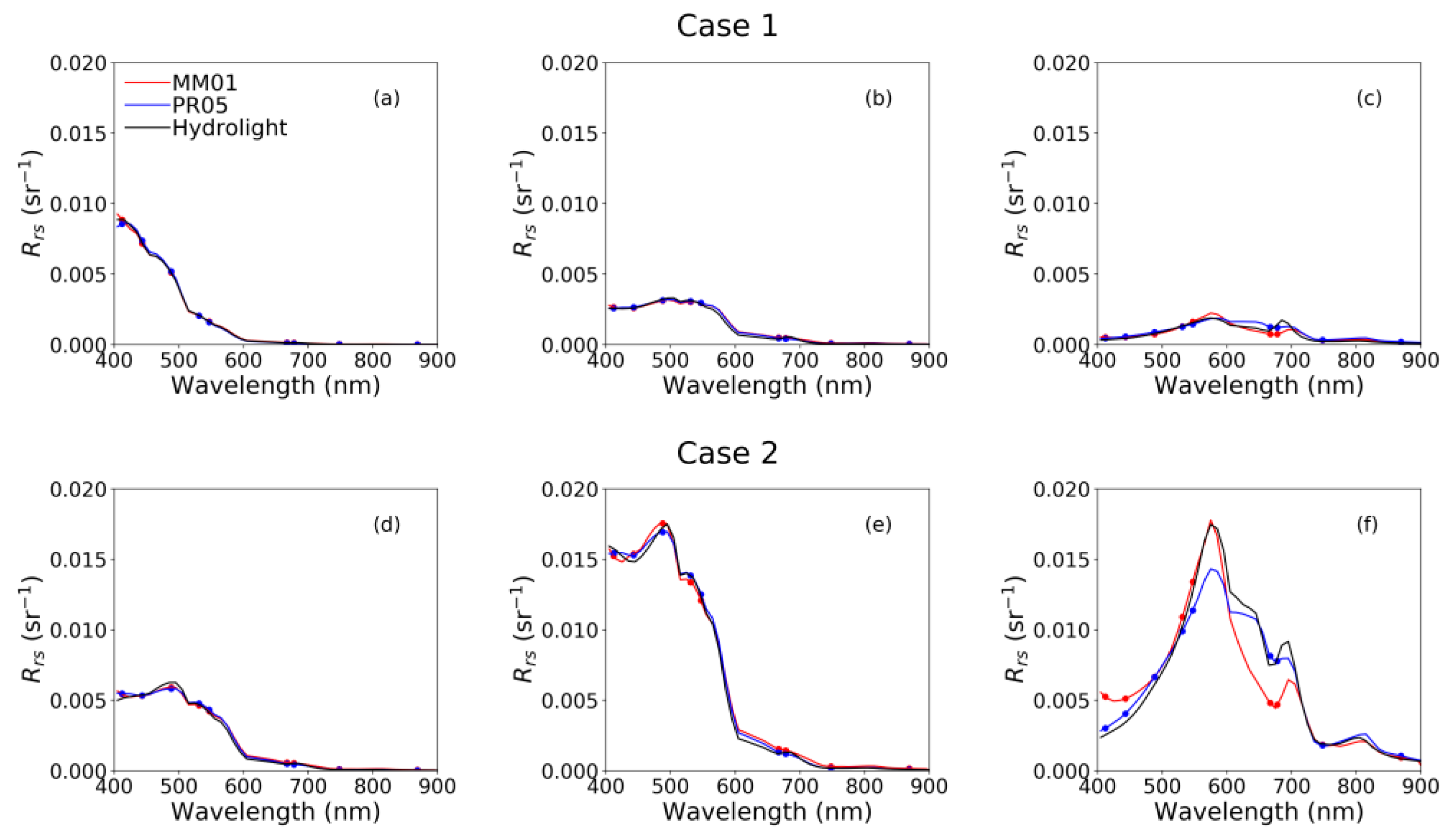
Figure 2 shows some examples of Rrs spectra reconstructed using the MM01 and PR05 models. Only 2 variable parameters, i.e., [Chla] and fb, are used in PR05, with fa fixed to 1. The MM01 and PR05 spectra generally agree with the Hydrolight simulated spectra, especially for Case 1 water (Figure 2a–c). As [Chla] is increased (Figure 2b,c), the difference between reconstructed and simulated Rrs around 680–700 nm becomes larger. This is expected since chlorophyll fluorescence effects are not considered in both models. The ability of the model to reproduce properly Rrs is degraded for Case 2 water (Figure 2d–f). In the complex Case 2 situation of Figure 2f, one noticeable feature of the MM01 reconstructed Rrs is the large discrepancy at 400–500 nm and 600–650 nm, which is attributed to neglecting CDOM absorption and crudely parameterizing the backscattering by non-algal particles. The disagreement around 550–650 nm between PR05 reconstructed and Hydrolight simulated Rrs is due to the fact that the slope of CDOM absorption adopted in the PR05 model, modeled as a function of [Chla], does not reflect well the actual (i.e., prescribed) slope, which ultimately affects the red wavelengths since the spectral-matching scheme minimizes the overall difference.
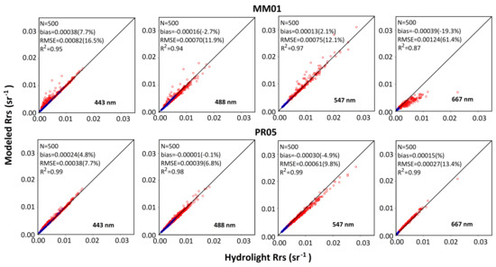
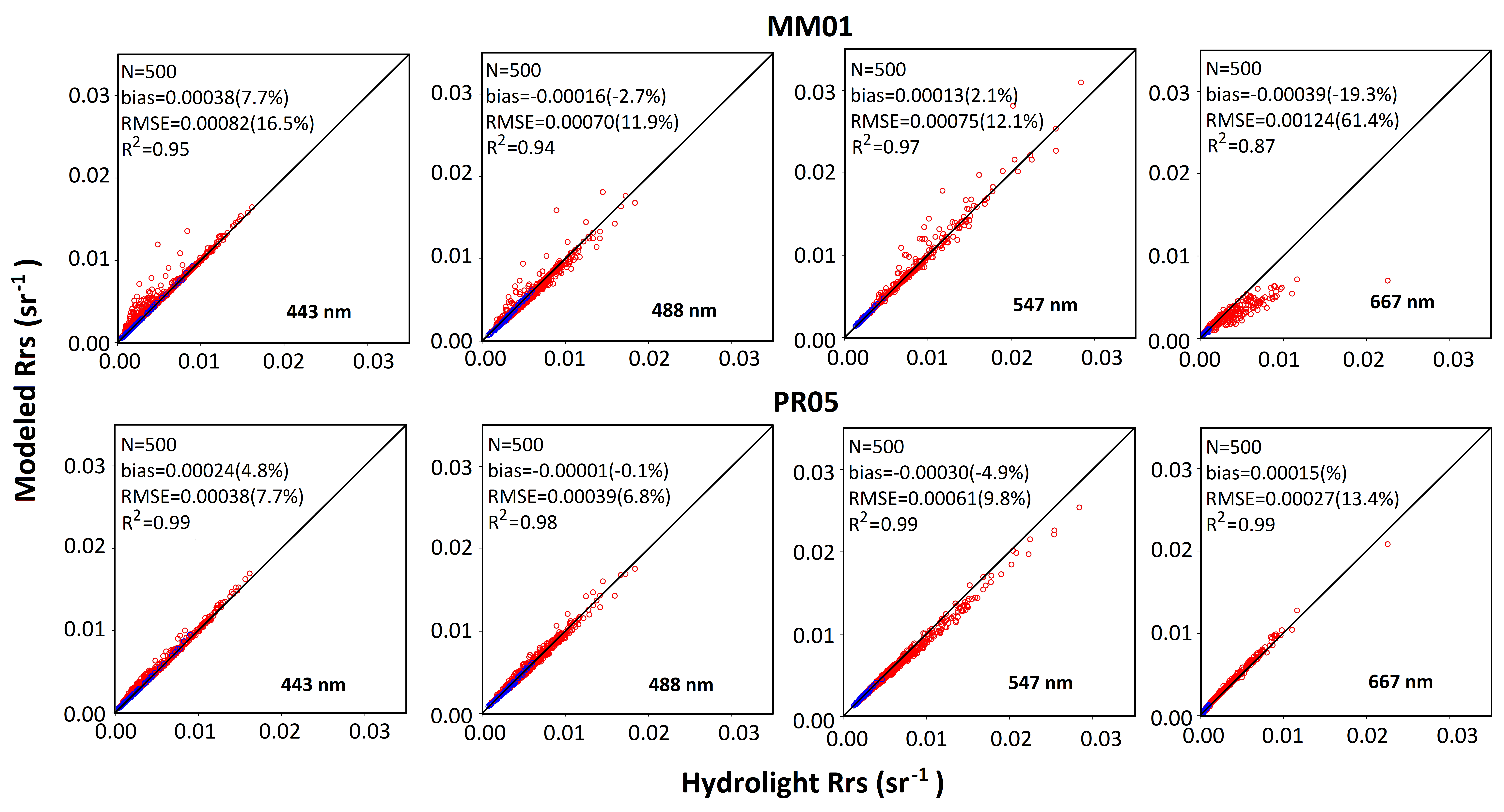
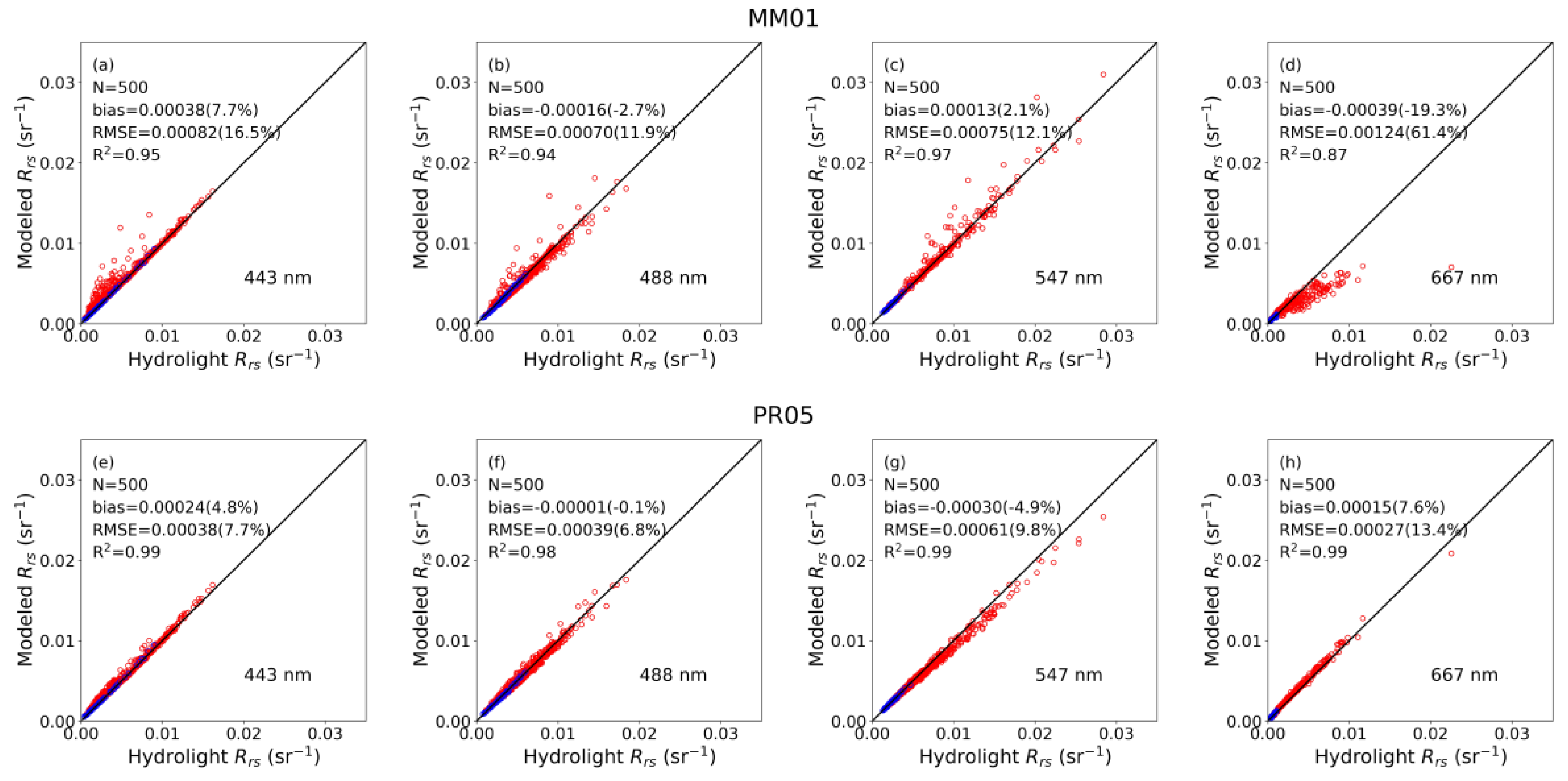
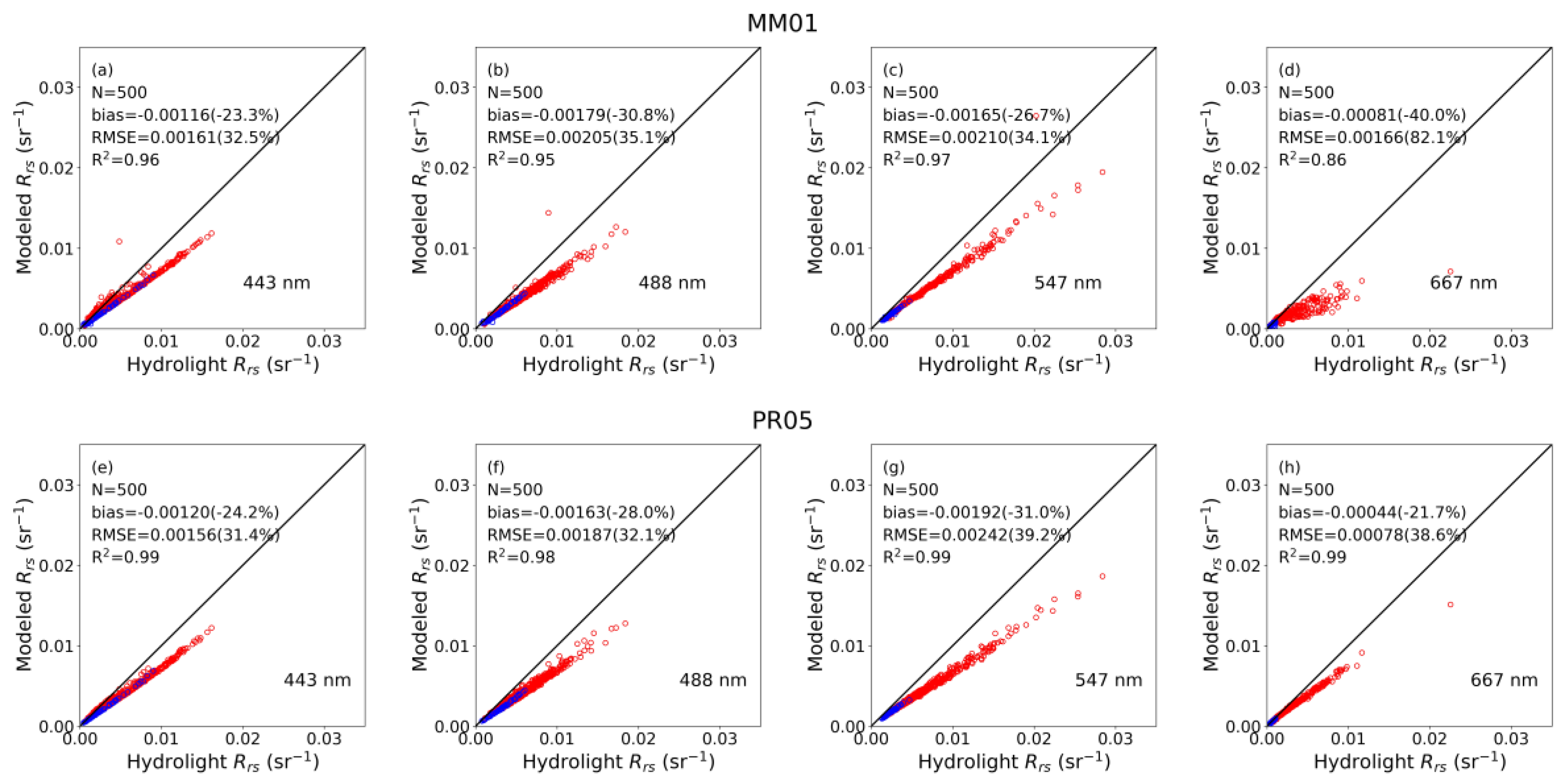
Figure 3 displays scatter plots of MM01 and PR05 reconstructed Rrs versus Hydrolight simulated Rrs at selected wavelengths, i.e., 443, 488, 547, and 667 nm, for all cases. The MM01 model performs generally well in reproducing Rrs at 443, 488, and 547 nm, with the performance for Case 1 water (Figure 3, blue) being better than that for Case 2 water (Figure 3, red), with overall bias and Root-Mean-Squared Error (RMSE) of 0.00038 (7.7%) and 0.00082 sr−1 (16.5%) at 443 nm, −0.00016 (−2.7%) and 0.00070 sr−1 (11.9%) at 488 nm, 0.00013 (2.1%) and 0.00075 sr−1 (12.1%) at 547 nm, and −0.00039 (−19.3) and 0.00124 sr−1 (61.4%) at 667 nm, respectively. The percent values in parentheses are biases or RMSEs normalized by the mean of the simulated data. The relatively high bias and RMSE for Case 2 water at 443 nm is due to the lack of CDOM absorption in the MM01 model and is consistent with Figure 2. The MM01 model performance is degraded at 667 nm. At this wavelength, large bias and RMSE are found for Case 2 water, although the reconstruction of Rrs is still good for Case 1 water. The degradation at 667 nm is due primarily to the backscattering of non-algal particles, not being sufficiently well treated by introducing bbs, and secondarily to fluorescence and CDOM absorption not considered. Since the spectral-matching scheme utilizes information at all the input wavelengths, neglecting CDOM absorption, influential in the blue, may also impact results in the red. The PR05 model shows better performance than the MM01 model in reconstructing Rrs at 443, 488, 547, and 667 nm, with bias and RMSE generally reduced, i.e., 0.00024 (4.8%) and 0.00038 sr−1 (7.7%) at 443 nm, −0.00001 (−0.1%) and 0.00039 sr−1 (6.8%) at 488 nm, −0.00030 (−4.9%) and 0.00061 sr−1 (9.8%) at 547 nm, and 0.00015 (7.6%) and 0.00027 sr−1 (13.4%) at 667 nm, respectively. The relatively large bias and RMSE at 547 nm, as compared to 443 and 488 nm, is due to the CDOM absorption slope, which is not adequately represented, as well as the spectral-matching scheme that minimizes the overall difference. The reconstructed Rrs at 667 nm is in good agreement with the Hydrolight values, which is consistent with the results shown in Figure 2. The improvement is dramatic at this wavelength when using PR05 instead of MM01 (e.g., RMSE reduced from 61.4% to 13.4%).
Performance statistics were computed separately for Case 1 and Case 2 water situations at all MODIS wavelengths (Table 1). The model results generally agree with the Hydrolight values, even in optically complex waters, with PR05 outperforming MM01 in almost all situations. Based on Table 1, the MM01 model generates Rrs more accurately for Case 1 water than for Case 2 water from 412 nm to 547 nm as the bias and RMSE values are lower, which is consistent with Figure 2 and Figure 3. The bias and RMSE for Case 1 water are less than 4.0% and 6.0%, respectively, while the bias can increase to 17.0% and the RMSE to 26.1% for Case 2 water. As wavelength becomes longer, i.e., from 667 nm to 869 nm, the bias and RMSE error increase for both Case 1 and Case 2 water situations. The reconstruction of Rrs at near infrared wavelengths, i.e., 748 and 869 nm, show large bias and RMSE (up to 45.6% and 78.3%, respectively). This is due mostly to the simplified treatment of non-algal particles via the addition of a backscattering coefficient with spectral dependence in λ−1 (and no absorption). Extending Rrs from 700 to 900 nm using the average similarity spectrum for turbid waters may also introduce errors. Similarly, the PR05 model generates more accurate Rrs estimation for Case 1 water than for Case 2 water from 412 nm to 547 nm. At these wavelengths, the largest bias observed is 2.1% and the largest RMSE 4.8% for Case 1 water, and the bias and RMSE increase up to 5.2% and 9.7%, respectively, for Case 2 water. The bias and RMSE errors increase (up to 13.7% and 22.2%, respectively) at 667 and 678 nm, indicating significant degradation in Rrs reconstruction at these wavelengths. Much larger relative errors are observed at the near infrared wavelengths, for both Case 1 and Case 2 situations, i.e., an RMSE of 47.3 and 21.7%, respectively, at 748 nm and 102.0 and 72.6%, respectively, at 869 nm, which reflects the generally lower Rrs, especially at 869 nm. This could also be partly due to the fact that the input absorption and scattering coefficients at these wavelengths are extrapolated values based on the values at 700 nm instead of based on field measurements. Compared with the POLYMER performance against in situ data obtained for the Medium Resolution Imaging Spectroradiometer (MERIS) in Case 1 water (Müller et al. [14]), the error in reconstructing Rrs from MM01 or PR05 (Table 1) is much smaller than the algorithm error, with RMSE values of 0.00008 (MM01) and 0.00012 (PR05) instead of 0.0011 sr−1 at 443 nm, and 0.00008 (MM01) and 0.00008 (PR05) at 547 nm instead of 0.00032 sr−1 at 560 nm. When data collected in both Case 1 and 2 waters are considered [14,38], the POLYMER RMSE values for MERIS are increased to 0.0037 sr−1 and 0.0033 sr−1 at 443 and 560 nm, respectively, which is much larger than the Rrs reconstruction errors, i.e., 0.00082 and 0.00038 at 443 nm and 547, respectively (Table 1). For MODIS-Aqua, these authors reported similar POLYMER performance, i.e., RMSE of 0.0036 at 443 nm and 0.0031 sr−1 at 547 nm. Thus, the error introduced by the semi-analytical modeling of water reflectance is unlikely to dominate the POLYMER performance, indicating that using MM01 and, especially, PR05 in the spectral-matching algorithm is adequate.
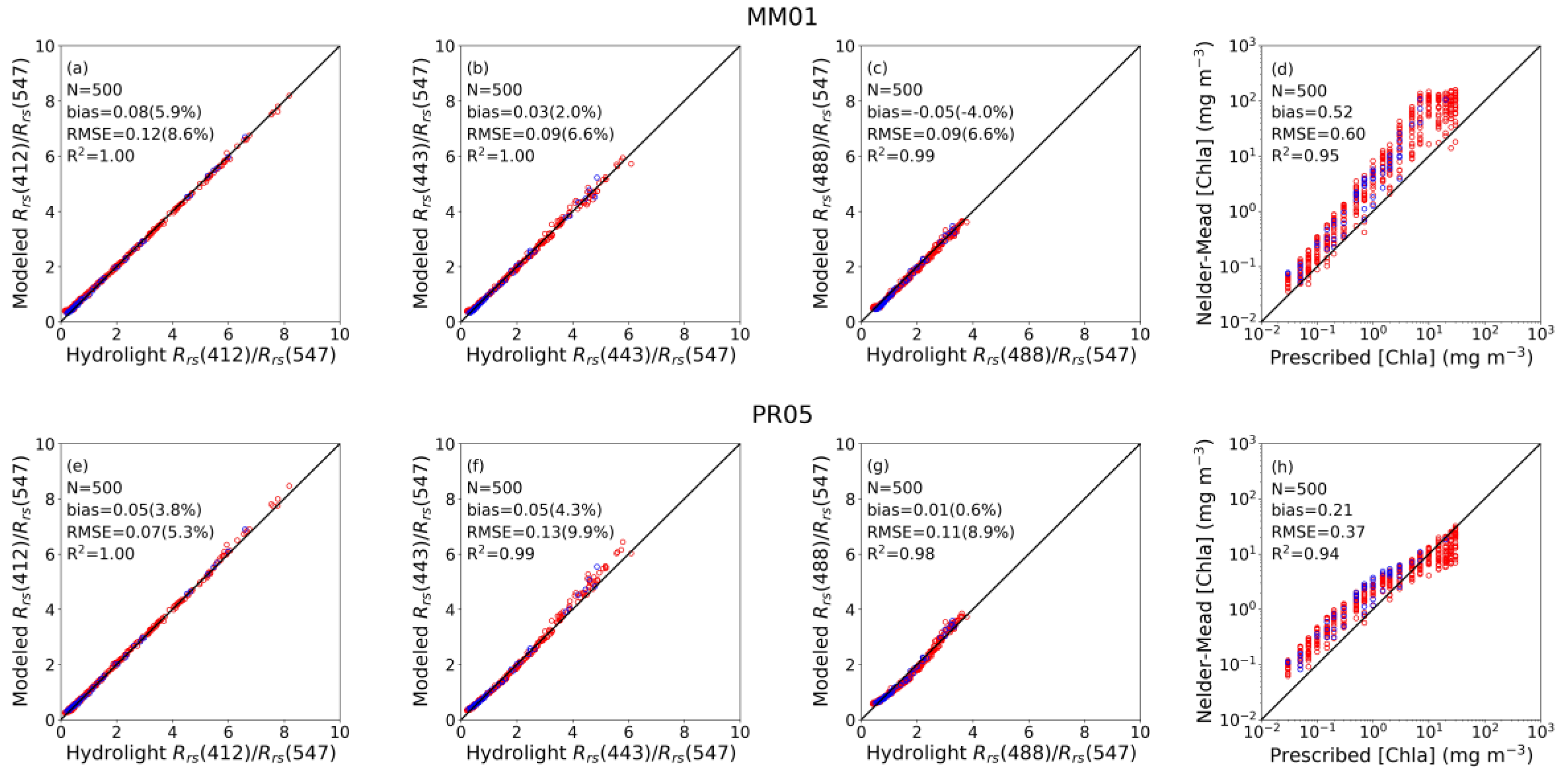
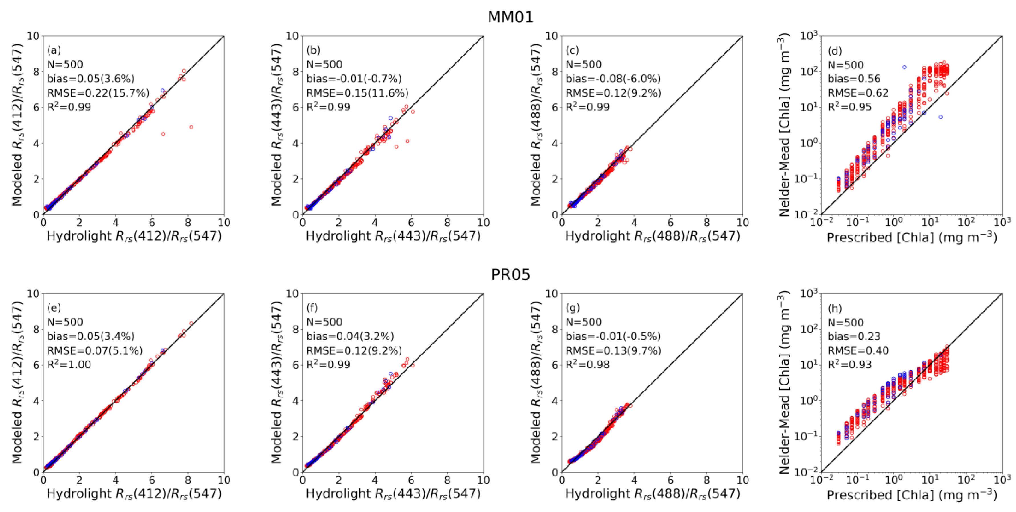
Figure 4 displays scatter plots of the model reconstructed and Hydrolight simulated Rrs ratios. Three ratios commonly used in ocean color algorithms [39,40] were selected, i.e., Rrs(412)/Rrs(547), Rrs(443)/Rrs(547), and Rrs(488)/Rrs(547). It is found that the MM01 and PR05 modeled band ratios Rrs(412)/Rrs(547), Rrs(443)/Rrs(547), and Rrs(488)/Rrs(547) are all in very good agreement with the Hydrolight simulations. The overall statistics indicate that the two models perform similarly in restituting Rrs ratios: the bias is less than 6% and the RMSE less than 9% for the MM01 model, and the bias is less than 5% and the RMSE less than 10% for the PR05 model. Also, the performance of Case 1 water situations is similar to that of Case 2 water situations (Table 2). This indicates that both the MM01 and PR05 models are capable of provide accurate estimation of Rrs ratios, which is important for ocean-color products using band ratio algorithms. If the MM01 and PR05 reconstructed Rrs is used in the OCI algorithm [41], the resulted bias and RMSE for estimated [Chla] are −0.000 (−0.2%) and 0.006 mgm−3 (4.3%), and −0.001 (−0.7%) and 0.008 mgm−3 (6.6%), respectively, i.e., much less than the errors caused by the OCI algorithm itself. This is due to the fact that the errors on Rrs at the various wavelengths considered in the CI equation, i.e., CI ≈ Rrs(555) − 0.5(Rrs(443) + Rrs(667)) where Rrs(555) is specified as 0.93Rrs(547) [41], are small (on the order of 10−4 sr−1) in the applicability domain of the algorithm (clear, Case 1 waters). Note for both models the Nelder–Mead retrieved [Chla] differs substantially from the prescribed [Chla] (Figure 4). The bias and RMSE of log10([Chla]) are 0.52 and 0.60, and 0.21 and 0.37, respectively, for MM01 and PR05 model, and the errors are similar for both Case 1 and Case 2 waters (Table 2). These values, especially biases, are much larger when compared with the MODIS-Aqua estimated [Chla] performance against in situ data which shows absolute bias and mean absolute error (MAE, always less or equal to RMSE) of 0.07 and 0.22 on log10 scale, respectively [42]. This is probably due to the variations in the relation between the absorption/ backscattering coefficients and the model parameters, which are not accounted for in the models. It is thus concluded that the [Chla] parameter in the models does not represent well the actual [Chla] and should not be used as [Chla] estimate. Instead [Chla] should be derived from the reconstructed Rrs, and using Rrs in band-ratio or OCI algorithms is appropriate.
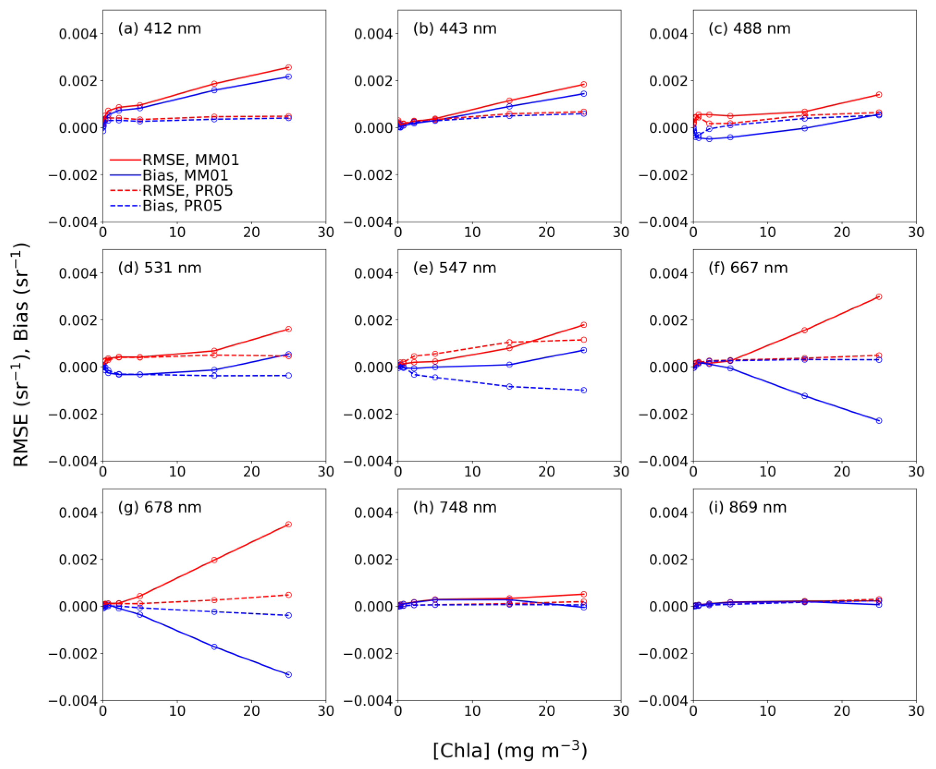
As seen in Figure 5, the errors generally increase when [Chla] increases for both MM01 and PR05 models. The bias and RMSE obtained for the PR05 model are generally lower than those for the MM01 model through the entire [Chla] range, confirming that the PR05 model provides better reconstruction of Rrs than the MM01 model. Specifically, the large bias and RMSE of the MM01 model, noticeably at 412 nm, 667 nm and 678 nm, are mainly related to the simplified treatment of backscattering of non-algal particles, as well as lack of fluorescence and absorption of CDOM and non-algal particles in the model. The large bias and RMSE at 547 nm of the PR05 model is due to the non-representative CDOM absorption slope, as discussed previously. The results also suggest degraded performance for Case 2 waters since these waters have generally higher [Chla] than Case 1 waters (bias and RMSE are larger for productive waters).
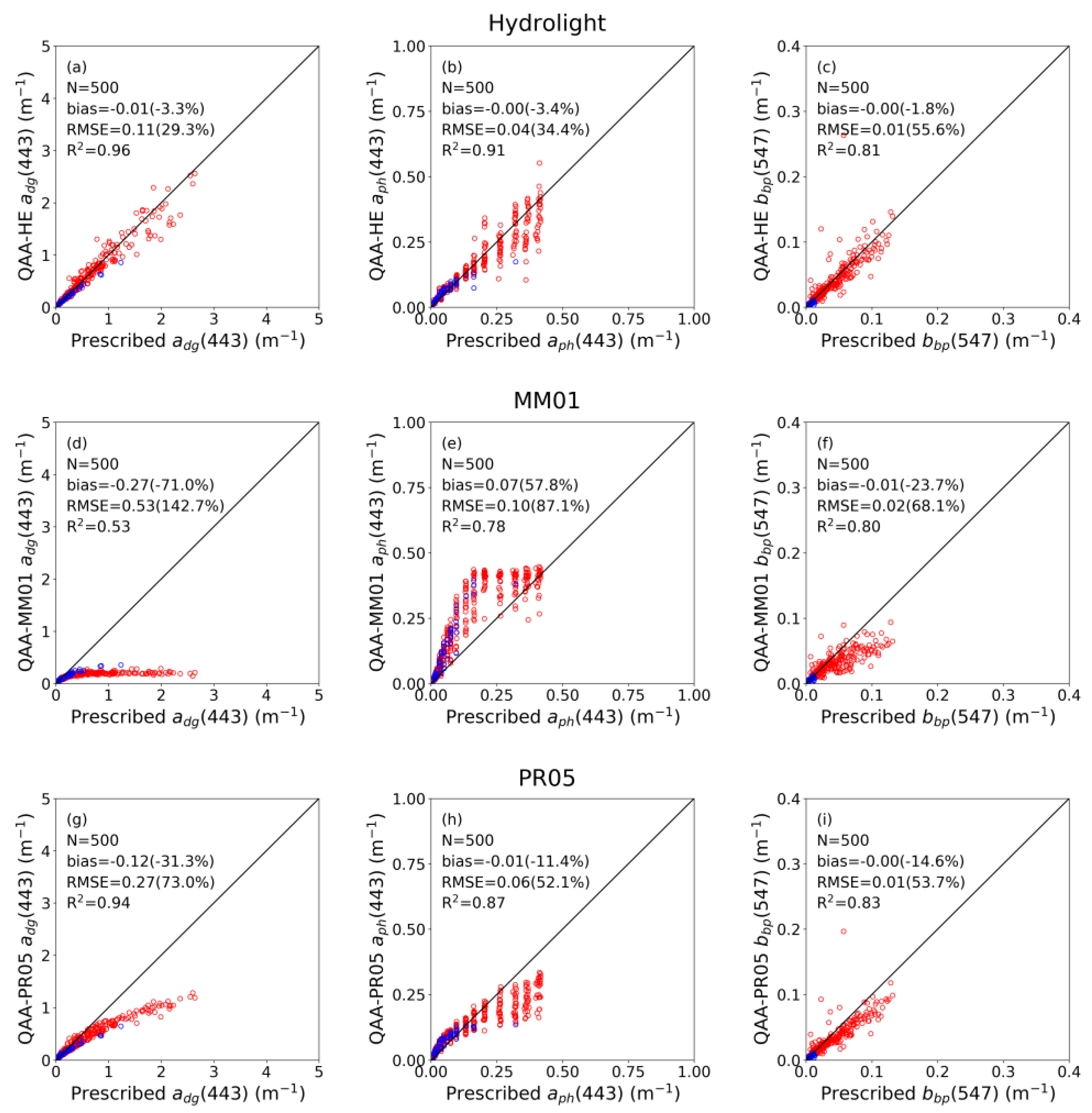
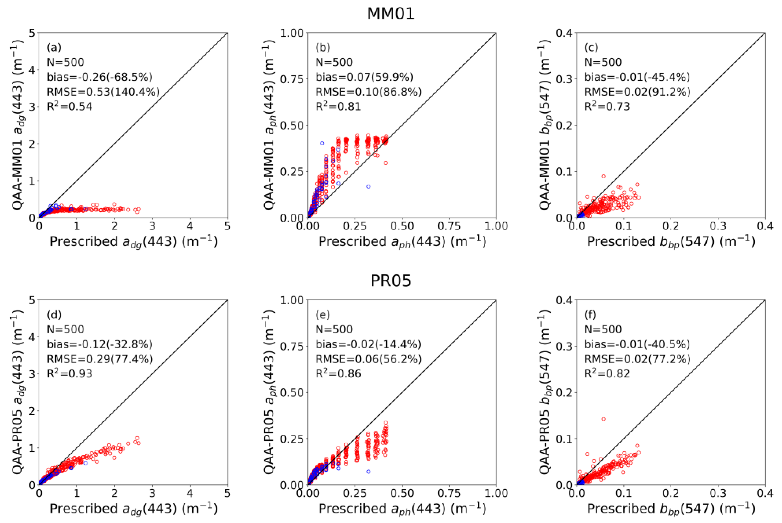
The MM01 and PR05 reconstructed Rrs were also used as input to the QAA algorithm [20] to retrieve IOPs including absorption of detritus and CDOM at 443 nm (adg(443)), phytoplankton absorption at 443 nm (aph(443)), and backscattering of particles at 547 nm (bbp(547)). When using the Hydrolight simulated Rrs as input to the QAA, the bias and RMSE for retrieved adg(443), aph(443), and bbp(547) are −3.3% and 29.3%, −3.4% and 34.4%, and −1.8% and 55.6%, respectively (Figure 6a–c). These values quantify algorithm errors. When using the reconstructed Rrs as input, the retrieved adg(443), aph(443), and bbp(443) are largely biased, i.e., bias being −71.0%, 57.8%, and −23.7% for MM01, and −31.3%, −11.4%, and −14.6% for PR05, when compared with the prescribed values (Figure 6d–i). The errors of using the MM01 and PR05 reconstructed Rrs are much higher than those of using Hydrolight simulated Rrs. Specifically, the performance of using the PR05 reconstructed Rrs is better than that of using the MM01 reconstructed Rrs with relatively lower bias and RMSE. The QAA algorithm involves two important parameters: u and χ, the first one depending on Rrs values and the second one depending on Rrs ratios. The value of bbp(547) depends on u at 547 nm, u(547), and the total absorption coefficient at 547 nm, a(547). Since u(547) is related to Rrs(547) only and a(547) is related to the ratio Rrs(443)/Rrs(547), Rrs(488)/Rrs(547), and Rrs(667)/Rrs(547), it is expected that the retrieved bbp(547) values show larger bias and RMSE compared with the retrieval using the Hydrolight simulated Rrs, and the errors are larger for the MM01 model than for the PR05 model based on the model performance in reconstructing Rrs(667) (Figure 3). The value of adg(443) is expressed as a function of bbp(547), Rrs(412), Rrs(443), and Rrs(443)/Rrs(547). Therefore, the error in the bbp(547) propagates further and results in much larger error in the retrieved adg(443), as shown in Figure 6d,g. Also, the retrieval error in adg(443) is less when using the PR05 model reconstructed Rrs due to the smaller error in bbp(547). The value of aph(443) is calculated as the total absorption minus adg and the absorption of pure sea water, in which way the error in retrieving aph(443) is compensated to some extent as the total absorption is derived using bbp(547) and Rrs(443). It is concluded that using successfully the QAA algorithm requires accurate input of Rrs and Rrs ratios. Other IOP algorithms such as GSM [43] and GIOP [44] also use Rrs as input and may have similar problems. Therefore, the MM01 and PR05 reconstructed Rrs should be used with caution to retrieve IOPs. One may envision, however, applying these inversion schemes to reflectance ratios, as long as sensitivity to IOPs remains adequate.
The three-parameter PR05 model was evaluated to figure out whether the Rrs reconstruction would be improved by introducing more parameters (Table 3). Results show that by introducing the third parameter fa (see Section 2.1), the PR05 model does improve the estimation of Rrs at all wavelengths except 531 nm, wavelength for which the bias and RMSE are slightly higher than using a two-parameter model. However, the improvement is not significant for 412, 443, 488, 547, and 667 nm, with bias and RMSE reduced by about 1% or even less. Much more improvement is seen at longer wavelengths (i.e., 678, 748, and 869 nm), but the differences between Hydrolight simulated and PR05 modeled Rrs are still large, for example the RMSE at 869 nm is 0.00010 sr−1 (56.1%). Similar results of Rrs are observed when separating Case 1 and Case 2 waters. Therefore, having a more intricate model may not be warranted. The trade-off is between efficiency/robustness and accuracy. It also should be noted that having more input parameters in the spectral-matching scheme might not guarantee convergence. It is concluded that the PR05 model with two parameters is preferred for Rrs estimation than the three-parameter model (allows faster and easier convergence while keeping similar accuracy).
3.2. Sensivity of Rrs Reconstruction to Atmospheric Transmittance
In the POLYMER algorithm, the TOA reflectance is decomposed as follows [13]:
where toz(λ) is the ozone transmittance, ρmol(λ) is the Rayleigh scattering reflectance, ρgli(λ) is the (non-spectral) sun glint reflectance affected by the direct transmission factor T(λ), ρaer(λ) is the aerosol reflectance, ρgam(λ) accounts for the coupling between Fresnel reflectance and scattering by molecules and aerosols, t(λ) is the total (i.e., direct + diffuse) transmittance for atmospheric scattering, and ρw(λ,0+) is the water reflectance above the water-air interface (ρw = πRrs). In this decomposition, the atmosphere is assumed to be clear (i.e., no clouds). In the presence of clouds, Equation (2) should be modified to account for scattering by cloud droplets and its interaction with molecule/aerosol scattering and surface reflection, and t(λ) should include cloud transmittance, i.e., t(λ) = tmol(λ) taer(λ) tcloud(λ), where subscripts mol, aer, and cloud refer to molecules, aerosols, and clouds, The transmittance t(λ) is pre-calculated with a successive orders of scattering (SOS) code [45] and stored in look-up tables, but only molecules are considered in the calculations, even though the algorithm is designed to work in the presence of aerosols and, at least, optically thin clouds. Neglecting the transmittance of aerosols and clouds is expected to affect the Rrs reconstruction in the spectral-matching scheme. Therefore, it is important to evaluate the sensitivity of the Rrs reconstruction using the MM01 and PR05 models to cloud and aerosol transmittance.
ρTOA(λ) = toz(λ)[ρmol(λ) + T(λ)ρgli(λ) + ρaer(λ) + ρgam(λ) + t(λ)ρw(λ,0+)]
To perform such evaluation, the aerosol total transmittance taer was modeled following Tanre et al. [46]:
where θs and θv are the Sun and view zenith angles, respectively, and τaer is the aerosol optical thickness, τaer(λ) = 0.1(λ/865)−1. The cloud transmittance tcloud was parameterized according to Fitzpatrick et al. [47]:
where τcloud is geometric-optics cloud optical thickness, α is surface albedo. Cloud optical depth τcloud is set to 3 (thin cloud), and surface albedo α to 0.06. Sun and view zenith angles are those of the IOCCG dataset, i.e., 30° and 0°, respectively. The coefficients a1, b1, b2, b3, k1, k2, k3, c, and d are tabulated in Fitzpatrick et al. [47] as a function of wavelength. The resulting tcloud values were interpolated to the MODIS wavelengths. With the calculated taer and tcloud, the Hydrolight simulated Rrs were transformed to Rrs taer tcloud, and the MM01 and PR05 model parameters were retrieved using Rrs taer tcloud instead of Rrs as input.
taer = exp[−0.16τaer(λ)(1/cos(θv) +1/cos(θs))],
tcloud = [a(τ) + b(τcloud) cosθv][a(τ) + b(τcloud)cosθs]/[1 + (c − dα)τcloud]2,
a(τ) = a1 + (1 − a1)exp(−k1τcloud),
b(τ) = b1[1 + b2exp(−k2τcloud) + b3exp(−k3τcloud)],
Figure 7 and Figure 8 display the resulting scatter plots of MM01 and PR05 reconstructed Rrs, [Chla], and Rrs ratios versus the Hydrolight simulations. The reconstructed Rrs is systematically biased, i.e., by 20–40%, after taking into account the cloud and aerosol transmittance. However, the Rrs ratios are still in good agreement with the Hydrolight simulated ratios, i.e., they exhibit bias and RMSE comparable to those obtained without considering the effects of transmittance. When using the MM01 and PR05 reconstructed Rrs to estimate [Chla] with the OCI algorithm, the resulting bias and RMSE increase to 0.039 (32.5%) and 0.040 mgm-3 (33.1%), and 0.036 (29.9%) and 0.036 mgm-3 (30.5%), respectively. This is because the cloud and aerosol transmittances introduce a large bias, i.e., more than 20%, to Rrs, which is further propagated to the CI index. The cloud and aerosol transmittances do not have much effect on the model-retrieved [Chla]; statistics are similar to those in Figure 4. However, again for both models, the Nelder–Mead [Chla] does not represent well the actual values. Note that most of the impact on the Rrs reconstruction performance is due cloud transmittance (0.78 at 443 nm), as the aerosol transmittance (0.95 at 443 nm) is close to 1.
When using the reconstructed Rrs as input to the QAA algorithm to retrieve adg(443), aph(443), and bbp(547), large errors are obtained compared with the results using the Hydrolight simulated reflectance spectra (Figure 9). As discussed in Section 3.1, the retrieved value of bbp(547) is dependent on Rrs(547), Rrs(443)/Rrs(547), Rrs(488)/Rrs(547), and Rrs(667)/Rrs(547). Since the reconstructed Rrs(547) is systematically biased when the effects of aerosol/cloud transmittance are taken into account (Figure 7), and even though the values of Rrs(443)/Rrs(547), Rrs(488)/Rrs(547), and Rrs(667)/Rrs(547) (Figure 8) are similar to those with no transmittance, the error in the retrieved bbp(547) is increased (compare Figure 9 with Figure 6). However, since adg(443) and aph(443) are not only determined by bbp(547) but also by Rrs(412), Rrs(443), and Rrs(443)/Rrs(547), in the end the errors somewhat compensate, yielding bias and RMSE for adg(443) and aph(443) that are similar to those before accounting for aerosol/cloud transmittance. Again, the errors in the retrieved IOPs are less when using the PR05 model reconstructed Rrs, compared with the MM01 results.
3.3. Model Performance Using AERONET-OC Dataset
Model (MM01, PR05) performance was further evaluated using the AERONET-OC dataset. The AERONET-OC dataset does not include Rrs at all wavelengths, i.e., only Rrs at 412, 443, 488, 531, 547, 667, and 869 nm are available. To determine if missing Rrs at 678 and 748 nm affects the model performance, tests were made using the 500 Hydrolight simulated cases (Section 2.3) with full MODIS wavelengths and with partial MODIS wavelengths (excluding 678 and 748 nm). No significant difference (i.e., less than 1%) in bias and RMSE was observed between Rrs, [Chla], and Rrs ratios retrieved using the full or partial set of wavelengths. Therefore, the errors caused by missing wavelengths are regarded as negligible in the following study. Prior to evaluation, Case 1 and Case 2 water situations were separated by using the same criteria that were applied to the Hydrolight simulations, taking the solar zenith angle into account. This resulted in 6094 Case 1 water and 3730 Case 2 water situations (Figure 10).
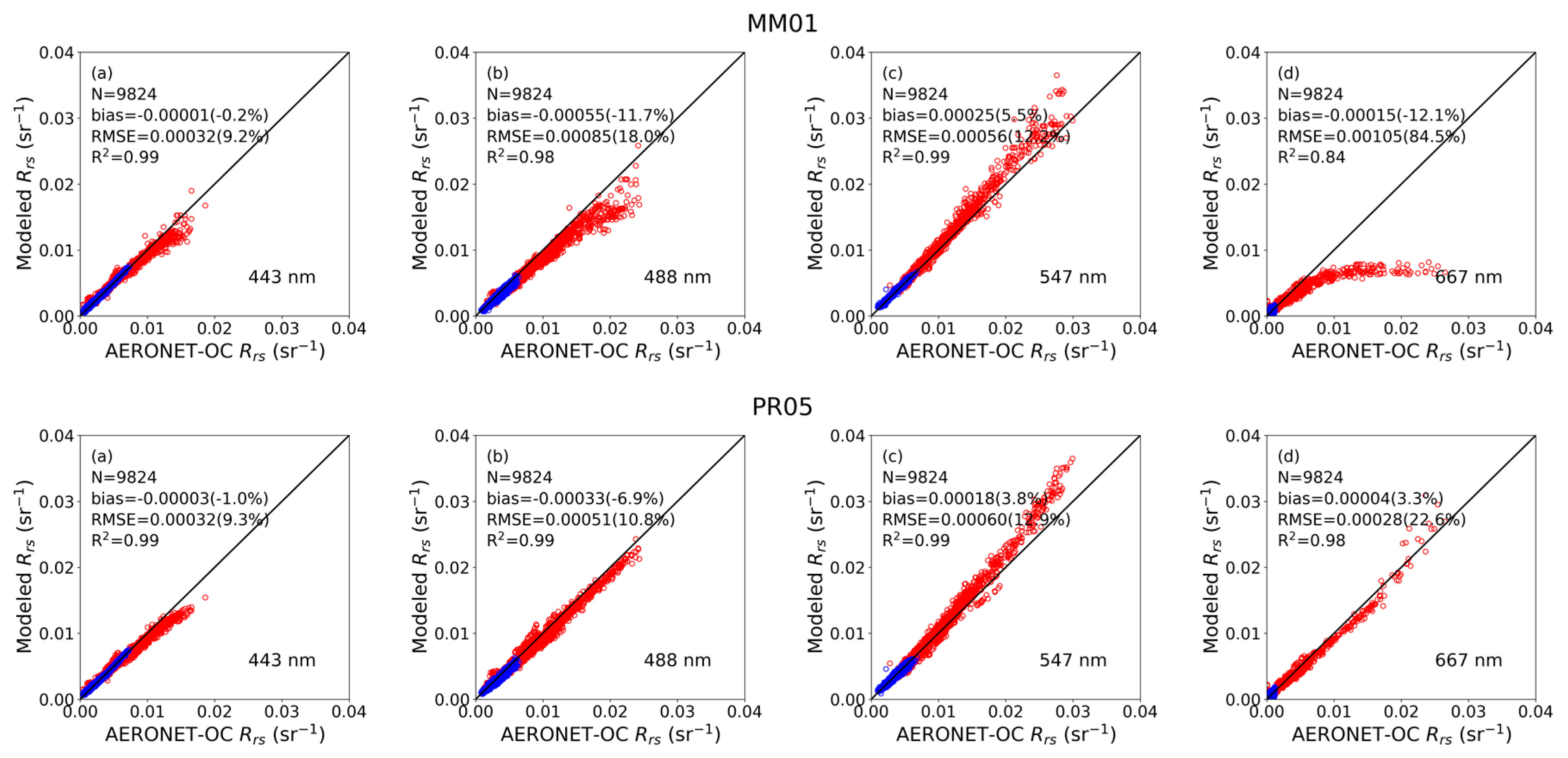
As shown in Figure 11, top and Table 4, the MM01 model performs generally well in reconstructing Rrs at 443, 488, and 547 nm. The bias and RMSE values are −0.00001 (−0.2%) and 0.00032 sr−1 (9.2%), −0.00055 (−11.7%) and 0.00085 sr−1 (18.0%), 0.00025 (5.5%) and 0.00056 sr−1 (12.2%) respectively, i.e., higher than those obtained using Hydrolight simulations. Much larger bias and RMSE are found at 667 nm, which are −0.00015 (−12.1%) and 0.0010 sr−1 (84.5%), respectively. Nevertheless, the errors in Rrs are still smaller than typical POLYMER atmospheric correction errors. The PR05 model performs better in reconstructing Rrs with generally lower bias and RMSE at each wavelength (Figure 11, bottom, and Table 4). Unlike for the MM01 model, the PR05 reconstructed Rrs values at 667 nm are in good agreement with the AERONET-OC measurements, even though fluorescence is not considered in the PR05 model. Similar to the MM01 results, the bias and RMSE values of the PR05 reconstruction are higher than those obtained using Hydrolight simulations. As discussed in the previous section, the simplified representation of the backscattering of non-algal particles, together with the lack of consideration of fluorescence and CDOM and non-algal absorption in the MM01 model are the main contributors to the errors in reconstructed Rrs. The PR05 model takes into account the absorption and backscattering of non-algal particles by using the [Chla] and fb parameters, but the slope used for CDOM absorption might not be sufficiently well representative, causing substantial errors at 547 nm for Case 2 water situations when applying the spectral-matching scheme for inversion. Note that the Hydrolight simulated Rrs is not subjected to radiometric errors and other, e.g., environmental, perturbations and this may partly explain why the bias and RMSE in reconstructed Rrs using the AERONET-OC dataset are larger than those obtained using Hydrolight simulations.
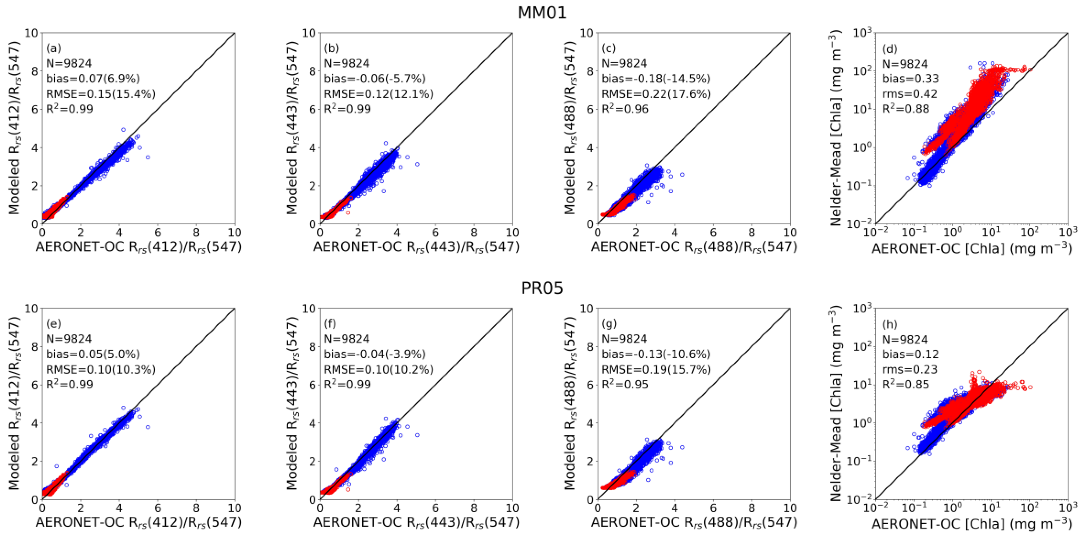
Figure 12 displays scatter plots of the model reconstructed and AERONET-OC measured Rrs ratios. Results show that the MM01 and PR05 band ratios Rrs(412)/Rrs(547), Rrs(443)/Rrs(547), and Rrs(488)/ Rrs(547) are all in good agreement with the AERONET-OC measurements. The overall bias is less than 15% and the overall RMSE less than 18% for the MM01 model. The PR05 reconstruction gives slightly better results, with the overall bias less than 11% and the overall RMSE less than 16%. As expected, the errors in the reconstructed Rrs ratios are larger than those obtained using Hydrolight simulations. Table 5 shows that the model reconstructed Rrs ratios agree well with the prescribed values for both Case 1 and Case 2 waters, with errors slightly lower for Case 1 situations than for Case 2 situations. When applying the MM01 and PR05 reconstructed Rrs to estimate [Chla] using the OCI algorithm, the resulting bias and RMSE for [Chla] are 0.010 (4.8%) and 0.014 mgm-3 (6.8%), and 0.007 (3.6%) and 0.011 mgm-3 (5.4%), respectively. This confirms that both the MM01 and PR05 reconstructed Rrs can be used to estimate [Chla] using band ratio and OCI algorithms. Figure 12 also shows that the model-retrieved [Chla] differs substantially from the AERONET-OC [Chla], both models tending to overestimate [Chla]. However, for both models the overall agreement is better than when using Hydrolight simulations: the bias and RMSE on log10 scale are 0.33 and 0.42 instead of 0.52 and 0.60, respectively, for the MM01 model, and 0.12 and 0.23 instead of 0.21 and 0.37, respectively, for the PR05 model. The statistics are similar when Case 1 and Case 2 waters are used separately (Table 5). The comparisons suggest that the bio-optical relationships used in both models, based on field measurements, are more representative of actual situations than those in the Hydrolight simulations. Despite the improvement in [Chla] estimate, the model-retrieved [Chla] should still not be considered as representative of the actual [Chla].
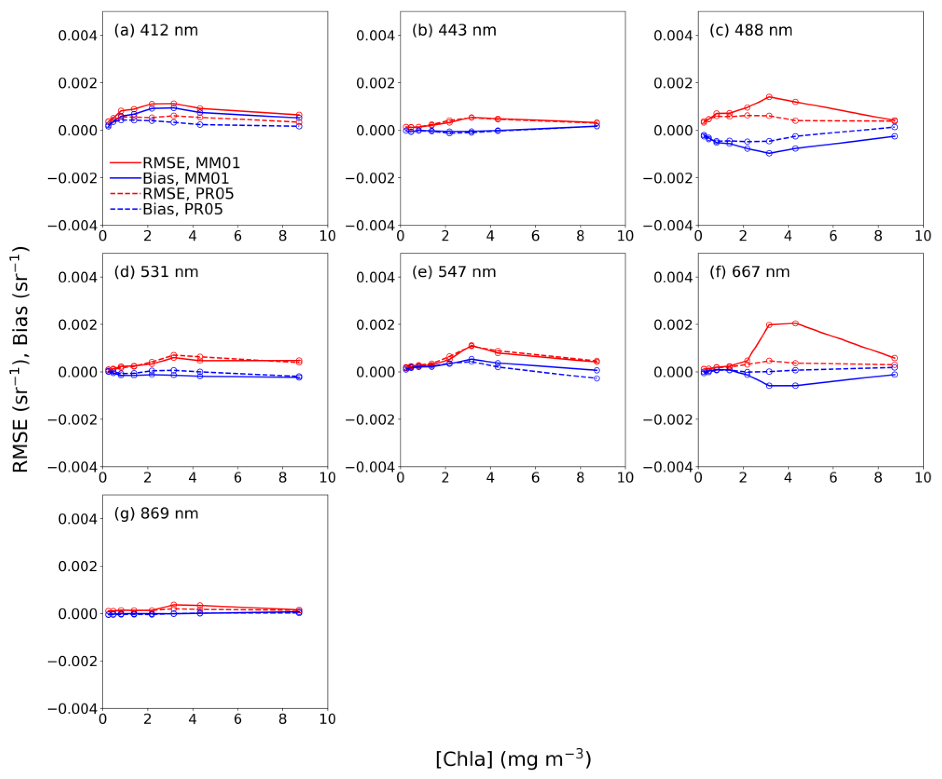
When using the MM01 model for Rrs reconstruction, relatively large bias and RMSE are observed at 488 nm (when [Chla] is within 2–4 mg m−3) and 667 nm (when [Chla] is larger than 2 mg m−3) (Figure 13). Such behavior could be due to the fact that the absorption and backscattering of non-algal particles, fluorescence, and CDOM absorption are not taken into account in the MM01 model. For other wavelengths the bias and RMSE are relatively small and do not quite change with [Chla], except when [Chla] is within 2–4 mg m−3 (small increase). This is also the case when using PR05 model. This increased bias and RMS when [Chla] is in the range 2–4 mg m−3 could be due to the fact that the AERONET-OC [Chla] are not measured but estimated from remote sensing reflectance [19], and that higher uncertainty exists in this [Chla] range. It is also possible the variability of chlorophyll-a absorption is not sufficiently well represented in the MM01 and PR05 model. The bias and RMSE are smaller over the entire [Chla] range when using the PR05 model, indicating the overall better performance of that model in reconstructing water reflectance, again confirming the results from simulations.
4. Summary and Conclusions
The MM01 and PR05 models used in the POLYMER spectral-matching algorithm have been examined in terms of their ability to properly represent water reflectance over the wide range of situations/regimes expected in oceans. The MM01 model, in the modified version considered, depends on chlorophyll-a concentration and backscattering coefficient for non-algal particles. The PR05 model depends on chlorophyll-a concentration, a parameter specifying the contribution of algal and non-algal particles to the backscattering coefficient, and a parameter allowing different absorption coefficients for dissolved organic matter. The two models have been evaluated separately for Case 1 and Case 2 waters at MODIS wavelengths (412, 443, 488, 531, 547, 667, 678, 748, and 869 nm).
A theoretical evaluation was first performed using Hydrolight simulations with IOPs from an IOCCG synthesized dataset (500 cases) representing a wide range of field observations. Results show that the MM01 model generally performs well in retrieving Rrs at 412, 443, 488, 531, and 547 nm, even in optically complex waters. Neglecting CDOM absorption in the MM01 model is responsible for the relatively large bias and RMS found at 412 nm. The discrepancies found at 667 and 869 nm for Case 2 water are mainly due to the backscattering of inorganic particles not well represented in the MM01 model. Other factors, including compensation by the spectral-matching scheme of differences at shorter wavelengths caused by the lack of CDOM and non-algal absorption and Rrs extrapolation above 700 nm using the similarity spectrum, may also contribute to degradation of performance at 667 and 869 nm. Despite the errors in Rrs, the MM01 retrieved Rrs ratios are in very good agreement with the Hydrolight Rrs ratios. The PR05 model, on the other hand, shows better performance than the MM01 model in reconstructing Rrs. The PR05 retrieved Rrs values, obtained by fixing to unity the parameter allowing variable absorption by dissolved organic matter, agree with the Hydrolight values for both Case 1 and Case 2 situations at all visible wavelengths including 667 and 678 nm, even though fluorescence is not considered in the model. The relatively large bias and RMSE at 547 nm is due to the non-representative slope of CDOM absorption and the spectral-matching scheme that minimizes the overall difference. Large discrepancy with the Hydrolight Rrs values is found at 748 and 869 nm, which reflects the generally lower Rrs, especially at 869 nm, and could be partly due to the fact that the input absorption and scattering coefficients at these wavelengths are extrapolated from values at 700 nm instead of based on field measurements. Overall, the performance for Case 1 waters is better than that of for Case 2 waters. The PR05 reconstructed Rrs ratios also agree well with the Hydrolight ratios. The reconstructed Rrs from both models, when used in the OCI algorithm for oligotrophic waters, yields an accurate estimation of chlorophyll-a concentration. However, the MM01 and PR05 retrieved Rrs, when used as input to the QAA algorithm, gives significant errors in the estimation of aph(443), adg(443), and bbp(547). This is due to the fact that the QAA algorithm uses Rrs at all visible wavelengths and not only Rrs ratios. Therefore, caution should be exercised when using the model-retrieved Rrs in algorithms for IOP estimations such as QAA. Importantly, the model parameters that best fit the input data, in particular chlorophyll-a concentration, may not represent adequately actual values. The impact of cloud and aerosol transmittance (assumed to be 1 in POLYMER) on Rrs reconstruction was also evaluated theoretically using Hydrolight simulations. While the cloud and aerosol transmittances do not affect significantly the reconstruction of Rrs ratios, they do affect the accuracy of reconstructed Rrs, the OCI estimated chlorophyll-a concentration, and the derived IOPs when using QAA and, presumably, other IOP algorithms.
The MM01 and PR05 models were further evaluated using the AERONET-OC dataset, which consists of 9824 samples from a total of 15 sites. Only Rrs measurements at 412, 443, 488, 531, 547, 667, and 869 nm were available, but the missing data at 678 and 748 nm does not affect significantly the Rrs retrievals as tested using the Hydrolight simulations. Similar conclusions to those obtained with simulated Rrs are drawn for the model-retrieved Rrs and Rrs ratios, confirming the theoretical results, but with relatively higher bias and RMSE probably due to the uncertainties existing in field measurements, and the IOP variability not captured by both models. In any case, the uncertainty in reconstructing Rrs is much smaller than typical POLYMER atmospheric correction errors obtained against in-situ measurements. Again, the model-retrieved chlorophyll-a concentration does not agree well with the AERONET-OC values, which may partly result from the application of non-site-specific bio-optical algorithms. Therefore, it is recommended that the reconstructed water reflectance, not the retrieved model parameters, should be used in bio-optical algorithms.
The three-parameter PR05 model was also evaluated using the Hydrolight simulations, to examine whether using more parameters would improve the reconstruction of the water reflectance. Reconstruction was improved with three parameters, but slightly. Using more parameters, however, increases computation time and is less likely to guarantee convergence of the spectral matching scheme. The trade-off is between efficiency/robustness and accuracy. It is concluded that the two-parameter PR05 model is preferred and appropriate to represent the reflectance of a wide range of Case 1 and case 2 waters in spectral-matching atmospheric correction schemes such as POLYMER, and probably other (e.g., statistical) one-step inversion schemes, at least until progress in atmospheric correction necessitates otherwise.
Author Contributions
Conceptualization, methodology and investigation: J.T. and R.F.; writing—original draft preparation: J.T.; writing—review and editing: R.F., D.R., F.S., and G.Z.; supervision: R.F.
Funding
The National Aeronautics and Space Administration (NASA) provided funding for this research under grants NNX14AM3G and NNX14AQ46A.
Acknowledgments
The authors wish to thank Zhongping Lee, University of Boston, for generating and making available the synthesized IOCCG data set, Giuseppe Zibordi, Joint Research Centre of the European Union, and the principal investigators, scientists, and technicians responsible for collecting, processing, and archiving the AERONET-OC data, and John McPherson, Scripps Institution of Oceanography, for technical help. Zibordi provided useful comments on the manuscript. The support of NASA’s Ocean Biology/ Biogeochemistry Program, managed by Paula Bontempi and Laura Lorenzoni, is gratefully acknowledged.
Conflicts of Interest
The authors declare no conflict of interest.
References
- Frouin, R.J.; Franz, B.A.; Ibrahim, A.; Knobelspiesse, K.; Ahmad, Z.; Cairns, B.; Chowdhary, J.; Dierssen, H.M.; Tan, J.; Dubovik, O.; et al. Atmospheric Correction of Satellite Ocean-Color Imagery During the PACE Era. Front. Earth Sci. 2019, 7, 145. [Google Scholar] [CrossRef]
- Chomko, R.M.; Gordon, H.R. Atmospheric correction of ocean color imagery: use of the Junge power-law aerosol size distribution with variable refractive index to handle aerosol absorption. Appl. Opt. 1998, 37, 5560. [Google Scholar] [CrossRef] [PubMed]
- Land, P.E.; Haigh, J.D. Atmospheric correction over case 2 waters with an iterative fitting algorithm: relative humidity effects. Appl. Opt. 1997, 36, 9448. [Google Scholar] [CrossRef] [PubMed]
- Stamnes, K.; Li, W.; Yan, B.; Eide, H.; Barnard, A.; Pegau, W.S.; Stamnes, J.J. Accurate and self-consistent ocean color algorithm: simultaneous retrieval of aerosol optical properties and chlorophyll concentrations. Appl. Opt. 2003, 42, 939. [Google Scholar] [CrossRef] [PubMed]
- Kuchinke, C.P.; Gordon, H.R.; Franz, B.A. Spectral optimization for constituent retrieval in Case 2 waters I: Implementation and performance. Remote Sens. Environ. 2009, 113, 571–587. [Google Scholar] [CrossRef]
- Shi, C.; Nakajima, T.; Hashimoto, M. Simultaneous retrieval of aerosol optical thickness and chlorophyll concentration from multiwavelength measurement over East China Sea. J. Geophys. Res.: Atmos. 2016, 121, 14084–14101. [Google Scholar] [CrossRef]
- Gordon, H.R. Removal of atmospheric effects from satellite imagery of the oceans. Appl. Opt. 1978, 17, 1631. [Google Scholar] [CrossRef]
- Sathyendranath, S.; Prieur, L.; Morel, A. A three-component model of ocean colour and its application to remote sensing of phytoplankton pigments in coastal waters. Int. J. Remote Sens. 1989, 10, 1373–1394. [Google Scholar] [CrossRef]
- D’Sa, E.J.; Miller, R.L.; Del Castillo, C. Bio-optical properties and ocean color algorithms for coastal waters influenced by the Mississippi River during a cold front. Appl. Opt. 2006, 45, 7410. [Google Scholar] [CrossRef]
- D’Sa, E.J.; DiMarco, S.F. Seasonal variability and controls on chromophoric dissolved organic matter in a large river-dominated coastal margin. Limnol. Oceanogr. 2009, 54, 2233–2242. [Google Scholar] [CrossRef]
- Komick, N.M.; Costa, M.P.F.; Gower, J. Bio-optical algorithm evaluation for MODIS for western Canada coastal waters: An exploratory approach using in situ reflectance. Remote Sens. Environ. 2009, 113, 794–804. [Google Scholar] [CrossRef]
- O’Donnell, D.M.; Effler, S.W.; Strait, C.M.; Leshkevich, G.A. Optical characterizations and pursuit of optical closure for the western basin of Lake Erie through in situ measurements. J. Great Lakes Res. 2010, 36, 736–746. [Google Scholar] [CrossRef]
- Steinmetz, F.; Deschamps, P.-Y.; Ramon, D. Atmospheric correction in presence of sun glint: application to MERIS. Opt. Express 2011, 19, 9783. [Google Scholar] [CrossRef] [PubMed]
- Müller, D.; Krasemann, H.; Brewin, R.J.W.; Brockmann, C.; Deschamps, P.-Y.; Doerffer, R.; Fomferra, N.; Franz, B.A.; Grant, M.G.; Groom, S.B.; et al. The Ocean Colour Climate Change Initiative: I. A methodology for assessing atmospheric correction processors based on in-situ measurements. Remote Sens. Environ. 2015, 162, 242–256. [Google Scholar]
- Müller, D.; Krasemann, H.; Brewin, R.J.W.; Brockmann, C.; Deschamps, P.-Y.; Doerffer, R.; Fomferra, N.; Franz, B.A.; Grant, M.G.; Groom, S.B.; et al. The Ocean Colour Climate Change Initiative: II. Spatial and temporal homogeneity of satellite data retrieval due to systematic effects in atmospheric correction processors. Remote Sens. Environ. 2015, 162, 257–270. [Google Scholar] [CrossRef]
- Morel, A.; Maritorena, S. Bio-optical properties of oceanic waters: A reappraisal. J. Geophys. Res.: Ocean. 2001, 106, 7163–7180. [Google Scholar] [CrossRef]
- Park, Y.-J.; Ruddick, K. Model of remote-sensing reflectance including bidirectional effects for case 1 and case 2 waters. Appl. Opt. 2005, 44, 1236. [Google Scholar] [CrossRef]
- IOCCG. Remote Sensing of Inherent Optical Properties: Fundamentals, Tests of Algorithms, and Applications; Reports of the International Ocean-Colour Coordinating Group, No. 5; Lee, Z.-P., Ed.; IOCCG: Dartmouth, NS, Canada, 2006. [Google Scholar]
- Zibordi, G.; Mélin, F.; Berthon, J.-F.; Holben, B.; Slutsker, I.; Giles, D.; D’Alimonte, D.; Vandemark, D.; Feng, H.; Schuster, G.; et al. AERONET-OC: A network for the validation of ocean color primary products. J. Atmos. Ocean. Technol. 2009, 26, 1634–1651. [Google Scholar] [CrossRef]
- Lee, Z.; Carder, K.L.; Arnone, R.A. Deriving inherent optical properties from water color: A multiband quasi-analytical algorithm for optically deep waters. Appl. Opt. 2002, 41, 5755. [Google Scholar] [CrossRef]
- Morel, A.; Gentili, B. Diffuse reflectance of oceanic waters III Implication of bidirectionality for the remote-sensing problem. Appl. Opt. 1996, 35, 4850. [Google Scholar] [CrossRef]
- Ruddick, K.G.; De Cauwer, V.; Park, Y.-J.; Moore, G. Seaborne measurements of near infrared water-leaving reflectance: The similarity spectrum for turbid waters. Limnol. Oceanogr. 2006, 51, 1167–1179. [Google Scholar] [CrossRef]
- Westberry, T.K.; Boss, E.; Lee, Z. Influence of Raman scattering on ocean color inversion models. Appl. Opt. 2013, 52, 5552. [Google Scholar] [CrossRef] [PubMed]
- Nelder, J.A.; Mead, R. A simplex method for function minimization. Comput. J. 1965, 7, 308–313. [Google Scholar] [CrossRef]
- Morel, A. Optical modeling of the upper ocean in relation to its biogenous matter content (case I waters). J. Geophys. Res. 1988, 93, 10749. [Google Scholar] [CrossRef]
- Pope, R.M.; Fry, E.S. Absorption spectrum (380–700 nm) of pure water II Integrating cavity measurements. Appl. Opt. 1997, 36, 8710. [Google Scholar] [CrossRef]
- Smith, R.C.; Baker, K.S. Optical properties of the clearest natural waters (200–800 nm). Appl. Opt. 1981, 20, 177. [Google Scholar] [CrossRef]
- Gregg, W.W.; Carder, K.L. A simple spectral solar irradiance model for cloudless maritime atmospheres. Limnol. Oceanogr. 1990, 35, 1657–1675. [Google Scholar] [CrossRef]
- Bricaud, A.; Babin, M.; Morel, A.; Claustre, H. Variability in the chlorophyll-specific absorption coefficients of natural phytoplankton: Analysis and parameterization. J. Geophys. Res. 1995, 100, 13321. [Google Scholar] [CrossRef]
- Bricaud, A.; Morel, A.; Babin, M.; Allali, K.; Claustre, H. Variations of light absorption by suspended particles with chlorophyll a concentration in oceanic (case 1) waters: Analysis and implications for bio-optical models. J. Geophys. Res.: Ocean. 1998, 103, 31033–31044. [Google Scholar] [CrossRef]
- Roesler, C.S.; Perry, M.J.; Carder, K.L. Modeling in situ phytoplankton absorption from total absorption spectra in productive inland marine waters. Limnol. Oceanogr. 1989, 34, 1510–1523. [Google Scholar] [CrossRef]
- Kirk, J.T.O. Light and Photosynthesis in Aquatic Ecosystems; Cambridge University Press: Cambridge, UK, 1994; ISBN 0521459664. [Google Scholar]
- Voss, K.J. A spectral model of the beam attenuation coefficient in the ocean and coastal areas. Limnol. Oceanogr. 1992, 37, 501–509. [Google Scholar] [CrossRef]
- Gordon, H.R.; Morel, A.Y. Remote Assessment of Ocean Color for Interpretation of Satellite Visible Imagery: A Review; Lecture Notes on Coastal and Estuarine Studies; American Geophysical Union: Washington, DC, USA, 1983; Volume 4, ISBN 0-387-90923-0. [Google Scholar]
- Loisel, H.; Morel, A. Light scattering and chlorophyll concentration in case 1 waters: A reexamination. Limnol. Oceanogr. 1998, 43, 847–858. [Google Scholar] [CrossRef] [Green Version]
- Morel, A.; Bélanger, S. Improved detection of turbid waters from ocean color sensors information. Remote Sens. Environ. 2006, 102, 237–249. [Google Scholar] [CrossRef]
- Robinson, W.D.; Franz, B.A.; Patt, F.S.; Bailey, S.W.; Werdell, P.J. Masks and flags updates. In SeaWiFS Postlauch Technical Report Series; NASA/TM-2003-206892; Hook, S.B., Firestone, E.R., Eds.; National Aeronautics and Space Administration, Goddard Space Flight Center: Greenbelt, MD, USA, 2003; Volume 22, pp. 34–40. [Google Scholar]
- Krasemann, H.; Müller, D. Ocean Colour Climate Change Initiative (OC-CCI)—Phase Two: Product Validation and Algorithm Selection Report, Part 1—Atmospheric Correction; Technical Report AO-1/6207/09/I-LG, D2.5, 4.0.3; ESRIN, European Space Agency: Frascati, Italy, 2017; p. 26. [Google Scholar]
- O’Reilly, J.E.; Maritorena, S.; Mitchell, B.G.; Siegel, D.A.; Carder, K.L.; Garver, S.A.; Kahru, M.; McClain, C. Ocean color chlorophyll algorithms for SeaWiFS. J. Geophys. Res.: Ocean. 1998, 103, 24937–24953. [Google Scholar]
- Werdell, P.J.; Bailey, S.W. An improved in-situ bio-optical data set for ocean color algorithm development and satellite data product validation. Remote Sens. Environ. 2005, 98, 122–140. [Google Scholar] [CrossRef]
- Hu, C.; Lee, Z.; Franz, B. Chlorophyll a algorithms for oligotrophic oceans: A novel approach based on three-band reflectance difference. J. Geophys. Res.: Ocean. 2012, 117. [Google Scholar] [CrossRef] [Green Version]
- Seegers, B.N.; Stumpf, R.P.; Schaeffer, B.A.; Loftin, K.A.; Werdell, P.J. Performance metrics for the assessment of satellite data products: an ocean color case study. Opt. Express 2018, 26, 7404. [Google Scholar] [CrossRef] [Green Version]
- Maritorena, S.; Siegel, D.A.; Peterson, A.R. Optimization of a semianalytical ocean color model for global-scale applications. Appl. Opt. 2002, 41, 2705. [Google Scholar] [CrossRef]
- Werdell, P.J.; Franz, B.A.; Bailey, S.W.; Feldman, G.C.; Boss, E.; Brando, V.E.; Dowell, M.; Hirata, T.; Lavender, S.J.; Lee, Z.; et al. Generalized ocean color inversion model for retrieving marine inherent optical properties. Appl. Opt. 2013, 52, 2019. [Google Scholar] [CrossRef]
- Lenoble, J.; Herman, M.; Deuzé, J.L.; Lafrance, B.; Santer, R.; Tanré, D. A successive order of scattering code for solving the vector equation of transfer in the earth’s atmosphere with aerosols. J. Quant. Spectrosc. Radiat. Transf. 2007, 107, 479–507. [Google Scholar] [CrossRef]
- Tanre, D.; Herman, M.; Deschamps, P.Y.; de Leffe, A. Atmospheric modeling for space measurements of ground reflectances, including bidirectional properties. Appl. Opt. 1979, 18, 3587. [Google Scholar] [CrossRef] [PubMed]
- Fitzpatrick, M.F.; Brandt, R.E.; Warren, S.G.; Fitzpatrick, M.F.; Brandt, R.E.; Warren, S.G. Transmission of solar radiation by clouds over snow and ice Surfaces: A parameterization in terms of optical depth, solar zenith angle, and surface albedo. J. Clim. 2004, 17, 266–275. [Google Scholar] [CrossRef]
Figure 1.
Spectra of remote sensing reflectance Rrs for Case 1 (a) and Case 2 (b) water using Hydrolight simulations. To distinguish Case 1 and 2 water situations, two thresholds were used: the threshold of Morel and Bélanger [32], i.e., the limiting Rw(560) values produced by the bio-optical model of Morel and Maritorena [13] with the upper limit of bp(560) = 0.69[Chla]0.766 as input, and the threshold of Robinson et al. [33], i.e. Rrs(670) ≤ 0.0012 sr−1 for Case 1 water, otherwise Case 2 water.

Figure 2.
Examples of MM01 and PR05 reconstructed Rrs spectra versus Hydrolight simulated Rrs spectra, for Case 1 (a–c) and Case 2 (d–f) water situations. The spectral matching procedure was performed at MODIS wavelengths (412, 443, 488, 531, 547, 667, 678, 748, and 869 nm), and the retrieved model parameters were then used to produce modeled Rrs spectra from 400 nm to 900 nm at 10 nm interval. Black lines represent Hydrolight simulations, red lines represent MM01 reconstructed Rrs spectra, and blue lines PR05 reconstructed Rrs spectra. The dots show model reconstructed Rrs at MODIS wavelengths.

Figure 3.
Comparison of MM01 (a–d) and PR05 (e–h) reconstructed remote sensing reflectance Rrs with Hydrolight simulated Rrs at selected MODIS wavelengths: 443 nm, 488 nm, 547 nm, and 667 nm. Blue circles represent Case 1 water and red represent Case 2 water.
Figure 3.
Comparison of MM01 (a–d) and PR05 (e–h) reconstructed remote sensing reflectance Rrs with Hydrolight simulated Rrs at selected MODIS wavelengths: 443 nm, 488 nm, 547 nm, and 667 nm. Blue circles represent Case 1 water and red represent Case 2 water.

Figure 4.
Comparison of MM01 (a–d) and PR05 (e–h) reconstructed and Hydrolight simulated band ratios Rrs(412)/Rrs(547), Rrs(443)/Rrs(547), and Rrs(488)/Rrs(547), as well as Nelder–Mead retrieved and prescribed [Chla]. Blue circles represent Case 1 water and red represent Case 2 water. The bias and RMSE of [Chla] were calculated on log10 scale.

Figure 5.
Bias and RMSE as a function of [Chla], based on MM01 and PR05 reconstructed results using Hydrolight simulations. Eight [Chla] bins were used and the number of points was identical for each bin.
Figure 5.
Bias and RMSE as a function of [Chla], based on MM01 and PR05 reconstructed results using Hydrolight simulations. Eight [Chla] bins were used and the number of points was identical for each bin.

Figure 6.
Comparison of QAA derived adg(443), aph(443), and bbp(547) using Hydrolight simulated Rrs (a–c), MM01 reconstructed Rrs (d–f), and PR05 reconstructed Rrs (g–i) versus prescribed values. Blue circles represent Case 1 water and red represent Case 2 water.
Figure 6.
Comparison of QAA derived adg(443), aph(443), and bbp(547) using Hydrolight simulated Rrs (a–c), MM01 reconstructed Rrs (d–f), and PR05 reconstructed Rrs (g–i) versus prescribed values. Blue circles represent Case 1 water and red represent Case 2 water.

Figure 7.
Comparison of the MM01 (a–d) and PR05 (e–h) reconstructed remote sensing reflectance Rrs with Hydrolight simulated Rrs at selected MODIS wavelengths (443, 488, 547, and 667 nm), after applying cloud and aerosol transmittance. Blue circles represent Case 1 water and red represent Case 2 water.

Figure 8.
Comparison of the MM01 (a–d) and PR05 (e–h) reconstructed versus Hydrolight simulated band ratios Rrs(412)/Rrs(547), Rrs(443)/Rrs(547), and Rrs(488)/Rrs(547), as well as Nelder–Mead retrieved versus prescribed [Chla], after applying the cloud and aerosol transmittance. Blue circles represent Case 1 water and red represent Case 2 water. The bias and RMSE of [Chla] were calculated on log10 scale.

Figure 9.
Comparison of QAA derived adg(443), aph(443), and bbp(547) using MM01 reconstructed Rrs (a–c) and PR05 reconstructed Rrs (d–f) versus prescribed values, after applying cloud and aerosol transmittance. Blue circles represent Case 1 water and red represent Case 2 water.
Figure 9.
Comparison of QAA derived adg(443), aph(443), and bbp(547) using MM01 reconstructed Rrs (a–c) and PR05 reconstructed Rrs (d–f) versus prescribed values, after applying cloud and aerosol transmittance. Blue circles represent Case 1 water and red represent Case 2 water.

Figure 10.
AERONET-OC spectra of remote sensing reflectance Rrs of Case 1 (a) and Case 2 (b) waters. To distinguish Case 1 and 2 water situations, two thresholds were used: the threshold of Morel and Bélanger [32], i.e., the limiting Rw(560) values produced by the bio-optical model of Morel and Maritorena [13] with the upper limit of bp(560) = 0.69[Chla]0.766 as input, and the threshold of Robinson et al. [33], i.e. Rrs(670) ≤ 0.0012 sr−1 for Case 1 water, otherwise Case 2 water.

Figure 11.
Comparison of MM01 (a–d) and PR05 (e–h) reconstructed remote sensing reflectance Rrs with AERNOET-OC Rrs at selected MODIS wavelengths: 443 nm, 488 nm, 547 nm, and 667 nm. Blue circles represent Case 1 water and red represent Case 2 water.
Figure 11.
Comparison of MM01 (a–d) and PR05 (e–h) reconstructed remote sensing reflectance Rrs with AERNOET-OC Rrs at selected MODIS wavelengths: 443 nm, 488 nm, 547 nm, and 667 nm. Blue circles represent Case 1 water and red represent Case 2 water.

Figure 12.
Comparison of the MM01 (a–d) and PR05 (e–h) reconstructed versus AERONET-OC measured band ratios Rrs(412)/Rrs(547), Rrs(443)/Rrs(547), and Rrs(488)/Rrs(547), as well as Nelder–Mead retrieved versus prescribed [Chla]. Blue circles represent Case 1 water and red represent Case 2 water. The bias and RMSE of [Chla] were calculated on log10 scale.

Figure 13.
Bias and RMSE as a function of [Chla], based on MM01 and PR05 reconstructed results using AERONET-OC dataset. Eight [Chla] bins were used and the number of points was identical for each bin.
Figure 13.
Bias and RMSE as a function of [Chla], based on MM01 and PR05 reconstructed results using AERONET-OC dataset. Eight [Chla] bins were used and the number of points was identical for each bin.


Table 1.
Performance statistics of MM01 and PR05 reconstructed Rrs for Case 1 and Case 2 water using Hydrolight simulations.
Table 1.
Performance statistics of MM01 and PR05 reconstructed Rrs for Case 1 and Case 2 water using Hydrolight simulations.
| Parameter | Case 1, N = 55 | Case 2, N = 445 | All Cases, N = 500 | |||||||
|---|---|---|---|---|---|---|---|---|---|---|
| R2 | Bias, 10−3 sr−1 (bias%) | RMSE, 10−3 sr−1 (RMSE%) | R2 | Bias, 10−3 sr−1 (bias%) | RMSE, 10−3sr−1 (RMSE%) | R2 | Bias, 10−3 sr−1 (bias%) | RMSE, 10−3 sr−1 (RMSE%) | ||
| MM01 | Rrs(412) | 1.00 | 0.11 (3.7) | 0.18 (5.9) | 0.95 | 0.88 (17.0) | 1.35 (26.1) | 0.94 | 0.79 (16.0) | 1.27 (25.8) |
| Rrs(443) | 1.00 | 0.01 (0.4) | 0.08 (2.6) | 0.95 | 0. 43 (8.2) | 0.87 (16.6) | 0.95 | 0.38 (7.7) | 0.82 (16.5) | |
| Rrs(488) | 1.00 | −0.11 (−3.8) | 0.16 (5.4) | 0.93 | −0.16 (−2.6) | 0.74 (11.9) | 0.94 | −0.16 (−2.7) | 0.70 (11.9) | |
| Rrs(531) | 1.00 | −0.04 (−1.5) | 0.06 (2.4) | 0.96 | −0.06 (−0.9) | 0.75 (11.8) | 0.96 | −0.06 (−1.0) | 0.70 (12.0) | |
| Rrs(547) | 1.00 | 0.06 (2.5) | 0.08 (3.4) | 0.97 | 0.14 (2.1) | 0.79 (11.9) | 0.97 | 0.13 (2.1) | 0.75 (12.1) | |
| Rrs(667) | 0.95 | 0.04 (8.1) | 0.07 (15.5) | 0.86 | −0.44 (−20.0) | 1.32 (59.5) | 0.87 | −0.39 (19.3) | 1.24 (61.4) | |
| Rrs(678) | 0.92 | −0.09 (−15.4) | 0.45 (27.3) | 0.87 | −0.69 (−29.3) | 1.55 (65.8) | 0.88 | −0.62 (−28.9) | 1.46 (67.8) | |
| Rrs(748) | 0.97 | 0.06 (80.2) | 0.07 (100.2) | 0.81 | 0.11 (25.1) | 0.28 (63.0) | 0.82 | 0.11 (26.1) | 0.27 (65.7) | |
| Rrs(869) | 0.96 | 0.03 (119.3) | 0.04 (145.7) | 0.82 | 0.09 (44.2) | 0.15 (74.9) | 0.83 | 0.08 (45.6) | 0.14 (78.3) | |
| PR05 | Rrs(412) | 1.00 | 0.05 (1.5) | 0.15 (4.8) | 1.00 | 0.27 (5.2) | 0.42 (8.1) | 1.00 | 0.25 (5.0) | 0.40 (8.0) |
| Rrs(443) | 1.00 | 0.06 (2.1) | 0.12 (4.1) | 0.99 | 0.26 (4.9) | 0.40 (7.7) | 0.99 | 0.24 (4.8) | 0.38 (7.7) | |
| Rrs(488) | 0.99 | −0.05 (−1.7) | 0.12 (4.0) | 0.98 | −0.00 (−0.0) | 0.42 (6.7) | 0.98 | −0.01 (−0.1) | 0.39 (6.8) | |
| Rrs(531) | 0.99 | −0.03 (−1.3) | 0.07 (2.9) | 1.00 | −0.19 (−3.0) | 0.36 (5.6) | 1.00 | −0.17 (−2.9) | 0.34 (5.7) | |
| Rrs(547) | 0.99 | −0.00 (−0.2) | 0.08 (3.3) | 0.99 | −0.34 (−5.1) | 0.64 (9.7) | 0.99 | −0.30 (−4.9) | 0.61 (9.8) | |
| Rrs(667) | 0.99 | 0.06 (13.7) | 0.10 (22.2) | 0.99 | 0.17 (7.5) | 0.28 (12.8) | 0.99 | 0.15 (7.6) | 0.27 (13.4) | |
| Rrs(678) | 0.97 | −0.07 (−12.5) | 0.09 (16.3) | 1.00 | −0.11 (−4.6) | 0.23 (9.8) | 1.00 | −0.10 (−4.8) | 0.22 (10.2) | |
| Rrs(748) | 0.97 | 0.02 (30.7) | 0.03 (47.3) | 0.98 | 0.03 (7.6) | 0.10 (21.7) | 0.98 | 0.03 (8.0) | 0.09 (22.7) | |
| Rrs(869) | 0.97 | 0.02 (67.8) | 0.03 (102.0) | 0.98 | 0.08 (39.6) | 0.14 (72.6) | 0.98 | 0.07 (40.1) | 0.14 (75.8) | |
Table 2.
Performance statistics of MM01 and PR05 reconstructed Rrs ratios and [Chla] for Case 1 and Case 2 water using Hydrolight simulations. The bias and RMSE of log10([Chla]) are in the unit of mgm-3.
Table 2.
Performance statistics of MM01 and PR05 reconstructed Rrs ratios and [Chla] for Case 1 and Case 2 water using Hydrolight simulations. The bias and RMSE of log10([Chla]) are in the unit of mgm-3.
| Parameter | Case 1, N =55 | Case 2, N = 445 | |||||
|---|---|---|---|---|---|---|---|
| R2 | Bias (bias%) | RMSE (RMSE%) | R2 | Bias (bias%) | RMSE (RMSE%) | ||
| MM01 | Rrs(412)/Rrs(547) | 1.00 | 0.03 (2.1) | 0.05 (3.6) | 1.00 | 0.09 (6.5) | 0.13 (9.2) |
| Rrs(443)/Rrs(547) | 1.00 | −0.04 (−0.6) | 0.08 (5.7) | 1.00 | 0.03 (2.4) | 0.09 (6.8) | |
| Rrs(488)/Rrs(547) | 1.00 | −0.06 (−4.6) | 0.09 (6.9) | 1.00 | −0.05 (−3.9) | 0.08 (6.6) | |
| log10([Chla]) | 0.94 | 0.49 | 0.56 | 0.95 | 0.52 | 0.61 | |
| PR05 | Rrs(412)/Rrs(547) | 1.00 | 0.03 (2.3) | 0.06 (4.1) | 1.00 | 0.06 (4.0) | 0.07 (5.4) |
| Rrs(443)/Rrs(547) | 1.00 | 0.04 (3.1) | 0.14 (9.9) | 0.99 | 0.06 (4.4) | 0.13 (9.8) | |
| Rrs(488)/Rrs(547) | 0.99 | −0.01 (−0.8) | 0.10 (7.5) | 0.99 | 0.01 (0.8) | 0.12 (9.1) | |
| log10([Chla]) | 0.93 | 0.37 | 0.41 | 0.95 | 0.19 | 0.37 | |
Table 3.
Performance statistics of three-parameter PR05 reconstructed Rrs for Case 1 and Case 2 water using Hydrolight simulations.
Table 3.
Performance statistics of three-parameter PR05 reconstructed Rrs for Case 1 and Case 2 water using Hydrolight simulations.
| Parameter | Case 1, N = 55 | Case 2, N = 445 | All Cases, N = 500 | ||||||
|---|---|---|---|---|---|---|---|---|---|
| R2 | Bias, 10−3 sr−1 (bias%) | RMSE, 10−3 sr−1 (RMSE%) | R2 | Bias, 10−3 sr−1 (bias%) | RMSE, 10−3 sr−1 (RMSE%) | R2 | Bias, 10−3 sr−1 (bias%) | RMSE, 10−3 sr−1 (RMSE%) | |
| Rrs(412) | 1.00 | 0.05 (1.7) | 0.07 (2.4) | 1.00 | 0.25 (4.9) | 0.36 (6.9) | 1.00 | 0.23 (4.7) | 0.34 (6.8) |
| Rrs(443) | 1.00 | 0.05 (1.8) | 0.07 (2.3) | 1.00 | 0.24 (4.6) | 0.35 (6.8) | 1.00 | 0.22 (4.5) | 0.33 (6.7) |
| Rrs(488) | 1.00 | −0.05 (−1.7) | 0.08 (2.8) | 0.98 | −0.02 (−0.3) | 0.36 (5.8) | 0.99 | −0.02 (−0.3) | 0.34 (5.8) |
| Rrs(531) | 0.99 | −0.03 (−1.2) | 0.07 (2.7) | 1.00 | −0.20 (−3.1) | 0.36 (5.7) | 1.00 | −0.18 (−3.1) | 0.34 (5.8) |
| Rrs(547) | 0.99 | −0.01 (−0.3) | 0.07 (2.8) | 0.99 | −0.34 (−5.2) | 0.63 (9.5) | 0.99 | −0.31 (−4.9) | 0.59 (9.6) |
| Rrs(667) | 0.99 | 0.07 (14.2) | 0.11 (22.9) | 1.00 | 0.20 (8.8) | 0.29 (13.2) | 1.00 | 0.18 (9.0) | 0.28 (13.7) |
| Rrs(678) | 0.98 | −0.07 (−12.3) | 0.09 (15.4) | 1.00 | −0.08 (−3.2) | 0.14 (5.9) | 1.00 | −0.08 (−3.5) | 0.13 (6.3) |
| Rrs(748) | 0.98 | 0.02 (25.9) | 0.03 (41.4) | 0.99 | 0.01 (2.2) | 0.07 (16.1) | 0.99 | 0.01 (2.6) | 0.07 (17.0) |
| Rrs(869) | 0.96 | 0.02 (57.9) | 0.03 (92.0) | 0.99 | 0.07 (32.7) | 0.11 (53.6) | 0.99 | 0.06 (33.1) | 0.10 (56.1) |
Table 4.
Performance statistics of MM01 and PR05 reconstructed Rrs for Case 1 and Case 2 water using AERONET-OC dataset.
Table 4.
Performance statistics of MM01 and PR05 reconstructed Rrs for Case 1 and Case 2 water using AERONET-OC dataset.
| Parameter | Case 1, N = 6094 | Case 2, N = 3730 | All Cases, N = 9824 | |||||||
|---|---|---|---|---|---|---|---|---|---|---|
| R2 | Bias, 10−3 sr−1 (bias%) | RMSE, 10−3 sr−1 (RMSE%) | R2 | Bias, 10−3 sr−1 (bias%) | RMSE, 10−3 sr−1 (RMSE%) | R2 | Bias, 10−3 sr−1 (bias%) | RMSE, 10−3 sr−1 (RMSE%) | ||
| MM01 | Rrs(412) | 0.97 | 0.32 (12.2) | 0.43 (16.5) | 0.96 | 1.08 (30.8) | 1.23 (35.1) | 0.94 | 0.61 (20.7) | 0.83 (28.2) |
| Rrs(443) | 0.99 | 0.01 (−0.2) | 0.11 (4.1) | 0.99 | −0.03 (−0.8) | 0.50 (10.7) | 0.99 | −0.01 (−0.2) | 0.32 (9.2) | |
| Rrs(488) | 0.94 | −0.29 (−8.7) | 0.38 (11.5) | 0.98 | −0.97 (−13.9) | 1.28 (18.4) | 0.98 | −0.55 (−11.7) | 0.85 (18.0) | |
| Rrs(531) | 0.98 | −0.08 (−2.7) | 0.15 (5.4) | 0.99 | −0.21 (−2.7) | 0.55 (7.1) | 0.99 | −0.13 (−2.7) | 0.36 (7.6) | |
| Rrs(547) | 0.99 | 0.13 (5.0) | 0.16 (6.4) | 0.99 | 0.46 (5.8) | 0.89 (11.1) | 0.99 | 0.25 (5.5) | 0.56 (12.2) | |
| Rrs(667) | 0.82 | 0.03 (6.9) | 0.13 (27.1) | 0.84 | −0.45 (−18.4) | 1.68 (69.1) | 0.84 | −0.15 (−12.1) | 1.05 (84.5) | |
| Rrs(869) | 0.01 | −0.02 (−22.3) | 0.10 (28.1) | 0.44 | 0.01 (5.1) | 0.31 (124.4) | 0.42 | −0.01 (−4.2) | 0.21 (143.8) | |
| PR05 | Rrs(412) | 0.98 | 0.25 (9.4) | 0.33 (12.8) | 0.95 | 0.42 (12.1) | 0.69 (19.6) | 0.96 | 0.31 (10.6) | 0.50 (16.9) |
| Rrs(443) | 0.99 | 0.01 (0.5) | 0.12 (4.2) | 0.99 | −0.11 (−2.4) | 0.50 (10.9) | 0.99 | −0.03 (−1.0) | 0.32 (9.3) | |
| Rrs(488) | 0.95 | −0.25 (−7.4) | 0.33 (10.1) | 0.99 | −0.46 (−6.6) | 0.71 (10.2) | 0.99 | −0.33 (−6.9) | 0.51 (10.8) | |
| Rrs(531) | 0.98 | −0.05 (−1.6) | 0.14 (4.9) | 0.99 | 0.02 (0.2) | 0.63 (8.1) | 0.99 | −0.02 (−0.5) | 0.41 (8.5) | |
| Rrs(547) | 0.97 | 0.08 (3.1) | 0.18 (7.2) | 0.99 | 0.33 (4.2) | 0.94 (11.8) | 0.99 | 0.18 (3.8) | 0.60 (12.9) | |
| Rrs(667) | 0.85 | 0.04 (9.1) | 0.16 (32.3) | 0.98 | 0.03 (1.4) | 0.40 (16.6) | 0.98 | 0.04 (3.3) | 0.28 (22.6) | |
| Rrs(869) | 0.01 | −0.03 (−42.7) | 0.10 (132.3) | 0.82 | −0.01 (−4.0) | 0.18 (71.1) | 0.76 | −0.02 (−17.1) | 0.14 (94.9) | |
Table 5.
Performance statistics of MM01 and PR05 reconstructed Rrs ratios and log10([Chla]) for Case 1 and Case 2 water using AERONET-OC dataset. The bias and RMSE of log10([Chla]) are in the unit of mg m−3.
Table 5.
Performance statistics of MM01 and PR05 reconstructed Rrs ratios and log10([Chla]) for Case 1 and Case 2 water using AERONET-OC dataset. The bias and RMSE of log10([Chla]) are in the unit of mg m−3.
| Parameter | Case 1, N = 6094 | Case 2, N = 3730 | |||||
|---|---|---|---|---|---|---|---|
| R2 | Bias (bias%) | RMSE (RMSE%) | R2 | Bias (bias%) | RMSE (RMSE%) | ||
| MM01 | Rrs(412)/Rrs(547) | 0.99 | 0.03 (2.4) | 0.15 (11.8) | 0.87 | 0.12 (28.7) | 0.14 (32.6) |
| Rrs(443)/Rrs(547) | 0.99 | −0.08 (−6.0) | 0.15 (11.4) | 0.94 | −0.02 (−3.5) | 0.06 (11.0) | |
| Rrs(488)/Rrs(547) | 0.96 | −0.19 (−13.1) | 0.24 (16.4) | 0.89 | −0.16 (−18.2) | 0.18 (20.4) | |
| log10([Chla]) | 0.88 | 0.22 | 0.33 | 0.80 | 0.50 | 0.54 | |
| PR05 | Rrs(412)/Rrs(547) | 0.99 | 0.04 (3.3) | 0.10 (8.0) | 0.85 | 0.06 (13.1) | 0.09 (21.1) |
| Rrs(443)/Rrs(547) | 0.99 | −0.05 (−4.1) | 0.12 (9.1) | 0.91 | −0.02 (−3.1) | 0.08 (13.5) | |
| Rrs(488)/Rrs(547) | 0.95 | −0.16 (−10.9) | 0.22 (15.2) | 0.84 | −0.08 (−9.8) | 0.14 (15.9) | |
| log10([Chla]) | 0.85 | 0.14 | 0.23 | 0.73 | 0.09 | 0.22 | |
© 2019 by the authors. Licensee MDPI, Basel, Switzerland. This article is an open access article distributed under the terms and conditions of the Creative Commons Attribution (CC BY) license (http://creativecommons.org/licenses/by/4.0/).
Share and Cite
MDPI and ACS Style
Tan, J.; Frouin, R.; Ramon, D.; Steinmetz, F. On the Adequacy of Representing Water Reflectance by Semi-Analytical Models in Ocean Color Remote Sensing. Remote Sens. 2019, 11, 2820. https://doi.org/10.3390/rs11232820
AMA Style
Tan J, Frouin R, Ramon D, Steinmetz F. On the Adequacy of Representing Water Reflectance by Semi-Analytical Models in Ocean Color Remote Sensing. Remote Sensing. 2019; 11(23):2820. https://doi.org/10.3390/rs11232820
Chicago/Turabian StyleTan, Jing, Robert Frouin, Didier Ramon, and François Steinmetz. 2019. "On the Adequacy of Representing Water Reflectance by Semi-Analytical Models in Ocean Color Remote Sensing" Remote Sensing 11, no. 23: 2820. https://doi.org/10.3390/rs11232820
Note that from the first issue of 2016, this journal uses article numbers instead of page numbers. See further details here.