A Physically Based Model for the Streaming Potential Coupling Coefficient in Partially Saturated Porous Media

Abstract

The electrokinetics methods have great potential to characterize hydrogeological processes in porous media, especially in complex partially saturated hydrosystems (e.g., the vadose zone). The dependence of the streaming coupling coefficient on water saturation remains highly debated in both theoretical and experimental works. In this work, we propose a physically based model for the streaming potential coupling coefficient in porous media during the flow of water and air under partially saturated conditions. The proposed model is linked to fluid electrical conductivity, water saturation, irreducible water saturation, and microstructural parameters of porous materials. In particular, the surface conductivity of porous media has been taken into account in the model. In addition, we also obtain an expression for the characteristic length scale at full saturation in this work. The proposed model is successfully validated using experimental data from literature. A relationship between the streaming potential coupling coefficient and the effective excess charge density is also obtained in this work and the result is the same as those proposed in literature using different approaches. The model proposes a simple and efficient way to model the streaming potential generation for partially saturated porous media and can be useful for hydrogeophysical studies in the critical zone.

1. Introduction

During the last two decades, developments of geophysical methods for the studies of hydrosystems have led to the creation of a new scientific discipline named hydrogeophysics (see, e.g., [1,2,3]). Among geoelectrical methods used to study hydrogeological models in situ, the self-potential method, which consists in passively measuring the naturally occurring electrical fields at the surface or inside geological media, relies on electrokinetic coupling processes, and is therefore sensitive to fluid movements (see, e.g., [4]). For example, measurements of self-potential can be exploited for detecting and monitoring groundwater flow (see, e.g., [5,6,7,8]), geothermal areas and volcanoes (see, e.g., [9,10,11]), detection of contaminant plumes (see, e.g., [12,13]), monitoring water flow in the vadose zone (see, e.g., [14,15,16,17]). Monitoring of self-potential has been proposed as a method for earthquake prediction (see, e.g., [18,19]). In hydrogeological application, self-potential measurements can be used to estimate hydrogeological parameters such as the hydraulic conductivity, the depth and the thickness of the aquifer (see, e.g., [20,21,22]). It is shown that the seismoelectric method has high potential to image oil and gas reservoirs or vadose zones (see, e.g., [23,24]). Furthermore, the seismo-electromagnetic method can provide supplemental information on crucial reservoir parameters such as porosity, permeability and pore fluid properties (see, e.g., [25,26,27,28,29]). Electrokinetics is associated with the relative movement between the mineral solid grains with charged surfaces and the pore fluid and it is linked to electrical double layer (see, e.g., [30,31]).

An important parameter of electrokinetics in porous media is the streaming potential coupling coefficient (SPCC), since this parameter controls the amount of coupling between the fluid flow and the electrical flow. Additionally, pore spaces in many subsurface porous media are saturated with water and another immiscible fluid phase such as gas, oil. Therefore, to apply electrokinetics effectively in interpretation and modeling measured data, one needs to better understand the SPCC under partially saturated conditions. There have been many studies on dependence of the SPCC of porous materials on water electrical conductivity (see, e.g., [32,33,34,35]), on temperature (see, e.g., [36,37]), on mineral compositions (see, e.g., [38,39]), on fluid pH (see, e.g., [40,41]), on hysteresis (see, e.g., [42,43]) or on porous material textures (see, e.g., [34,44]). The saturation dependence of the SPCC is not yet well understood and inconsistent in both published theoretical and experimental work as shown in Figure 1 in [45]. For example, there have been theoretical models in literature (see

Table 1. List of the published models describing the dependence of the relative SPCC on water saturation. Notes: $C_{rel}$ is the relative SPCC; ${}^{a}w$ is the hydrodynamic resistance factor; ${}^b$ R represents the excess charge in the pore water of porous media; $\beta$ is the mobility of the ions and $R_s$ is the quotient between R and $S_e$; ${}^c{S}_{wn}$ and $n_s$ are the normalized water saturation and the exponent related to the excess of mobile counterions in the electrical boundary layer, respectively; and ${}^d\beta$ and $\gamma$ are two fitting parameters.

Expression	Reference
$C_{rel}\left(S_w\right)=\frac{1-w}{{\sigma }_r\left(S_w\right)}$	[46] ${}^a$
$C_{rel}\left(S_w\right)=\frac{k_r}{{\sigma }_r\left(S_w\right)}$	[47]
$C_{rel}\left(S_w\right)=S_w$	[48]
$C_{rel}\left(S_w\right)=\frac{1}{{\sigma }_r\left(S_w\right)}$	[49]
$C_{rel}\left(S_w\right)=\frac{{\beta }_{(+)}(\sqrt{R^2+1}+R)+{\beta }_{(-)}(\sqrt{R^2+1}-R)}{{\beta }_{(+)}(\sqrt{R^2+1}+R_s)+{\beta }_{(-)}(\sqrt{R^2+1}-R_s)}$	[50] ${}^b$
$C_{rel}\left(S_w\right)=\frac{k_r}{S_w{\sigma }_r\left(S_w\right)}$	[51,52]
$C_{rel}\left(S_w\right)=S_{wn}^{n_s}$	[53] ${}^c$
$C_{rel}\left(S_w\right)=\frac{S_e}{{\sigma }_r\left(S_w\right)}$	[54,59]
$C_{rel}\left(S_w\right)=S_e[1+\beta {(1-S_e)}^{\gamma }]$	[66] ${}^d$

, for example) on the SPCC as a function of water saturation (see, e.g., [45,46,47,48,49,50,51,52,53,54,55,56]). Wurmstich and Morgan [46] and Darnet and Marquis [49] suggested that the relative SPCC should increase with decreasing water saturation. However, it was indicated that the relative SPCC varies linearly with water saturation [48]. Revil and Cerepi [50] and Saunders et al. [53] showed the decrease of the relative SPCC with decreasing water saturation. The contradiction on the saturation dependence of the SPCC is also shown in experimental work. For example, Guichet et al. [48] carried out the streaming potential measurement during drainage under gas in a water-wet sand column and observed a monotonic decrease in the relative SPCC. Nevertheless, Allegre et al. [57] observed a different behavior in which the relative SPCC initially increases before decreases with a decrease of water saturation in the similar experiments performed by [48]. In addition, a monotonic behavior of the relative SPCC in dolomite core samples was shown in [50,52]. As reported in published work, the surface conductivity plays an important role in streaming potential especially at low fluid electrical conductivity. However, it is not yet taken into consideration in available models (Table 1). Note that the non-monotonic behavior of the SPCC as a function of the water saturation was also predicted in [45,55]. Vinogradov and Jackson [58] highlighted the possible existence of hysteresis effect in the SPCC that was later studied deeper by the authors of [45].

Capillary tube models are a simple representation of the real pore space that have been used to provide valuable insight into transport in porous media (see, e.g., [55,59,60,61,62,63,64,65]). Thanh et al. [64] developed a model using the capillary tube model for the SPCC under saturated conditions and the model was well validated by published data. Recently, Soldi et al. [59] developed an analytical model to estimate the effective excess charge density for unsaturated flow.

In this work, we propose a physically based model for the SPCC and the relative SPCC during the flow of water and air in porous media under partially saturated conditions. Additionally, we also obtain an expression for the characteristic length scale $\mathrm{\Lambda }$ at full saturation. From the obtained expressions, we obtain the relation between the SPCC and the effective excess charge density. The proposed model for the SPCC, relative SPCC, and characteristic length scale are related to fluid electrical conductivity, specific surface conductivity, water saturation, irreducible water saturation, and microstructural parameters of porous medium. In particularly, we take into account the surface conductivity of porous media in this work. The model predictions are then successfully validated by published data. We believe that the model proposed in this work can be useful to study physical phenomena in the unsaturated zone such as infiltration, evaporation, or contaminant fluxes.

2. Theory

The streaming current in porous media is generated by the relative movement between solid grains and the pore water under a pressure difference across the porous media and is directly related to the existence of an electric double layer (EDL) at the interface between the water and solid surfaces (see, e.g., [30]). This streaming current is counterbalanced by a conduction current, leading to a so-called streaming potential. In other words, the electric current and the water flow are coupled in porous media. Therefore, the water flowing through porous media creates a streaming potential (see, e.g., [67]). The SPCC under steady state conditions is defined when the total current density is zero as (see, e.g., [68,69])

$$C_S=\frac{\Delta V}{\Delta P},$$

(1)

where $\Delta V$ (V) is the generated voltage (i.e., streaming potential) and $\Delta P$ (Pa) is the applied fluid pressure difference across a porous material. There are two key expressions for the SPCC in porous media that can be found in literature. The classical one is called Helmholtz–Smoluchowski (HS) equation that links the SPCC with the zeta potential at the solid-liquid interface and fluid properties [70]. The HS equation at fully saturated conditions is given by

$$C_S^{sat}=\frac{{ϵ}_r{ϵ}_0\zeta }{\eta {\sigma }_w},$$

(2)

where ${ϵ}_r$ (no units) is the relative permittivity of the fluid, ${ϵ}_0$ (F/m) is the dielectric permittivity in vacuum, $\eta$ (Pa s) is the dynamic viscosity of the fluid, $\zeta$ (V) is the zeta potential, and ${\sigma }_w$ (S/m) is the pore fluid electrical conductivity. This simple formulation predicts well the electrokinetic coupling for any kind of geometry (capillary, sphere, or porous media) as long as the surface conductivity can be neglected (see, e.g., [71,72]). Note that numerous experimental results on the SPCC were reported in literature using Equation (2) for capillaries (see, e.g., [73]), glass beads (see, e.g., [74,75,76]) and sandstones (see, e.g., [32,33,74,75,77,78,79]). The modified HS equation was expanded from the classical HS equation when one considers the surface conductivity of solid surfaces (see, e.g., [31,44]). The modified HS equation is given by

$$C_S^{sat}=\frac{{ϵ}_r{ϵ}_0\zeta }{\eta ({\sigma }_w+2\frac{{\Sigma }_s}{\mathrm{\Lambda }})}.$$

(3)

${\Sigma }_s$ (S) the specific surface conductance and $\mathrm{\Lambda }$ (m) is a characteristic length scale that describes the size of the pore network and is the so-called “lambda parameter” or Johnson length [80].

Beside the HS equation or modified HS equation, the SPCC can be expressed via the effective excess charge density dragged by the water in pores of porous materials as follows (see, e.g., [51,81,82,83,84]),

$$C_S^{sat}=-\frac{k_o{\widehat{Q}}_V}{\eta \sigma }.$$

(4)

where ${\widehat{Q}}_V$ (C/m${}^3$), $k_o$ (m${}^2$), and $\sigma$ (S/m) are the effective excess charge density, permeability, and electrical conductivity of porous media at saturation, respectively.

As mentioned above, under partially saturated conditions, the SPCC is a function of water saturation $S_w$. Therefore, one can write $C_S=C_S\left(S_w\right)$. The relative SPCC at water saturation $S_w$ is defined as (e.g., [48,50,51])

$$C_{rel}=\frac{C_S\left(S_w\right)}{C_S^{sat}}.$$

(5)

In the following subsections, we present the electrokinetic properties at microscale (for one single capillary, denoted “r”) and macroscale (for the representative elementary volume, denoted “REV”).

2.1. Pore Scale

The electrokinetic behaviour of a capillary is now considered. Under a thin double layer assumption in which the thickness of the double layer is much smaller than the pore size and that is normally valid in most natural systems (see, e.g., [72]), the streaming current in a water occupied capillary tube of radius r (m) due to charge transport by water is given by (see, e.g., [60])

$$i_s\left(r\right)=-\frac{\pi {ϵ}_r{ϵ}_o\zeta }{\eta }\frac{\Delta P}{L_{\tau }}{r}^2,$$

(6)

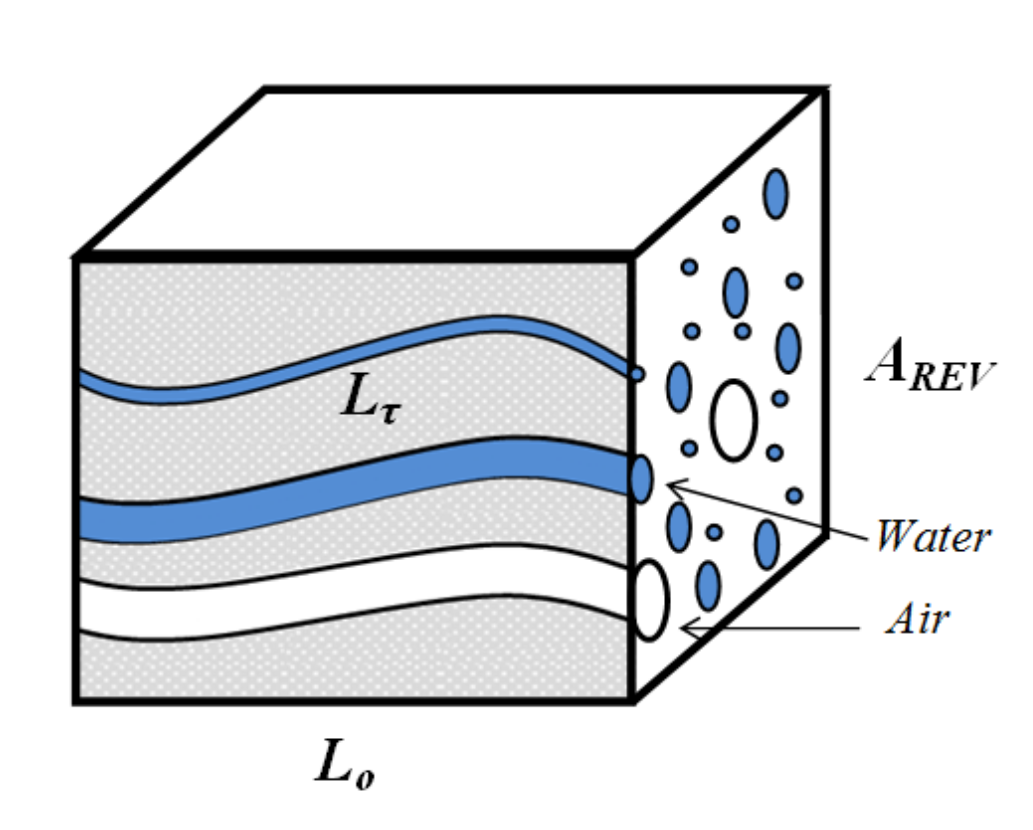
where $\Delta P$ (Pa) is the pressure difference across the capillary and $L_{\tau }$ (m) is the real length of the tortuous capillary (see Figure 1). Because the length of the porous media $L_o$ (m) is related to the real length of the tortuous capillary $L_{\tau }$ by the relation $L_{\tau }$= $\tau$$L_o$ in which $\tau$ (no units) is the tortuosity of the capillary (see, e.g., [85]). Note that the length of the capillaries in this work is assumed to be independent of the capillary radius and therefore $\tau$ is the same for all capillaries (see, e.g., [54]). Equation (6) is now rewritten as

$$i_s\left(r\right)=-\frac{\pi {ϵ}_r{ϵ}_o\zeta }{\eta }\frac{\Delta P}{L_o\tau }{r}^2.$$

(7)

The conduction current in the water occupied capillary tube under an electrical potential difference ($\Delta V$) is given by

$$i_c\left(r\right)=G_{tube}\Delta V,$$

(8)

where $G_{tube}$ (S) is the electrical conductance of the water occupied capillary. The electrical conductivity of a single capillary is given by the sum of the bulk and surface electrical conductivities. Note that the capillary may be occupied by either water or air. In capillaries occupied by water, surface conductivity occurs only at the interface between water and the solid, in which case ${\Sigma }_s$ (S) denotes the specific surface conductance of this interface. In capillaries occupied by air, surface conductivity again occurs at the interface between a thin wetting phase layer (i.e., an irreductible water film) and the solid. Consequently, in capillaries occupied by air, ${\Sigma }_{sa}$ (S) denotes the specific surface conductance due to solid-water interfaces [54,61]. Therefore, Equation (8) is given by

$$i_c\left(r\right)=\left\{\begin{array}{cc}\left[\frac{{\sigma }_w\pi r^2}{L_o\tau }+\frac{{\Sigma }_{s}2\pi r}{L_o\tau }\right]\Delta V\hfill & \mathrm{for}\mathrm{a}\mathrm{water}\mathrm{occupied}\mathrm{capillary}\hfill \\ \frac{{\Sigma }_{sa}2\pi r}{L_o\tau }\Delta V\hfill & \mathrm{for}\mathrm{an}\mathrm{air}\mathrm{occupied}\mathrm{capillary}\hfill \end{array}\right.$$

(9)

2.2. REV Scale

In order to develop the model for the SPCC under partially saturated conditions, we consider a representative elementary volume (REV) of a porous medium as a cube with a length $L_o$ (see Figure 1). As stated in literature (see, e.g., [86,87,88]), a porous medium exhibits fractal properties and can be conceptualized as a bundle of tortuous capillaries with different sizes from a minimum pore radius $r_{min}$ (m) to a maximum pore radius $r_{max}$ (m). It has been proved that the number of pores with radius from r to $r+dr$ in porous media is given by (see, e.g., [64,88])

$$-dN=D{r}_{max}^D{r}^{-D-1}dr,$$

(10)

where D (no units) is the fractal dimension for pore space. The negative sign implies that the number of pores decreases with the increase of pore size. Note that this is an equivalent pore size distribution that allows to reproduce the behavior of real porous media by simplifying the complexity of real pore networks. The pore fractal dimension D can be determined by a box-counting method (see, e.g., [88,89]). Additionally, D can also be estimated from the following the relation (see, e.g., [88,89]),

$$D=2-\frac{\ln \varphi }{\ln \alpha },$$

(11)

where $\varphi$ (no units) is the porosity of porous media and $\alpha$ = $r_{min}/r_{max}$ (no units).

We consider the REV under at varying saturation conditions. Then, contribution to the water flow depends on the effective saturation that is given by

$$\begin{array}{c}\hfill S_e=\frac{S_w-S_{wirr}}{1-S_{wirr}},\end{array}$$

(12)

where $S_w$ (no units) and $S_{wirr}$ (no units) are the water saturation and irreducible water saturation, respectively.

We assume that the REV is initially fully saturated and then drained when it experiences a pressure head h (m). For a capillary tube, the pore radius $r_h$ (m) is linked to the pressure head h by [90]

$$h=\frac{2T_s\cos \beta }{{\rho }_{w}g{r}_h},$$

(13)

where $T_s$ (N/m) is the fluid surface tension, $\beta$ (^o) is the contact angle, ${\rho }_w$ (kg/m${}^3$) is the fluid density, and g (m/s${}^2$) is the acceleration due to gravity. A capillary becomes fully desaturated if its radius r (m) is greater than the radius $r_h$ given by Equation (13). Therefore, it is reasonable to assume that capillaries with radii r between $r_{min}$ and $r_h$ will remain fully saturated.

For porous media containing only large and regular pores, the irreducible water saturation can often be neglected. For porous media containing small pores, the irreducible water saturation can be quite significant. This amount of water is taken into account in the model by setting irreducible water radius of capillaries $r_{wirr}$ (m). Consequently, the following assumptions are made in this work; (1) for $r_{min}\le r\le r_{wirr}$, the capillaries are occupied by water and are immobile (i.e., no film flow). Therefore, water does not contribute to the streaming current. However, water is electrically conductive, so it contributes to the conduction current. (2) For $r_{wirr}<r\le r_h$, the capillaries are occupied by water that is mobile, so they contribute to both the streaming current and the conduction current. (3) For $r_h<r\le r_{max}$, the capillaries are occupied by air, so does not contribute to the streaming current but contribute to the conduction current. In this work, film bound water, which adheres to the pore wall because of the molecular forces acting on the hydrophilic rock surface, in the capillaries with radius greater than $r_{wirr}$ is ignored in water saturation calculations. Therefore, the water saturation is defined as

$$\begin{array}{c}\hfill S_w=\frac{{\int }_{r_{min}}^{r_h}\pi r^2{L}_{\tau }(-dN)}{{\int }_{r_{min}}^{r_{max}}\pi r^2{L}_{\tau }(-dN)}=\frac{r_h^{2-D}-r_{min}^{2-D}}{r_{max}^{2-D}-r_{min}^{2-D}}.\end{array}$$

(14)

The irreducible water saturation is determined as

$$\begin{array}{c}\hfill S_{wirr}=\frac{{\int }_{r_{min}}^{r_{wirr}}\pi r^2{L}_{\tau }(-dN)}{{\int }_{r_{min}}^{r_{max}}\pi r^2{L}_{\tau }(-dN)}=\frac{r_{wirr}^{2-D}-r_{min}^{2-D}}{r_{max}^{2-D}-r_{min}^{2-D}}.\end{array}$$

(15)

From Equations (14) and (15), one has

$$r_h=r_{max}{\left[{\alpha }^{2-D}+S_w(1-{\alpha }^{2-D})\right]}^{\frac{1}{2-D}},$$

(16)

and

$$r_{wirr}=r_{max}{\left[{\alpha }^{2-D}+S_{wirr}(1-{\alpha }^{2-D})\right]}^{\frac{1}{2-D}}$$

(17)

where $\alpha$ = $r_{min}$/$r_{max}$.

The streaming current through the REV is the sum of the streaming currents over all water occupied capillaries with radius between $r_{wirr}$ and $r_h$ and given by

$$\begin{array}{cc}\hfill I_s=& {\int }_{r_{wirr}}^{r_h}{i}_s\left(r\right)(-dN)=\hfill \\ \hfill & -{\int }_{r_{wirr}}^{r_h}\frac{\pi {ϵ}_r{ϵ}_o\zeta }{\eta }\frac{\Delta P}{L_o\tau }D{r}_{max}^D{r}^{1-D}dr=\hfill \\ \hfill & -\frac{\pi {ϵ}_r{ϵ}_o\zeta }{\eta }\frac{\Delta P}{L_o\tau }\frac{D}{2-D}{r}_{max}^D(r_h^{2-D}-r_{wirr}^{2-D}).\hfill \end{array}$$

(18)

The conduction current through the REV is given by

$$\begin{array}{cc}\hfill I_c=& {\int }_{r_{min}}^{r_h}{i}_c\left(r\right)(-dN)\mathrm{d}r+{\int }_{r_h}^{r_{max}}{i}_c\left(r\right)(-dN)\mathrm{d}r=\hfill \\ \hfill & {\int }_{r_{min}}^{r_h}\Delta V\left[\frac{{\sigma }_w\pi r^2}{L_o\tau }+\frac{{\Sigma }_{s}2\pi r}{L_o\tau }\right](-dN)\mathrm{d}r+{\int }_{r_h}^{r_{max}}\Delta V\frac{{\Sigma }_{sa}2\pi r}{L_o\tau }(-dN)\mathrm{d}r.\hfill \end{array}$$

(19)

Evaluating integrals in Equation (19) yields

$$\begin{array}{cc}\hfill I_c=& \frac{\Delta VD\pi r_{max}^D}{L_o\tau }\left[\frac{{\sigma }_w(r_h^{2-D}-r_{min}^{2-D})}{2-D}+\frac{2{\Sigma }_s(r_h^{1-D}-r_{min}^{1-D})}{1-D}+\frac{2{\Sigma }_{sa}(r_{max}^{1-D}-r_h^{1-D})}{1-D}\right].\hfill \end{array}$$

(20)

Under steady-state conditions, the total streaming current $I_s$ (A) is equal to the total conduction current $I_c$ (A) through the REV in magnitude. Therefore, the following is obtained,

$$I_s=-I_c.$$

(21)

Combining Equations (18), (20), and (21) yields

$$\Delta V=\frac{{ϵ}_r{ϵ}_0\zeta \Delta P\frac{(r_h^{2-D}-r_{wirr}^{2-D})}{2-D}}{\eta \left[\frac{{\sigma }_w(r_h^{2-D}-r_{min}^{2-D})}{2-D}+\frac{2{\Sigma }_s(r_h^{1-D}-r_{min}^{1-D})}{1-D}+\frac{2{\Sigma }_{sa}(r_{max}^{1-D}-r_h^{1-D})}{1-D}\right]}$$

(22)

The SPCC at saturation is defined as

$$C_S=\frac{\Delta V}{\Delta P}=\frac{{ϵ}_r{ϵ}_0\zeta \frac{(r_h^{2-D}-r_{wirr}^{2-D})}{2-D}}{\eta \left[\frac{{\sigma }_w(r_h^{2-D}-r_{min}^{2-D})}{2-D}+\frac{2{\Sigma }_s(r_h^{1-D}-r_{min}^{1-D})}{1-D}+\frac{2{\Sigma }_{sa}(r_{max}^{1-D}-r_h^{1-D})}{1-D}\right]}$$

(23)

Substituting Equations (16) and (17) into Equation (23) and doing some arrangements, the following is obtained,

$$\begin{array}{cc}\hfill C_S\left(S_w\right)=& \frac{{ϵ}_r{ϵ}_0\zeta (S_w-S_{wirr})}{\eta \left[{\sigma }_w{S}_w+\frac{2{\Sigma }_s}{r_{max}}\frac{2-D}{1-D}\frac{\left[{(S_w(1-{\alpha }^{2-D})+{\alpha }^{2-D})}^{\frac{1-D}{2-D}}-{\alpha }^{1-D}\right]}{1-{\alpha }^{2-D}}+\frac{2{\Sigma }_{sa}}{r_{max}}\frac{2-D}{1-D}\frac{\left[1-{(S_w(1-{\alpha }^{2-D})+{\alpha }^{2-D})}^{\frac{1-D}{2-D}}\right]}{1-{\alpha }^{2-D}}\right]}.\hfill \end{array}$$

(24)

The wetting layer of water contributes to the surface electrical conductivity even in capillaries occupied by air. Following the work in [54], we assume that the presence of air does not modify surface conductivity at the solid water interface and ${\Sigma }_{sa}={\Sigma }_s$. Consequently, Equation (24) becomes

$$C_S\left(S_w\right)=\frac{{ϵ}_r{ϵ}_0\zeta (S_w-S_{wirr})}{\eta \left[{\sigma }_w{S}_w+\frac{2{\Sigma }_s}{r_{max}}\frac{2-D}{1-D}\frac{1-{\alpha }^{1-D}}{1-{\alpha }^{2-D}}\right]}.$$

(25)

Equation (25) indicates that the SPCC under partially saturated conditions is related to the zeta potential, the fluid relative permittivity, viscosity, water saturation, irreducible water saturation, fluid electrical conductivity, and the surface conductance at the solid water interface. Additionally, Equation (25) is related to the microstructural parameters of a porous medium (D, $\alpha$, $r_{max}$).

In case of full saturation and zero irreducible water saturation ($S_w$ = 1 and $S_{wirr}$ = 0), Equation (25) reduces to

$$C_S(S_w=1)=\frac{{ϵ}_r{ϵ}_0\zeta }{\eta \left[{\sigma }_w+\frac{2{\Sigma }_s}{r_{max}}\frac{2-D}{1-D}\frac{1-{\alpha }^{1-D}}{1-{\alpha }^{2-D}}\right]}.$$

(26)

Equation (26) has been well validated by the authors of [64] for consolidated porous samples. Note that Equation (26) has the similar form as proposed by Morgan et al. [68] or Waxman and Smits [91]:

$$C_S(S_w=1)=\frac{{ϵ}_r{ϵ}_0\zeta }{\eta \left[{\sigma }_w+F{\sigma }_s\right]},$$

(27)

where F is the formation factor and ${\sigma }_s$ is the surface conductivity.

In the case of zero irreducible water saturation and negligible surface conductivity ($S_{wirr}$ = 0 and ${\Sigma }_s$ = 0), Equation (25) reduces to the HS equation (see Equation (2))

$$C_S\left(S_w\right)=\frac{{ϵ}_r{ϵ}_0\zeta }{\eta {\sigma }_w}.$$

(28)

Equation (28) indicates that the SPCC does not depend on water saturation in this very specific case (i.e., $S_{wirr}$ = 0 and ${\Sigma }_s$ = 0). This prediction is the same as that stated by [54] (see his Figure 3a).

2.3. Relative Streaming Potential Coupling Coefficient

From Equation (25), the relative SPCC is obtained as

$$C_{rel}=\frac{C_S\left(S_w\right)}{C_S(S_w=1)}=\frac{\frac{S_w-S_{wirr}}{1-S_{wirr}}}{\frac{\left[{\sigma }_w{S}_w+\frac{2{\Sigma }_s}{r_{max}}\frac{2-D}{1-D}\frac{1-{\alpha }^{1-D}}{1-{\alpha }^{2-D}}\right]}{\left[{\sigma }_w+\frac{2{\Sigma }_s}{r_{max}}\frac{2-D}{1-D}\frac{1-{\alpha }^{1-D}}{1-{\alpha }^{2-D}}\right]}}.$$

(29)

For negligible surface conductivity, Equation (29) becomes

$$C_{rel}=\frac{(S_w-S_{wirr})}{(1-S_{wirr})S_w}=\frac{S_e}{S_w}.$$

(30)

Equations (29) and (30) indicate the dependence of $C_{rel}$ (no units) on water saturation $S_w$ (no units). In addition, Equation (30) shows that when the surface conductivity is negligible, $C_{rel}$ only depends on $S_w$ and $S_{wirr}$ (no units) regardless of ${\sigma }_w$ (S/m), D (no units), $r_{max}$ (no units), and $\alpha$ (no units).

2.4. The Relation Between SPCC and Effective Excess Charge Density

The effective excess charge density ${\widehat{Q}}_v^{REV}$ (C/m${}^3$) carried by the water flow in the REV is calculated based on the same approach proposed by [59,92]

$${\widehat{Q}}_v^{REV}=\frac{1}{v_D{A}_{REV}}{\int }_{r_{wirr}}^{r_h}{\widehat{Q}}_v^r\overline{v}\left(r\right)\pi r^2(-dN),$$

(31)

where $v_D$ (m/s) is the Darcy velocity, $A_{REV}$ (m${}^2$) is the cross-sectional area of the REV, ${\widehat{Q}}_v^r$ (C/m${}^3$) is the effective excess charge density carried by the water flow in a single water occupied capillary of radius r (m), and $\overline{v}$ (m/s) is the average velocity in the capillary. As shown by [59], $v_D$ is given as

$$v_D=\frac{\Delta Pk{k}_{rel}}{\eta L_o},$$

(32)

where k (m${}^2$) and $k_{rel}$ (no units) are the permeability and relative permeability of the REV, respectively. Under the thin EDL assumption, ${\widehat{Q}}_v^r$ is given by [92]

$${\widehat{Q}}_v^r=-\frac{8{ϵ}_r{ϵ}_0\zeta }{r^2}.$$

(33)

Additionally, $\overline{v}$ is given by (see, e.g., [59])

$$\overline{v}\left(r\right)=\frac{\Delta P{r}^2}{8\eta \tau L_o}.$$

(34)

Substituting Equations (32)–(34) into Equation (31) and doing some arrangements, one obtains

$${\widehat{Q}}_v^{REV}=-\frac{{ϵ}_r{ϵ}_0\zeta }{\tau k{k}_{rel}}\frac{\pi D}{(2-D)A_{REV}}{r}_{max}^D{r}_{max}^{2-D}(S_w-S_{wirr})(1-{\alpha }^{2-D}).$$

(35)

In addition, the electrical conductivity of the REV at saturation is calculated as

$$\sigma =\frac{L_o}{A_{REV}{R}_{REV}},$$

(36)

where $R_{REV}$ ($\Omega$) is the resistance of the REV that can be deduced from Equation (20) using Ohm${}^{\prime }$s law:

$$\frac{1}{R_{REV}}=\frac{I_c}{\Delta V}=\frac{D\pi r_{max}^D}{L_o\tau }\left[\frac{{\sigma }_w(r_h^{2-D}-r_{min}^{2-D})}{2-D}+\frac{2{\Sigma }_s(r_h^{1-D}-r_{min}^{1-D})}{1-D}+\frac{2{\Sigma }_{sa}(r_{max}^{1-D}-r_h^{1-D})}{1-D}\right].$$

(37)

Using ${\Sigma }_s={\Sigma }_{sa}$ and applying the same above mentioned approach, Equation (37) is rewritten as

$$\frac{1}{R_{REV}}=\frac{D\pi r_{max}^D{r}_{max}^{2-D}(1-{\alpha }^{2-D})}{L_o\tau (2-D)}\left[{\sigma }_w{S}_w+\frac{2{\Sigma }_s}{r_{max}}\frac{2-D}{1-D}\frac{1-{\alpha }^{1-D}}{1-{\alpha }^{2-D}}\right].$$

(38)

Combining Equations (36) and (38), the following is obtained,

$$\sigma \left(S_w\right)=\frac{\pi D{r}_{max}^2(1-{\alpha }^{2-D})}{A_{REV}\tau (2-D)}\left[{\sigma }_w{S}_w+\frac{2{\Sigma }_s}{r_{max}}\frac{2-D}{1-D}\frac{1-{\alpha }^{1-D}}{1-{\alpha }^{2-D}}\right].$$

(39)

From Equations (25), (35), and (39), one has

$$C_S\left(S_w\right)=-\frac{{\widehat{Q}}_v^{REV}\left(S_w\right)k{k}_{rel}\left(S_w\right)}{\eta \sigma \left(S_w\right)}.$$

(40)

Equation (40) is the same as that reported in literature using different approaches such as the volume-averaging upscaling (see, e.g., [51,55,83]). However, in this work, we obtain that based on the fractal theory for porous media and the capillary tube model.

From Equation (39), the relative electrical conductivity is obtained as

$${\sigma }_{rel}\left(S_w\right)=\frac{\sigma \left(S_w\right)}{\sigma (S_w=1)}=\frac{{\sigma }_w{S}_w+\frac{2{\Sigma }_s}{r_{max}}\frac{2-D}{1-D}\frac{1-{\alpha }^{1-D}}{1-{\alpha }^{2-D}}}{{\sigma }_w+\frac{2{\Sigma }_s}{r_{max}}\frac{2-D}{1-D}\frac{1-{\alpha }^{1-D}}{1-{\alpha }^{2-D}}}.$$

(41)

Comparing Equations (29) and (41) yields the following

$$C_{rel}=\frac{S_e}{{\sigma }_{rel}\left(S_w\right)}.$$

(42)

Equation (42) is exactly the same as that proposed by the authors of [54,59].

2.5. Johnson Length

Comparing Equations (3) and (26), a new expression for the characteristic length scale (Johnson length) $\mathrm{\Lambda }$ (m) under fully saturated conditions is obtained as

$$\mathrm{\Lambda }=r_{max}\frac{(1-D)(1-{\alpha }^{2-D})}{(2-D)(1-{\alpha }^{1-D})}=r_{max}\frac{(1-D)(1-\varphi )}{(2-D)(1-{\alpha }^{1-D})}.$$

(43)

It should be noted that ${\alpha }^{2-D}=\varphi$.

There have been published models relating the $\mathrm{\Lambda }$ (m) to the grain diameter d (m). One is presented by [93,94]

$$\mathrm{\Lambda }=\frac{d}{2m(F-1)}\approx \frac{d}{2mF},$$

(44)

where F (no units) is the formation factor, m (no units) is the cementation exponent of porous media. For spherical grain based samples, m is stated to be 1.5 (see, e.g., [95]).

Equation (43) is related to microstructural properties of porous materials (D, $\varphi$, $\alpha$, $r_{max}$). Therefore, it indicates more mechanisms affecting the $\mathrm{\Lambda }$ (m) than Equation (44). There is no empirical constants in Equation (43), but there are two in Equation (44) (F and m).

The effective pore radius is linked to the characteristic length scale by [96]

$$r_{eff}=\mathrm{\Lambda }\sqrt{\frac{8}{a}},$$

(45)

where a (no units) is a constant and normally taken as to 8/3 for spherical grain based samples [94,96].

Combining Equations (43) and (45), the $r_{eff}$ (m) can be expressed in terms of microstructural parameters of porous materials as follows:

$$r_{eff}=r_{max}\frac{(1-D)(1-\varphi )}{(2-D)(1-{\alpha }^{1-D})}\sqrt{\frac{8}{a}}.$$

(46)

Combining Equations (44) and (45), the $r_{eff}$ (m) is expressed in terms of F and m as follows,

$$r_{eff}=\frac{d}{2m(F-1)}\sqrt{\frac{8}{a}}\approx \frac{d}{2mF}\sqrt{\frac{8}{a}}.$$

(47)

3. Results and Discussion

3.1. Relative Streaming Potential Coupling Coefficient

Figure 2 shows the variation of the relative SPCC with water saturation predicted from Equation (30) for three values of irreducible water saturation $S_{wirr}$. It is seen that $C_{rel}$ increases with increasing water saturation $S_w$ as observed in literature (see, e.g., [48,50,58]). When $S_{wirr}$ = 0, $C_{rel}$ is always equal 1, meaning that the SPCC does not depend on water saturation as predicted by [54]. In addition, $C_{rel}$ is very sensitive with $S_{wirr}$ ($C_{rel}$ decreases with an increase of $S_{irr}$ at the same water saturation). The reason is that at the same water saturation there are less capillaries occupied by water that is mobile for the electrokinetic effect when $S_{irr}$ increases.

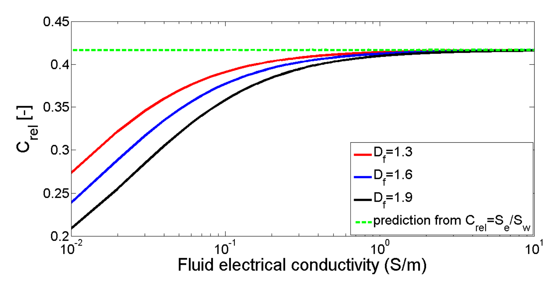
Figure 3 shows the variation of the relative SPCC ($C_{rel}$) with fluid electrical conductivity (${\sigma }_w$) based on Equation (29) for three different values of D (1.3, 1.6, and 1.9). Input parameters for modeling are ${\Sigma }_s$ = 10 × 10${}^{-9}$ S that is a typical value reported in literature (see, e.g., [97,98,99]), $S_{wirr}$ = 0.2, $S_w$ = 0.3, $r_{max}$ = 50.10${}^{-6}$ m and $\alpha$ = 0.01. It is seen that the relative SPCC increases with increasing electrical conductivity at low electrical conductivity for all three values of D. However, at high fluid electrolyte conductivity (${\sigma }_w\approx$ 1 S/m), the relative SPCC becomes independent of D that is linked to grain texture of porous media. The reason is that at high fluid electrical conductivity the surface conductivity is negligible, the $C_{rel}$ is now determined by Equation (30) and is independent of ${\sigma }_w$ and D (see the dashed line in Figure 3). Additionally, it is seen that $C_{rel}$ decreases with an increase of D at low fluid electrical conductivity.

If pore size distribution is not known, one can estimate the maximum pore radius with the knowledge of the mean grain diameter d of porous materials as [100]

$$r_{max}=\frac{d}{8}\left[\sqrt{\frac{2\varphi }{1-\varphi }}+\sqrt{\frac{\varphi }{1-\varphi }}+\sqrt{\frac{\pi }{4(1-\varphi })}-1\right],$$

(48)

Equation (48) has been justified by a good agreement with experimental data as shown in the recent work (see, e.g., [64,65]). Equation (48) will be used to determine $r_{max}$ in later modelings.

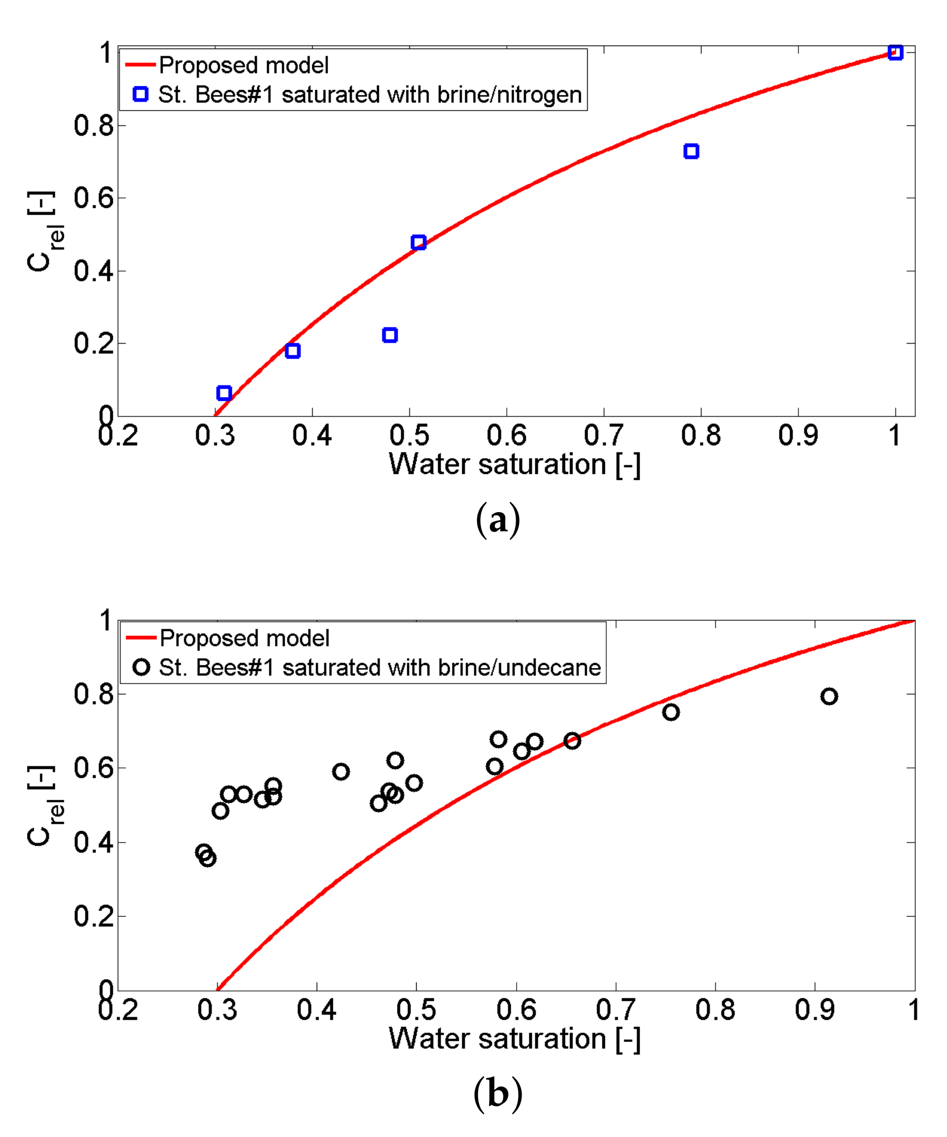
Vinogradov and Jackson [58] measured $C_{rel}$ as a function of $S_w$ for the St. Bees sample saturated with brine/nitrogen and brine/undecane (see symbols in Figure 4). When the sample is saturated with brine/nitrogen, $C_{rel}$ is observed to approach zero at the irreducible water saturation ($S_{wirr}$ = 0.3) as indicated in Figure 4a. The brine used in [58] was a simple 0.01 M solution of NaCl. Therefore, to estimate the fluid elecrical conductivity, we use the relation ${\sigma }_w=10\times C_f$ = 0.1 S/m for a NaCl solution in the range of electrolyte concentration $C_f$ between 10${}^{-6}$ M and 1 M temperature between 15 ${}^{\circ }$C and 25 ${}^{\circ }$C [101]. With fluid electrical conductivity of 0.1 S/m, the surface conductivity is not safely neglected for the same system of the sample and fluid as reported in [33] in which the surface conductivity is negligible for ${\sigma }_w$ larger than 1 S/m. Therefore, we use Equation (29) to reproduce the experimental data in Figure 4a (see the solid line) with $S_{wirr}$ = 0.3, d = 130 $\mathsf{\mu }$m, $\varphi$ = 0.19, ${\sigma }_w$ = 0.1 S/m which are obtained from [58], ${\Sigma }_s$ = 10×10${}^{-9}$ S (typical value for silica based rocks in contact with NaCl solutions) and $\alpha$ = 0.01 (best fit). A good agreement between the model and experimental data is observed. Note that D is determined from Equation (11) with the knowledge of $\varphi$ and $\alpha$; $r_{max}$ is determined from Equation (48) with the knowledge of $\varphi$ and d.

However, Vinogradov and Jackson [58] observed that the relative SPCC gets the non-zero value at the irreducible water saturation as shown in Figure 4b for brine/undecane. That observation may be due to the movement of brine along with the undecane within the wetting layers of the pores [102]. That effect is important at low brine saturation (wetting phase). The small volumes of flowing brine are hard to be measured and therefore the brine saturation seems to be unchanging. However, the brine contains a very high density of excess electrical charge [44,58]. Consequently, the streaming current is considerable, leading to a non-zero streaming potential at the irreducible water saturation. One can note that the proposed model is valid for porous media saturated by water (brine)/air (nitrogen). The reason is that the model is developed based on assumption of water-wet capillaries saturated with water and a nonwetting phase such as air as mentioned in Section 2.

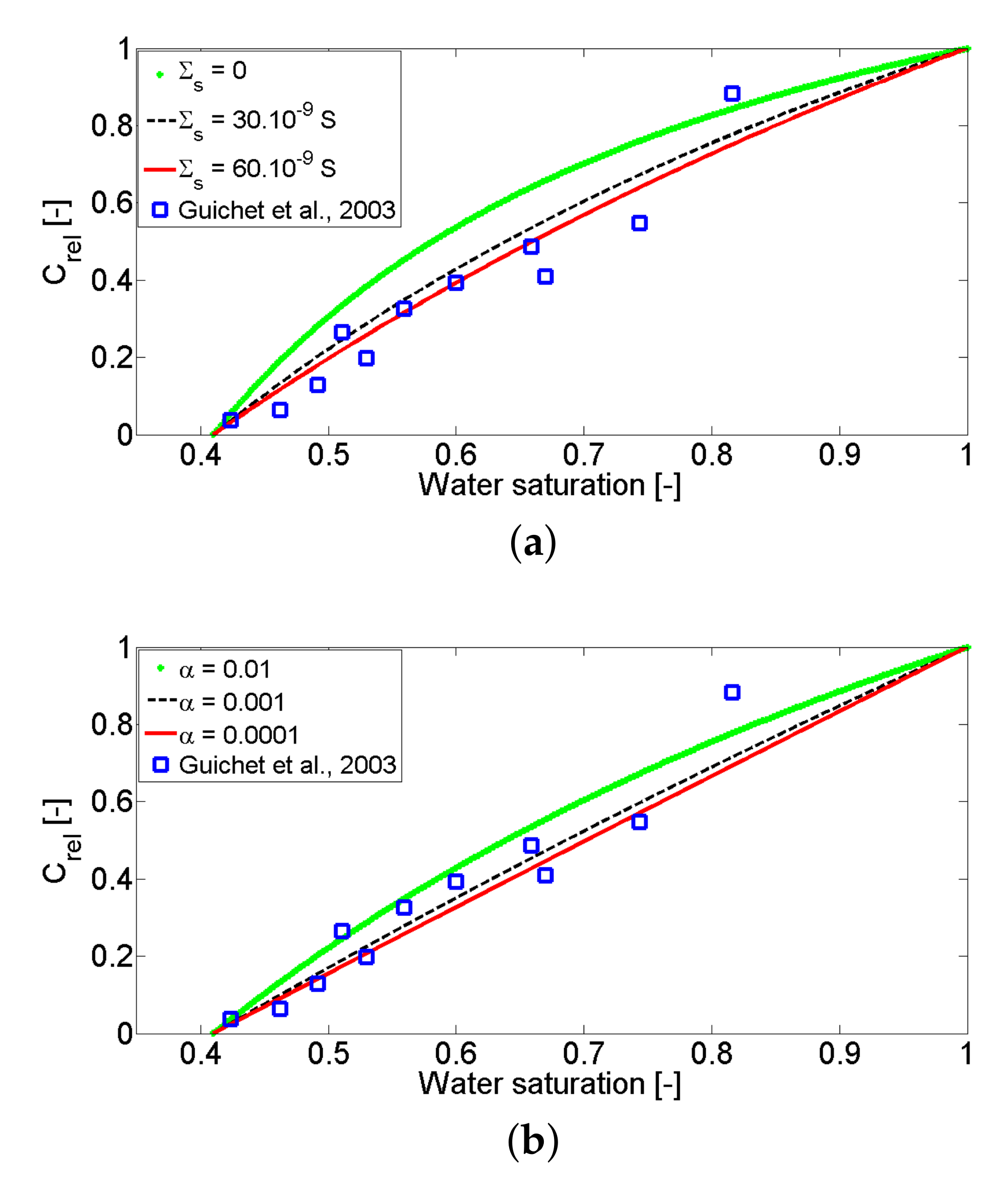
Figure 5 shows experimental data of $C_{rel}$ as a function of $S_w$ for a sand column saturated with brine/argon (see symbols) obtained from [48]. The experimental data is explained by the model given by Equation (29) (see the lines). To see how sensitive the model is with ${\Sigma }_s$ and $\alpha$, three different values of ${\Sigma }_s$ (0, 30 × 10${}^{-9}$ S and 60 × 10${}^{-9}$ S) and three different values of $\alpha$ (0.01, 0.001, and 0.0001) are applied for modeling (see Figure 5a,b, respectively). Input parameters for modeling are $S_{wirr}$ = 0.41, d = 300 $\mathsf{\mu }$m, $\varphi$ = 0.4, ${\sigma }_w$ = 0.01 S/m that are taken from [48]. In Figure 5a, $\alpha$ = 0.01 is used and in Figure 5b, ${\Sigma }_s$ = 30 × 10${}^{-9}$ S is used. It is seen that the model is very sensitive with ${\Sigma }_s$ and $\alpha$. A good agreement between the experimental data and the model is obtained with $\alpha$ = 0.01 and ${\Sigma }_s$ = 30 × 10${}^{-9}$ S. Note that $\alpha$ = 0.01 are normally relevant for unconsolidated samples of sand grains (see, e.g., [64,65,88]) and ${\Sigma }_s$ = 30 × 10${}^{-9}$ S is of the same order of magnitude as those reported in published work (see, e.g., [76,97,103]).

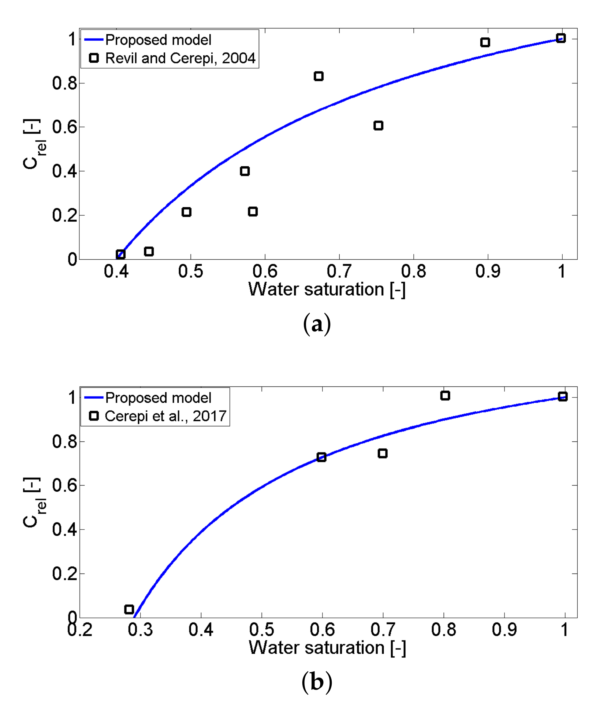
Figure 6 shows experimental data of $C_{rel}$ as a function of $S_w$ for the samples E39 and E3 saturated with brine/nitrogen obtained from the work in [50] and the sample of Brauvilliers limestone saturated with brine/nitrogen obtained from the work in [83] (see symbols in Figure 6a,b, respectively). Equation (30) is applied to explain the experimental data because the fluid electrical conductivities in both cases are reported to be large enough to ignore the surface conductivity (${\sigma }_w$ = 0.93 S/m and 1.33 S/m). The solid lines are obtained from Equation (30) in which $S_{wirr}$ = 0.4 and $S_{wirr}$ = 0.29 are reported by the authors of [50,83], respectively. It is seen that the model predictions are in good agreement with the published data.

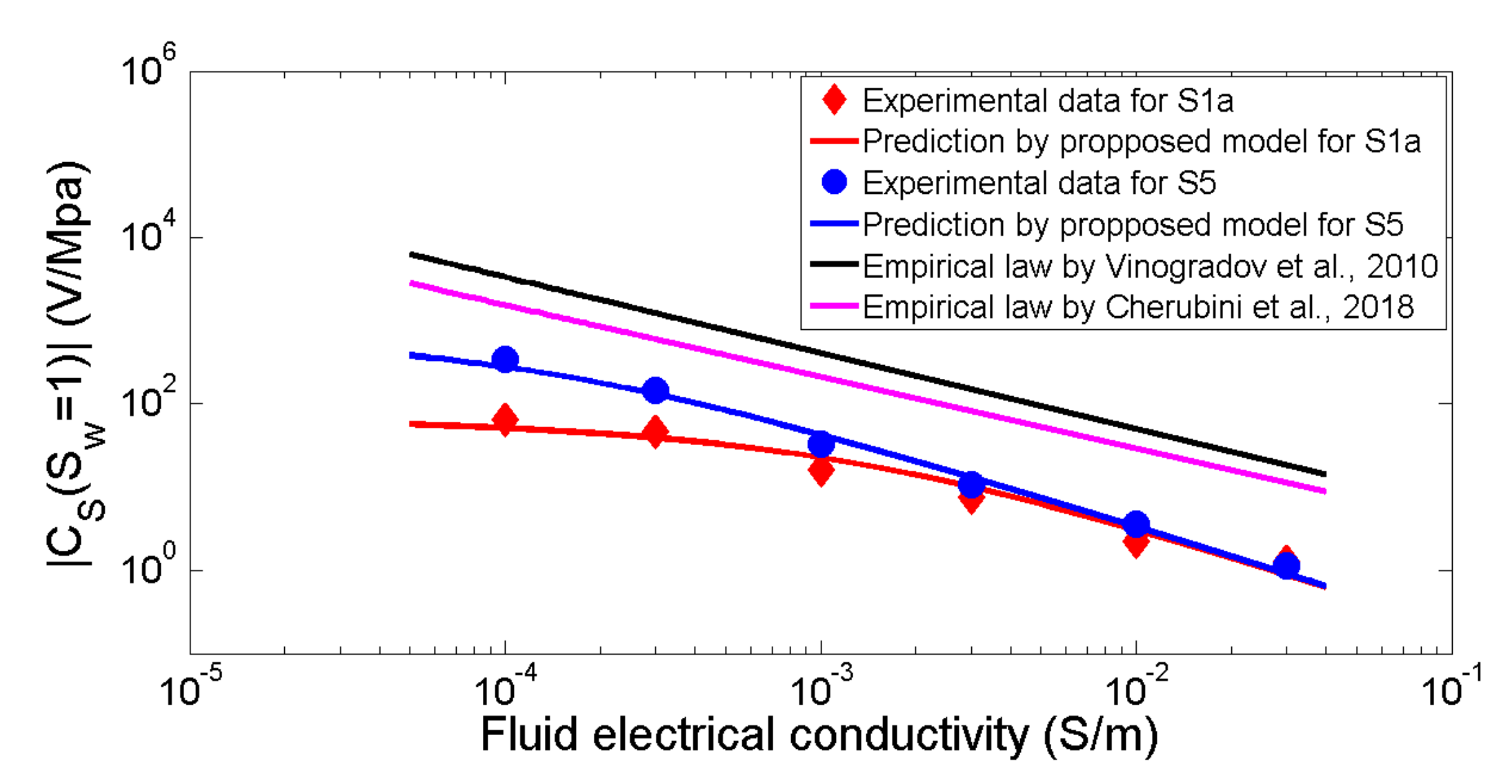
Figure 7 shows the dependence of the SPCC on the fluid electrical conductivity for two glass bead packs (S1a with d = 56 $\mathsf{\mu }$m and S5 with d = 512 $\mathsf{\mu }$m) saturated with NaCl solutions (see symbols) taken from [99] at full saturation. Equation (26) is used to explain the observed behavior, in which $\varphi$ is taken as 0.4 [99], ${\Sigma }_s$ = 10${}^{-9}$ S and $\alpha$ = 0.01 are used for the best fit. D and $r_{max}$ are determined in the same way as previously mentioned with the knowledge of $\varphi$, $\alpha$ and d. The dependence of the zeta potential on fluid electrical conductivity is based on the empirical expression $\zeta =-9.67+19.02{log}_{10}\left({\sigma }_w\right)$ (mV) given by [33]. It is seen that the model can reproduce the main trend of the published data. Additionally, two empirical laws between the SPCC (mV/MPa) and electrolyte concentration $C_f$ (mol/L) proposed by Vinogradov et al. [33] for sandstone ($C_S(S_w=1)=-1.36C_f^{-0.9123}$) and by Cherubini et al. [104] for Carbonate rocks ($C_S(S_w=1)=-1.41C_f^{-0.862}$) are used to reproduce the experimental data reported by [99] (see Figure 7). Recall that the relation ${\sigma }_w=10C_f$ is also used to deduce $C_f$ from ${\sigma }_w$. As seen in Figure 7, the empirical laws overestimate experimental data even they can explain the decrease of the SPCC with an increase of ${\sigma }_w$. The reason is that those laws were obtained by fitting experimental data with big data scattering (e.g., see Figure 10 of [33]). Therefore, the empirical laws may not work well for two single silica-based samples in a large range of electrical conductivity reported by [99]. In addition, the difference in expressions proposed by the authors of [33,104] indicates that the empirical law is largely mineral-dependent.

3.2. Johnson Length

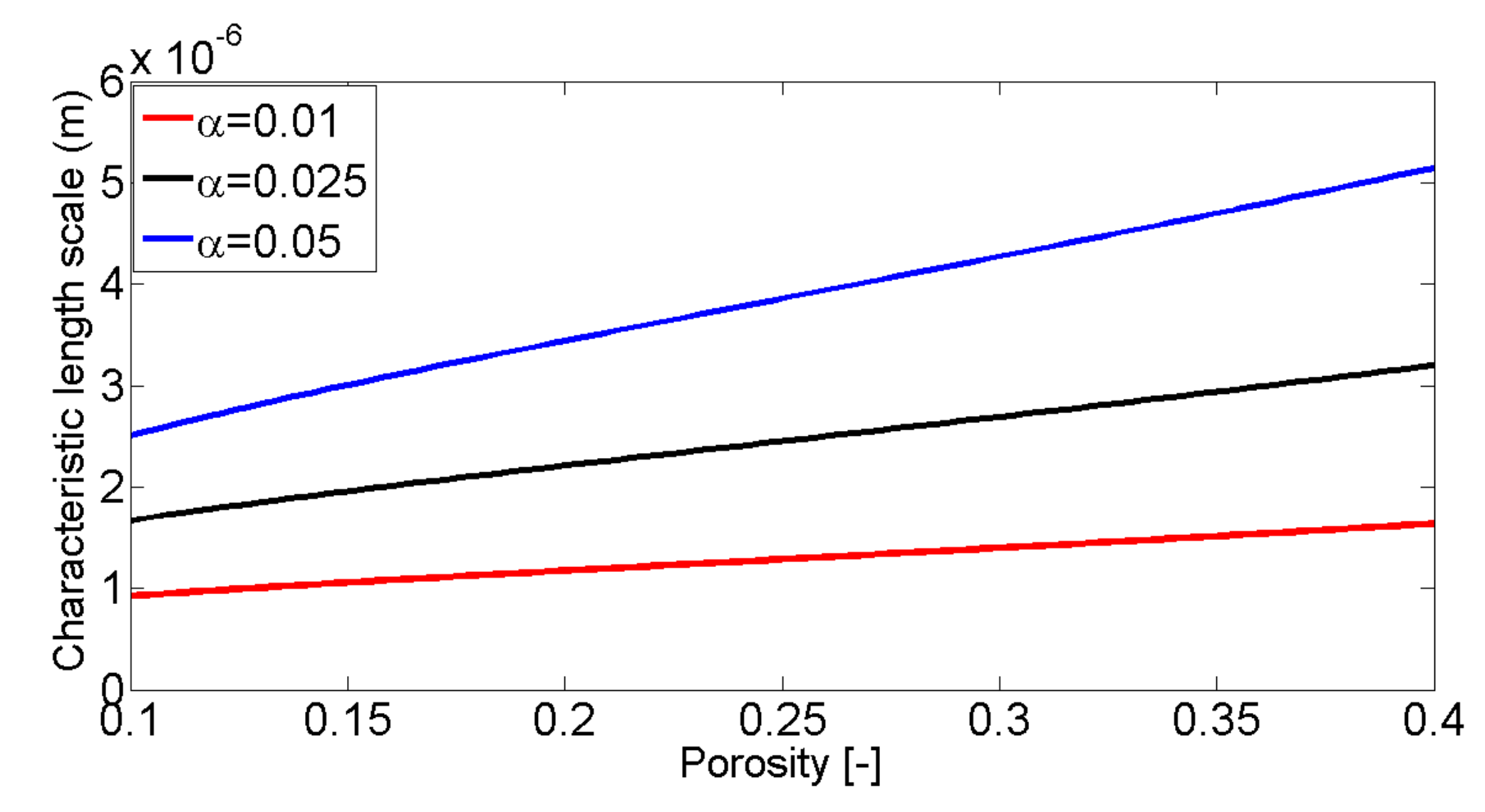
Figure 8 shows the variation of the characteristic length scale with porosity predicted from Equation (46) at three different values of $\alpha$ (0.01, 0.025, and 0.05) for d = 50 × 10${}^{-6}$ m. It is shown that the characteristic length scale is sensitive to the porosity $\varphi$ and the ratio $\alpha$ between $r_{min}$ and $r_{max}$.

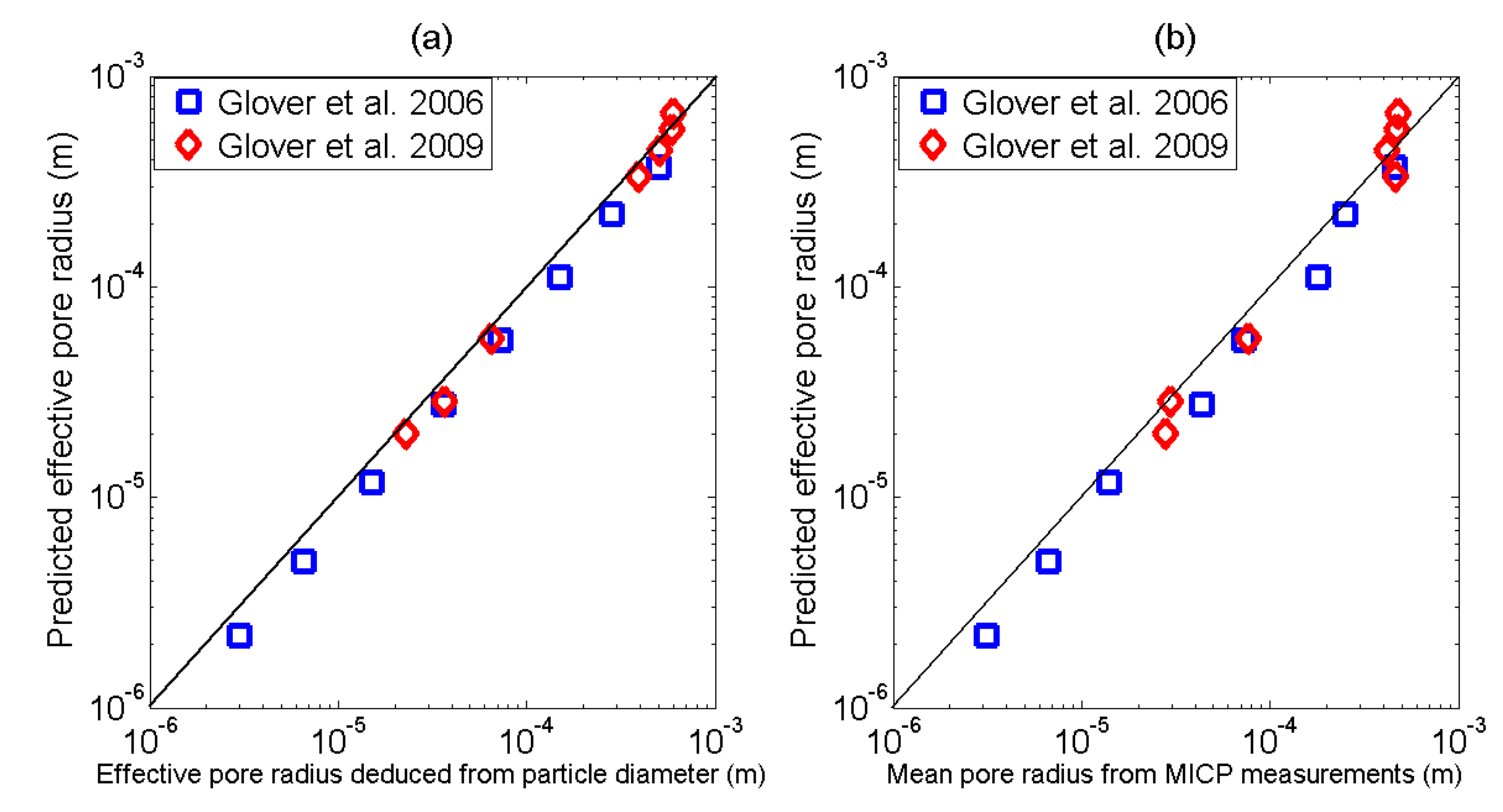
In Figure 9, we show (a) the comparison between effective pore radii predicted from the proposed model given by Equation (46) and those predicted from Equation (47) presented by [94,96] for a set of glass bead packs (see

Table 2. Properties for a set of glass bead packs reported in [94,96]. Symbols of d ($\mathsf{\mu }$m), $\varphi$ (no units), m (no units), and $r_{mean}$ ($\mathsf{\mu }$m) stand for the grain diameter, porosity, cementation exponent, and mean pore radius of glass bead samples from mercury injection capillary pressure (MICP) measurements, respectively.

Sample	d	$\mathit{\varphi }$	m	${\mathit{r}}_{\mathbf{mean}}$	Source
	($\mathsf{\mu }$m)	(no units)	(no units)	from MICP ($\mathsf{\mu }$m)
A	20	0.4009	1.49	3.12	[94]
B	45	0.3909	1.48	6.65	[94]
C	106	0.3937	1.50	14.04	[94]
D	250	0.3982	1.50	43.7	[94]
E	500	0.3812	1.46	72.3	[94]
F	1000	0.3954	1.47	180.2	[94]
G	2000	0.3856	1.49	252.6	[94]
H	3350	0.3965	1.48	459.3	[94]
I	3000	0.3978	1.56	463.1	[96]
J	4000	0.3854	1.55	419.7	[96]
K	5000	0.3756	1.57	476.2	[96]
L	6000	0.3566	1.62	480.0	[96]
M	256	0.3987	1.51	29.6	[96]
N	512	0.3890	1.56	76.9	[96]
O	181	0.3824	1.54	28.1	[96]

), and (b) the comparison between effective pore radii predicted from the proposed model given by Equation (46) and those from measurements of the mercury injection capillary pressure (MICP) for the same set of samples (see Table 2). It is seen that the proposed model given by Equation (46) is very good agreement with that presented by [94,96] or experimental data from the MICP measurements. It should be noted that in Equation (46), $\alpha$ is taken as 0.025 due to the best fit, D and $r_{max}$ are determined from (11) and Equation (48) as previously mentioned with the knowledge of $\alpha$, $\varphi$ and d (see Table 2). For modeling of Equation (46) and Equation (47), d and m are obtained from [94,96] and re-shown in Table 2, F is determined by the relation $F={\varphi }^{-m}$[105], and a is taken as 8/3.

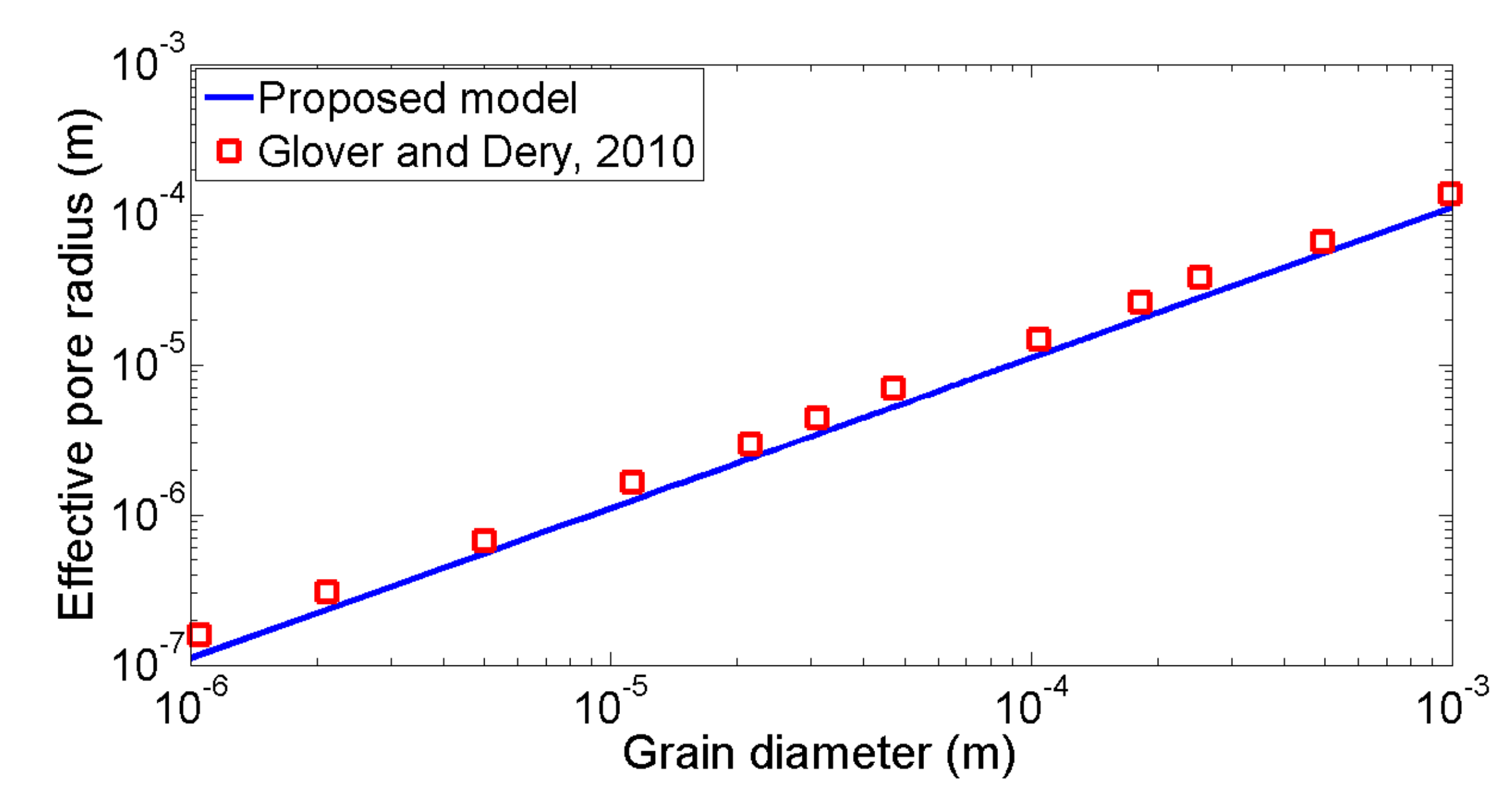
Similarly, Glover and Dery (2010) [76] applied Equation (47) for a set of glass bead packs to obtain the effective pore radii of the samples (see his Table 1). The properties and the effective pore radii obtained by [76] for all samples are re-shown in

Table 3. Properties for a set of glass bead packs reported in [76]. Symbols of d ($\mathsf{\mu }$m), $\varphi$ (no units), m (no units), F (no units), and $r_{eff}$ ($\mathsf{\mu }$m) stand for the grain diameter, porosity, cementation exponent, formation factor, and effective pore radius of the glass bead samples, respectively.

Sample	d	$\mathit{\varphi }$	m	F	${\mathit{r}}_{\mathbf{eff}}$	Source
	($\mathsf{\mu }$m)	(no units)	(no units)	(no units)	($\mathsf{\mu }$m)
1	1.05	0.411	1.5	3.80	0.16	[76]
2	2.11	0.398	1.5	3.98	0.31	[76]
3	5.01	0.380	1.5	4.27	0.68	[76]
4	11.2	0.401	1.5	3.94	1.64	[76]
5	21.5	0.383	1.5	4.23	2.94	[76]
6	31.0	0.392	1.5	4.07	4.40	[76]
7	47.5	0.403	1.5	3.91	7.02	[76]
8	104	0.394	1.5	4.04	14.86	[76]
9	181	0.396	1.5	4.01	26.04	[76]
10	252	0.414	1.5	3.75	38.53	[76]
11	494	0.379	1.5	4.28	66.64	[76]
12	990	0.385	1.5	4.18	136.62	[76]

. From that, the variation of effective pore radii with grain diameter is shown in Figure 10 (see symbols). The observation can be reproduced by Equation (46) (see solid line), in which $\alpha$ is taken as 0.025, D and $r_{max}$ are obtained in the same manner as previously mentioned with the knowledge of $\alpha$, $\varphi$, and d (see Table 3). It is seen that the model provides a fairy good agreement with experimental data.

4. Conclusions

We develop a physically based model for the SPCC as well as the relative SPCC during the flow of water and air in porous materials under partially saturated conditions by considering a bundle of tortuous capillaries with a fractal pore size distribution. From the obtained expressions, we obtain the familiar relation between the SPCC and the effective excess charge density that has been reported in literature using another approach. The proposed model for the SPCC and relative SPCC is related to fluid electrical conductivity, water saturation, irreducible water saturation, and microstructural parameters of porous media. In particular, the surface conductivity of porous media has been taken into account in the model. In addition, we also obtain an new expression for the characteristic length scale $\mathrm{\Lambda }$ at full saturation. The proposed model is then successfully validated using experimental data in literature. We believe that the models proposed in this work can be useful to study hydrogeological processes in the unsaturated zone such as infiltration, evaporation, or contaminant fluxes.

References

- Rubin, Y.; Hubbard, S. Hydrogeophysics; Springer: Berlin/Heidelberg, Germany, 2006. [Google Scholar]
- Hubbard, S.; Linde, N. Hydrogeophysics. In Treatise on Water Science; Wilderer, P., Ed.; Academic Press: Oxford, UK, 2011. [Google Scholar]
- Binley, A.; Hubbard, S.S.; Huisman, J.A.; Revil, A.; Robinson, D.A.; Singha, K.; Slater, L.D. The emergence of hydrogeophysics for improved understanding of subsurface processes over multiple scales. Water Resour. Res. 2015, 51, 3837–3866. [Google Scholar] [CrossRef] [PubMed] [Green Version]
- Revil, A.; Jardani, A. The Self-Potential Method: Theory and Applications in Environmental Geosciences; Cambridge University Press: Cambridge, UK, 2013. [Google Scholar]
- Jouniaux, L.; Pozzi, J.; Berthier, J.; Masse, P. Detection of fluid flow variations at the Nankai Trough by electric and magnetic measurements in boreholes or at the seafloor. J. Geophys. Res. 1999, 104, 29293–29309. [Google Scholar] [CrossRef]
- Fagerlund, F.; Heinson, G. Detecting subsurface groundwater flow infractured rock using self-potential (SP) methods. Environ. Geol. 2003, 43, 782–794. [Google Scholar] [CrossRef]
- Titov, K.; Revil, A.; Konosavsky, P.; Straface, S.; Troisi, S. Numerical modelling of self-potential signals associated with a pumping test experiment. Geophys. J. Int. 2005, 162, 641–650. [Google Scholar] [CrossRef]
- Aizawa, K.; Ogawa, Y.; Ishido, T. Groundwater flow and hydrothermal systems within volcanic edifices: Delineation by electric self-potential and magnetotellurics. J. Geophys. Res. 2009, 114. [Google Scholar] [CrossRef]
- Aubert, M.; Atangana, Q.Y. Self-Potential Method in Hydrogeological Exploration of Volcanic Areas. Groundwater 1996, 34, 1010–1016. [Google Scholar] [CrossRef]
- Finizola, A.; Lenat, N.; Macedo, O.; Ramos, D.; Thouret, J.; Sortino, F. Fluid circulation and structural discontinuities inside misti volcano (peru) inferred from sel-potential measurements. J. Volcanol. Geotherm. Res. 2004, 135, 343–360. [Google Scholar] [CrossRef] [Green Version]
- Mauri, G.; Williams-Jones, G.; Saracco, G. Depth determinations of shallow hydrothermal systems by self-potential and multi-scale wavelet tomography. J. Volcanol. Geotherm. Res. 2010, 191, 233–244. [Google Scholar] [CrossRef]
- Martinez-Pagan, P.; Jardani, A.; Revil, A.; Haas, A. Self-potential monitoring of a salt plume. Geophysics 2010, 75, WA17–WA25. [Google Scholar] [CrossRef] [Green Version]
- Naudet, V.; Revil, A.; Bottero, J.Y.; Bégassat, P. Relationship between self-potential (SP) signals and redox conditions in contaminated groundwater. Geophys. Res. Lett. 2003, 30. [Google Scholar] [CrossRef]
- Doussan, C.; Jouniaux, L.; Thony, J.L. Variations of self-potential and unsaturated water flow with time in sandy loam and clay loam soils. J. Hydrol. 2002, 267, 173–185. [Google Scholar] [CrossRef]
- Jougnot, D.; Linde, N.; Haarder, E.; Looms, M. Monitoring of saline tracer movement with vertically distributed self-potential measurements at the HOBE agricultural test site, Voulund, Denmark. J. Hydrol. 2015, 521, 314–327. [Google Scholar] [CrossRef] [Green Version]
- Voytek, E.B.; Barnard, H.R.; Jougnot, D.; Singha, K. Transpiration- and precipitation-induced subsurface water flow observed using the self-potential method. Hydrol. Process. 2019, 33, 1784–1801. [Google Scholar] [CrossRef] [Green Version]
- Hu, K.; Jougnot, D.; Huang, Q.; Looms, M.C.; Linde, N. Advancing quantitative understanding of self-potential signatures in the critical zone through long-term monitoring. J. Hydrol. 2020, 585, 124771. [Google Scholar] [CrossRef] [Green Version]
- Pozzi, J.; Jouniaux, L. Electrical Effects Of Fluid Circulation In Sediments And Seismic Prediction. C. R. Acad. Sci. Ser. II 1994, 318, 73–77. [Google Scholar]
- Trique, M.; Richon, P.; Perrier, F.; Avouac, J.; Sabroux, J.C. Radon emanation and electric potential variations associated with transient deformation near reservoir lakes. Nature 1999, 399, 137–141. [Google Scholar] [CrossRef]
- Darnet, M.; Marquis, G.; Sailhac, P. Estimating aquifer hydraulic properties from the inversion of surface Streaming Potential (SP) anomalies. Geophys. Res. Lett. 2003, 30. [Google Scholar] [CrossRef] [Green Version]
- Jardani, A.; Revil, A.; Boleve, A.; Crespy, A.; Dupont, J.P.; Barrash, W.; Malama, B. Tomography of the Darcy velocity from self-potential measurements. Geophys. Res. Lett. 2007, 34. [Google Scholar] [CrossRef] [Green Version]
- Jouniaux, L.; Maineult, A.; Naudet, V.; Pessel, M.; Sailhac, P. Review of self-potential methods in hydrogeophysics. C. R. Geosci. 2009, 341, 928–936. [Google Scholar] [CrossRef] [Green Version]
- Revil, A.; Barnier, G.; Karaoulis, M.; Sava, P.; Jardani, A.; Kulessa, B. Seismoelectric coupling in unsaturated porous media: Theory, petrophysics, and saturation front localization using an electroacoustic approach. Geophys. J. Int. 2013, 196, 867–884. [Google Scholar] [CrossRef] [Green Version]
- Dupuis, J.C.; Butler, K.E.; Kepic, A.W. Seismoelectric imaging of the vadose zone of a sand aquifer. Geophysics 2007, 72, A81–A85. [Google Scholar] [CrossRef] [Green Version]
- Pride, S. Governing equations for the coupled electromagnetics and acoustics of porous media. Phys. Rev. B 1994, 50, 15678–15696. [Google Scholar] [CrossRef] [PubMed]
- Haines, S.S.; Pride, S.R. Seismoelectric numerical modeling on a grid. Geophysics 2006, 71, N57–N65. [Google Scholar] [CrossRef]
- Jougnot, D.; Rubino, J.G.; Carbajal, M.R.; Linde, N.; Holliger, K. Seismoelectric effects due to mesoscopic heterogeneities. Geophys. Res. Lett. 2013, 40, 2033–2037. [Google Scholar] [CrossRef] [Green Version]
- Smeulders, D.; Grobbe, N.; Heller, H.; Schakel, M. Seismoelectric Conversion for the Detection of Porous Medium Interfaces between Wetting and Nonwetting Fluids. Vadose Zone J. 2014, 13, 1–7. [Google Scholar]
- Bordes, C.; Sénéchal, P.; Barrière, J.; Brito, D.; Normandin, E.; Jougnot, D. Impact of water saturation on seismoelectric transfer functions: A laboratory study of coseismic phenomenon. Geophys. J. Int. 2015, 200, 1317–1335. [Google Scholar] [CrossRef]
- Overbeek, J. Electrochemistry of the double layer. In Colloid Science, Irreversible Systems; Kruyt, H.R., Ed.; Elsevier: Amsterdam, The Netherlands, 1952. [Google Scholar]
- Hunter, R.J. Zeta Potential in Colloid Science; Academic: New York, NY, USA, 1981. [Google Scholar]
- Lorne, B.; Perrier, F.; Avouac, J.P. Streaming potential measurements: 1. Properties of the electrical double layer from crushed rock samples. J. Geophys. Res. 1999, 104, 17.857–17.877. [Google Scholar] [CrossRef] [Green Version]
- Vinogradov, J.; Jaafar, M.Z.; Jackson, M.D. Measurement of streaming potential coupling coefficient in sandstones saturated with natural and artificial brines at high salinity. J. Geophys. Res. 2010, 115. [Google Scholar] [CrossRef] [Green Version]
- Glover, P.W.J.; Walker, E.; Jackson, M. Streaming-potential coefficient of reservoir rock: A theoretical model. Geophysics 2012, 77, D17–D43. [Google Scholar] [CrossRef] [Green Version]
- Luong, D.; Sprik, R. Examination of a theoretical model of streaming potential coupling coefficient. Int. J. Geophys. 2014, 2014, 471819. [Google Scholar] [CrossRef] [Green Version]
- Tosha, T.; Matsushima, N.; Ishido, T. Zeta potential measured for an intact granite sample at temperatures to 200 ∘C. Geophys. Res. Lett. 2003, 30. [Google Scholar] [CrossRef]
- Vinogradov, J.; Jackson, M.D. Zeta potential in intact natural sandstones at elevated temperatures. Geophys. Res. Lett. 2015, 42, 6287–6294. [Google Scholar] [CrossRef] [Green Version]
- Maineult, A.; Jouniaux, L.; Bernabé, Y. Influence of the mineralogical composition on the self-potential response to advection of KCl concentration fronts through sand. Geophys. Res. Lett. 2006, 33. [Google Scholar] [CrossRef] [Green Version]
- Thanh, L.D.; Sprik, R. Zeta potential in porous rocks in contact with monovalent and divalent electrolyte aqueous solutions. Geophysics 2016, 81, D303–D314. [Google Scholar] [CrossRef]
- Guichet, X.; Jouniaux, L.; Catel, N. Modification of streaming potential by precipitation of calcite in a sand–water system: Laboratory measurements in the pH range from 4 to 12. Geophys. J. Int. 2006, 166, 445–460. [Google Scholar] [CrossRef] [Green Version]
- Walker, E.; Glover, P.W.J. Measurements of the Relationship Between Microstructure, pH, and the Streaming and Zeta Potentials of Sandstones. Transp. Porous Media 2018, 121, 183–206. [Google Scholar] [CrossRef] [PubMed] [Green Version]
- Allegre, V.; Maineult, A.; Lehmann, F.; Lopes, F.; Zamora, M. Self-potential response to drainage–imbibition cycles. Geophys. J. Int. 2014, 197, 1410–1424. [Google Scholar] [CrossRef]
- Soldi, M.; Guarracino, L.; Jougnot, D. An effective excess charge model to describe hysteresis effects on streaming potential. J. Hydrol. 2020, 124949. [Google Scholar] [CrossRef]
- Revil, A.; Pezard, P.A.; Glover, P.W.J. Streaming potential in porous media 1. Theory of the zeta potential. J. Geophys. Res. 1999, 104, 20021–20031. [Google Scholar] [CrossRef]
- Zhang, J.; Vinogradov, J.; Leinov, E.; Jackson, M.D. Streaming potential during drainage and imbibition. J. Geophys. Res. Solid Earth 2017, 122, 4413–4435. [Google Scholar] [CrossRef]
- Wurmstich, B.; Morgan, F.D. Modeling of streaming potential responses caused by oil well pumping. Geophysics 1994, 59, 46–56. [Google Scholar] [CrossRef]
- Perrier, F.; Morat, P. Characterization of Electrical Daily Variations Induced by Capillary Flow in the Non-saturated Zone. Pure Appl. Geophys. 2000, 157, 785–810. [Google Scholar] [CrossRef]
- Guichet, X.; Jouniaux, L.; Pozzi, J.P. Streaming potential of a sand column in partial saturation conditions. J. Geophys. Res. Solid Earth 2003, 108. [Google Scholar] [CrossRef]
- Darnet, M.; Marquis, G. Modelling streaming potential (SP) signals induced by water movement in the vadose zone. J. Hydrol. 2004, 285, 114–124. [Google Scholar] [CrossRef]
- Revil, A.; Cerepi, A. Streaming potentials in two-phase flow conditions. Geophys. Res. Lett. 2004, 31. [Google Scholar] [CrossRef]
- Revil, A.; Linde, N.; Cerepi, A.; Jougnot, D.; Matthäi, S.; Finsterle, S. Electrokinetic coupling in unsaturated porous media. J. Colloid Interface Sci. 2007, 313, 315–327. [Google Scholar] [CrossRef] [PubMed] [Green Version]
- Linde, N.; Jougnot, D.; Revil, A.; Matthai, S.K.; Arora, T.; Renard, D.; Doussan, C. Streaming current generation in two-phase flow conditions. Geophys. Res. Lett. 2007, 34, L03306. [Google Scholar] [CrossRef] [Green Version]
- Saunders, J.H.; Jackson, M.D.; Pain, C.C. Fluid flow monitoring in oil fields using downhole measurements of electrokinetic potential. Geophysics 2008, 73, E165–E180. [Google Scholar] [CrossRef]
- Jackson, M.D. Multiphase electrokinetic coupling: Insights into the impact of fluid and charge distribution at the pore scale from a bundle of capillary tubes model. J. Geophys. Res. Solid Earth 2010, 115. [Google Scholar] [CrossRef]
- Jougnot, D.; Linde, N.; Revil, A.; Doussan, C. Derivation of soil-specific streaming potential electrical parameters from hydrodynamic characteristics of partially saturated soils. Vadose Zone J. 2012, 11, 272–286. [Google Scholar] [CrossRef] [Green Version]
- Revil, A.; Mahardika, H. Coupled hydromechanical and electromagnetic disturbances in unsaturated porous materials. Water Resour. Res. 2013, 49, 744–766. [Google Scholar] [CrossRef] [PubMed] [Green Version]
- Allegre, V.; Jouniaux, L.; Lehmann, F.; Sailhac, P. Streaming potential dependence on water-content in Fontainebleau sand. Geophys. J. Int. 2010, 182, 1248–1266. [Google Scholar] [CrossRef] [Green Version]
- Vinogradov, J.; Jackson, M.D. Multiphase streaming potential in sandstones saturated with gas/brine and oil/brine during drainage and imbibition. Geophys. Res. Lett. 2011, 38. [Google Scholar] [CrossRef]
- Soldi, M.; Jougnot, D.; Guarracino, L. An analytical effective excess charge density model to predict the streaming potential generated by unsaturated flow. Geophys. J. Int. 2019, 216, 380–394. [Google Scholar] [CrossRef] [Green Version]
- Rice, C.; Whitehead, R. Electrokinetic flow in a narrow cylindrical capillary. J. Phys. Chem. 1965, 69, 4017–4024. [Google Scholar] [CrossRef]
- Jackson, M.D. Characterization of multiphase electrokinetic coupling using a bundle of capillary tubes model. J. Geophys. Res. Solid Earth 2008, 113. [Google Scholar] [CrossRef] [Green Version]
- Linde, N. Comment on “Characterization of multiphase electrokinetic coupling using a bundle of capillary tubes model” by Mathew D. Jackson. J. Geophys. Res. Solid Earth 2009, 114, B06209. [Google Scholar] [CrossRef] [Green Version]
- Guarracino, L.; Jougnot, D. A Physically Based Analytical Model to Describe Effective Excess Charge for Streaming Potential Generation in Water Saturated Porous Media. J. Geophys. Res. Solid Earth 2018, 123, 52–65. [Google Scholar] [CrossRef] [Green Version]
- Thanh, L.D.; Van Do, P.; Van Nghia, N.; Ca, N.X. A fractal model for streaming potential coefficient in porous media. Geophys. Prospect. 2018, 66, 753–766. [Google Scholar] [CrossRef]
- Thanh, L.D.; Jougnot, D.; Van Do, P.; Van Nghia A, N. A physically based model for the electrical conductivity of water-saturated porous media. Geophys. J. Int. 2019, 219, 866–876. [Google Scholar] [CrossRef]
- Allègre, V.; Lehmann, F.; Ackerer, P.; Jouniaux, L.; Sailhac, P. A 1-D modelling of streaming potential dependence on water content during drainage experiment in sand. Geophys. J. Int. 2012, 189, 285–295. [Google Scholar] [CrossRef] [Green Version]
- Nourbehecht, B. Irreversible Thermodynamic Effects in Inhomogeneous Media and their Applications in Certain Geoelectric Problems. Ph.D. Thesis, MIT Press, Cambridge, MA, USA, 1963. [Google Scholar]
- Morgan, F.D.; Williams, E.R.; Madden, T.R. Streaming potential properties of westerly granite with applications. J. Geophys. Res. 1989, 94, 12.449–12.461. [Google Scholar] [CrossRef]
- Jouniaux, L.; Ishido, T. Electrokinetics in Earth Sciences: A Tutorial. Int. J. Geophys. 2012, 2012, 286107. [Google Scholar] [CrossRef] [Green Version]
- Smoluchowski, M. Contribution à la théorie de l’endosmose électrique et de quelques phénoménes corrélatifs. Bull. Int. Acad. Sci. Crac. 1903, 8, 182–200. [Google Scholar]
- Bernabé, Y. Streaming potential in heterogeneous networks. J. Geophys. Res. Solid Earth 1998, 103, 20827–20841. [Google Scholar] [CrossRef]
- Jougnot, D.; Mendieta, A.; Leroy, P.; Maineult, A. Exploring the Effect of the Pore Size Distribution on the Streaming Potential Generation in Saturated Porous Media, Insight From Pore Network Simulations. J. Geophys. Res. Solid Earth 2019, 124, 5315–5335. [Google Scholar] [CrossRef]
- Reppert, P.M.; Morgan, F.D.; Lesmes, D.P.; Jouniaux, L. Frequency-Dependent Streaming Potentials. J. Colloid Interface Sci. 2001, 234, 194–203. [Google Scholar] [CrossRef] [Green Version]
- Li, S.X.; Pengra, D.B.; Wong, P.Z. Onsager’s reciprocal relation and the hydraulic permeability of porous media. Phys. Rev. E 1995, 51, 5748–5751. [Google Scholar] [CrossRef]
- Pengra, D.; Li, S.X.; Wong, P. Determination of rock properties by low frequency AC electrokinetics. J. Geophys. Res. 1999, 104, 29485–29508. [Google Scholar] [CrossRef]
- Glover, P.W.J.; Dery, N. Streaming potential coupling coefficient of quartz glass bead packs: Dependence on grain diameter, pore size, and pore throat radius. Geophysics 2010, 75, F225–F241. [Google Scholar] [CrossRef]
- Ishido, T.; Mizutani, H. Experimental and Theoretical Basis of Electrokinetic Phenomena in Rock-Water Systems and Its Applications to Geophysics. J. Geophys. Res. 1981, 86, 1763–1775. [Google Scholar] [CrossRef]
- Jouniaux, L.; Pozzi, J.P. Laboratory measurements anomalous 0.1–0.5 Hz streaming potential under geochemical changes: Implications for electrotelluric precursors to earthquakes. J. Geophys. Res. Solid Earth 1997, 102, 15335–15343. [Google Scholar] [CrossRef]
- Jaafar, M.Z.; Vinogradov, J.; Jackson, M.D. Measurement of streaming potential coupling coefficient in sandstones saturated with high salinity NaCl brine. Geophys. Res. Lett. 2009, 36. [Google Scholar] [CrossRef]
- Johnson, D.L.; Koplik, J.; Schwartz, L.M. New Pore-Size Parameter Characterizing Transport in Porous Media. Phys. Rev. Lett. 1986, 57, 2564–2567. [Google Scholar] [CrossRef] [PubMed]
- Kormiltsev, V.V.; Ratushnyak, A.N.; Shapiro, V.A. Three-dimensional modeling of electric and magnetic fields induced by the fluid flow movement in porous media. Phys. Earth Planet. Inter. 1998, 105, 109–118. [Google Scholar] [CrossRef]
- Revil, A.; Leroy, P. Constitutive equations for ionic transport in porous shales. J. Geophys. Res. Solid Earth 2004, 109, B03208. [Google Scholar] [CrossRef]
- Cerepi, A.; Cherubini, A.; Garcia, B.; Deschamps, H.; Revil, A. Streaming potential coupling coefficient in unsaturated carbonate rocks. Geophys. J. Int. 2017, 210, 291–302. [Google Scholar] [CrossRef]
- Jougnot, D.; Roubinet, D.; Guarracino, L.; Maineult, A. Modeling Streaming Potential in Porous and Fractured Media, Description and Benefits of the Effective Excess Charge Density Approach; Biswas, A., Sharma, S., Eds.; Advances in Modeling and Interpretation in Near Surface Geophysics; Springer Geophysics; Springer: Cham, Switzerland, 2020. [Google Scholar]
- Bassiouni, Z. Theory, Measurement, and Interpretation of Well Logs; Henry L. Doherty Memorial Fund of AIME, Society of Petroleum Engineers: Dallas, TX, USA, 1994. [Google Scholar]
- Mandelbrot, B.B. The Fractal Geometry of Nature; W. H. Freeman: New York, NY, USA, 1982. [Google Scholar]
- Katz, A.J.; Thompson, A.H. Fractal Sandstone Pores: Implications for Conductivity and Pore Formation. Phys. Rev. Lett. 1985, 54, 1325–1328. [Google Scholar] [CrossRef]
- Yu, B.; Cheng, P. A fractal permeability model for bi-dispersed porous media. Int. J. Heat Mass Transf. 2002, 45, 2983–2993. [Google Scholar] [CrossRef]
- Yu, B. Analysis of Flow in Fractal Porous Media. Appl. Mech. Rev. 2008, 61, 050801. [Google Scholar] [CrossRef]
- Jurin, J., II. An account of some experiments shown before the Royal Society; with an enquiry into the cause of the ascent and suspension of water in capillary tubes. Philos. Trans. R. Soc. Lond. 1719, 30, 739–747. [Google Scholar]
- Waxman, M.H.; Smits, L.J.M. Electrical conductivities in oil bearing shaly sands. Soc. Pet. Eng. J. 1968, 8, 107–122. [Google Scholar] [CrossRef]
- Thanh, L.D. Effective Excess Charge Density in Water Saturated Porous Media. VNU J. Sci. Math. Phys. 2018, 34. [Google Scholar] [CrossRef]
- Revil, A.; Cathles, L.M., III; Manhardt, P.D. Permeability of shaly sands. Water Resour. Res. 1999, 3, 651–662. [Google Scholar] [CrossRef]
- Glover, P.W.; Zadjali, I.I.; Frew, K.A. Permeability prediction from MICP and NMR data using an electrokinetic approach. Geophysics 2006, 71, F49–F60. [Google Scholar] [CrossRef]
- Sen, P.; Scala, C.; Cohen, M.H. A self-similar model for sedimentary rocks with application to the dielectric constant of fused glass beads. J. Soil Mech. Found. Div. 1981, 46, 781–795. [Google Scholar] [CrossRef]
- Glover, P.W.J.; Walker, E. Grain-size to effective pore-size transformation derived from electrokinetic theory. Geophysics 2009, 74, E17–E29. [Google Scholar] [CrossRef]
- Revil, A.; Glover, P.W.J. Nature of surface electrical conductivity in natural sands, sandstones, and clays. Geophys. Res. Lett. 1998, 25, 691–694. [Google Scholar] [CrossRef]
- Wildenschild, D.; Roberts, J.J.; Carlberg, E.D. On the relationship between microstructure and electrical and hydraulic properties of sand-clay mixtures. Geophys. Res. Lett. 2000, 27, 3085–3088. [Google Scholar] [CrossRef] [Green Version]
- Bolève, A.; Crespy, A.; Revil, A.; Janod, F.; Mattiuzzo, J.L. Streaming potentials of granular media: Influence of the Dukhin and Reynolds numbers. J. Geophys. Res. 2007, 112. [Google Scholar] [CrossRef] [Green Version]
- Cai, J.C.; Hu, X.Y.; Standnes, D.C.; You, L.J. An analytical model for spontaneous imbibition in fractal porous media including gravity. Colloids Surf. A Physicocemical Eng. Asp. 2012, 414, 228–233. [Google Scholar] [CrossRef]
- Sen, P.N.; Goode, P.A. Influence of temperature on electrical conductivity on shaly sands. Geophysics 1992, 57, 89–96. [Google Scholar] [CrossRef]
- Dullien, F.A.L. Porous Media: Fluid Transport and Pore Structure; Academic: San Diego, CA, USA, 1992. [Google Scholar]
- Bull, H.B.; Gortner, R.A. Electrokinetic potentials. X. The effect of particle size on the potential. J. Phys. Chem. 1932, 36, 111–119. [Google Scholar] [CrossRef]
- Cherubini, A.; Garcia, B.; Cerepi, A.; Revil, A. Streaming Potential Coupling Coefficient and Transport Properties of Unsaturated Carbonate Rocks. Vadose Zone J. 2018, 17, 180030. [Google Scholar] [CrossRef]
- Archie, G.E. The electrical resistivity log as an aid in determining some reservoir characteristics. Pet. Trans. AIME 1942, 146, 54–62. [Google Scholar] [CrossRef]
Figure 1.
Conceptual model of a porous medium as a bundle of capillaries following a fractal distribution. At a given capillary pressure, the capillary is either filled by water or by air depending on its radius.
Figure 2.
The variation of the relative SPCC with water saturation for the zero surface conductivity ( = 0) predicted from Equation (30) at three values of (0, 0.1, and 0.2).
Figure 3.
The variation of the relative SPCC with fluid electrical conductivity predicted from Equation (29) for three values of D: 1.3, 1.6, and 1.9 (see the solid lines) with = 10 × 10 S, = 0.2, = 0.3, = 50.10 m and = 0.01. The dashed line is predicted from Equation (30).
Figure 4.
The variation of the relative SPCC with water saturation for St. Bees#1 (see symbols) taken from [58]: (a) saturated with brine/nitrogen; (b) saturated with brine/decane. The solid lines are predicted from Equation (29) with = 0.3, d = 130 m, = 0.19, = 0.1 S/m, = 10×10 S and = 0.01.
Figure 5.
The variation of the relative SPCC with water saturation for a sand column saturated with brine/argon (see symbols) taken from the work in [48]. The lines are predicted from Equation (29) for three different values of = 0, 30 × 10 S and 60 × 10 S (a) and three different values of = 0.01, 0.001 and 0.0001 (b). Input parameters for modeling are = 0.41, d = 300 m, = 0.4, = 0.01 S/m that are reported by [48]. In panel (a), = 0.01 is used and in Figure 5b, = 30 × 10 S is used.
Figure 6.
The variation of the relative SPCC with water saturation for (a) two dolomite core samples (E39 and E3) saturated with brine/nitrogen (see symbols) taken from the work in [50] in which = 0.4; (b) the sample of Brauvilliers limestone saturated with brine/gas (see symbols) taken from the work in [83] in which = 0.29. The solid lines are predicted from Equation (30).
Figure 7.
The variation of the SPCC at full saturation with the fluid electrical conductivity for two glass bead pack (S1a and S5) saturated with NaCl solutions (see symbols) taken from the work in [99]. The solid lines are predicted from Equation (26) and two empirical laws proposed by Vinogradov et al. [33] and by Cherubini et al. [104].
Figure 8.
The variation of the characteristic length scale with porosity at three different values of (0.01, 0.025 and 0.05) for d = 50 × 10 m.
Figure 9.
Comparison of predicted and measured effective pore radii for a set of glass bead packs reported in [94,96]. (a) Predicted effective pore radius given by Equation (46) against the pore radius associated with the grain diameter given by Equation (47). (b) Predicted effective pore radius given by Equation (46) against the mean pore radius from MICP measurements reported in [96].
Figure 10.
Comparison of measured and predicted effective pore radii for a range of glass bead packs reported by [76]. In the model: = 0.025, and m are reported in [76], a = 8/3 and .