

Abstract
Background: Studies of PM2.5 health effects are influenced by the spatiotemporal coverage and accuracy of exposure estimates. The use of satellite remote sensing data such as aerosol optical depth (AOD) in PM2.5 exposure modeling has increased recently in the US and elsewhere in the world. However, few studies have addressed this issue in southern California due to challenges with reflective surfaces and complex terrain.
Methods: We examined the factors affecting the associations with satellite AOD using a two-stage spatial statistical model. The first stage estimated the temporal PM2.5/AOD relationships using a linear mixed effects model at 1 km resolution. The second stage accounted for spatial variation using geographically weighted regression. Goodness of fit for the final model was evaluated by comparing the daily PM2.5 concentrations generated by cross-validation (CV) with observations. These methods were applied to a region of southern California spanning from Los Angeles to San Diego.
Results: Mean predicted PM2.5 concentration for the study domain was 8.84 µg m−3. Linear regression between CV predicted PM2.5 concentrations and observations had an R2 of 0.80 and RMSE 2.25 µg m−3. The ratio of PM2.5 to PM10 proved an important variable in modifying the AOD/PM2.5 relationship (β = 14.79, p ≤ 0.001). Including this ratio improved model performance significantly (a 0.10 increase in CV R2 and a 0.56 µg m−3 decrease in CV RMSE).
Discussion: Utilizing the high-resolution MAIAC AOD, fine-resolution PM2.5 concentrations can be estimated where measurements are sparse. This study adds to the current literature using remote sensing data to achieve better exposure data in the understudied region of Southern California. Overall, we demonstrate the usefulness of MAIAC AOD and the importance of considering coarser particles in dust prone areas.
Export citation and abstract BibTeX RIS

Original content from this work may be used under the terms of the Creative Commons Attribution 4.0 license. Any further distribution of this work must maintain attribution to the author(s) and the title of the work, journal citation and DOI.
1. Introduction
Fine particulate matter, defined as a mixture of solid particles or liquid droplets with aerodynamic diameters of 2.5 µm or less (or PM2.5), is of particular concern. Sources of both primary and secondary PM2.5 are closely tied to anthropogenic emissions such as power generation, transportation, industrial processes, and biogenic emissions such as wildland fires and dust storms [1–4]. While overall PM2.5 pollution and severe acute PM2.5 events have decreased in some areas of the world, events have also increased dramatically in other regions and could continue to increase in the coming decades due to increasing temperatures and increases in the production of secondary pollutants [5–8]. Both chronic and acute exposures to PM2.5 are of concern given the ability of the fine particulates to travel deep into the respiratory tract and enter the bloodstream [9–17]. Numerous studies have established associations between PM2.5 and mortality, cardiorespiratory outcomes, and neurological disorders [18–20]. However, these studies are largely limited by the availability of high-resolution exposures due to sparsity of ground-level PM2.5 monitors especially in rural areas[21].
In recent years, the use of satellite aerosol remote sensing data in exposure science has greatly increased [22–25]. Not only is use of satellite data a cost-effective extension to ground monitoring data, it inherently carries with it the ability to achieve wide spatial coverage. Multiple satellites carry instruments that retrieve aerosol optical depth (AOD), which is a measure of the extinction of light due to aerosol absorption and scattering in a specific atmospheric column. AOD retrievals from the Moderate Resolution Imaging Spectroradiometer (MODIS) sensor have been used in multiple studies to estimate particulate matter concentrations at a spatial resolution of 10 km [25–30]. The Multi-Angle Implementation of Atmospheric Correction (MAIAC) algorithm based on MODIS observations generates AOD at 1 km spatial resolution [31].
Growing evidence has shown good performances of statistical or machine learning models to estimate PM2.5 concentrations using satellite AOD in the Eastern US or the whole US [32–42]. Although intense anthropogenic emissions, dust, wildfire, and meteorological inversions often cause severe air pollution in the western US, satellite-based high-performing regional models have rarely been reported in the literature for several reasons. The retrieval quality of satellite AOD may deteriorate over bright surfaces such as deserts and paved urban centers in southern California. Different particle composition (e.g. larger fractions of organic carbon and nitrates) and size distribution (e.g. more significant presence of dust) in the Western US would result in different optical properties of PM2.5 from those in the Eastern US [43, 44]. Different land cover and weather patterns may also cause models training in the Eastern US to perform less well in the Western US [45]. Therefore, it is important to apply advanced methods to augment the coverage of satellite AOD. In this study, we evaluate how individual predictors in a satellite-driven PM2.5 model may behave differently in Southern California using a two stage spatial statistical model driven by AOD, meteorology, and land use variables. Our goal is to understand the specific contribution of these commonly used model predictors in the Western US in order to improve model performance.
2. Methods
2.1. Study domain
The study area encompasses several counties in southern California and includes the metropolitan areas of Los Angeles, Long Beach, Riverside, and San Diego. Our modeling domain measures approximately 460 km × 245 km adjacent to the U.S.-Mexico border, with a total population of more than 15 million. It contains a mixture of terrain including coastal lowlands, highlands, mountain valleys, and both lowland and highland deserts. Additionally, several areas in the region tend to have higher concentrations of pollution, including a few of the country's most polluted cities [46]. Some of these areas can be found in inland urban centers (such as Riverside) and constrained valleys (i.e. Imperial Valley). A map of the study area with corresponding cities, EPA ground monitoring stations, and underlying topography is shown in figure 1.
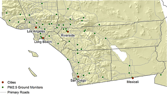
Figure 1. Study Domain and EPA Monitors. Study domain and underlying terrain for the area included in the current analysis. Location of EPA ground monitors are plotted, as well as major road networks.
Download figure:
Standard image High-resolution image2.2. Model input data
All 24-hour average PM2.5 and PM10 concentrations in 2012 were acquired from the EPA Air Quality System Data Mart (http://www.epa.gov/ttn/airs/aqsdatamart) [47]. A variable representing the ratio between PM2.5 and PM10 concentrations was calculated for use in the first stage of the modeling process to account for presence of dust and other coarse particles. To date, PM10 has yet to be regularly included in satellite-driven PM2.5 exposure models. Although MODIS AOD is generally most sensitive to smaller particles generally best characterized as PM2.5, coarse particles may also scatter or absorb light. As shown in this analysis, the southern California domain appears to have consistently high PM10 levels that warrant its inclusion as a predictor in our model to enhance PM2.5 predictions [48–51] Primary PM2.5 emissions (tons per year) and the number of major point sources for the study area were acquired from the EPA National Emissions Inventory and the total emissions were summed by grid cell. The aerosol optical depth (AOD) data at 1 km spatial resolution were extracted from the NASA MODIS Multi-Angle Implementation of Atmospheric Correction (MAIAC, MCD19A2) product (https://search.earthdata.nasa.gov/) [31, 52, 53]. The meteorological data such as air temperature, wind speed, and relative humidity were extracted from the North American Land Data Assimilation System Phase 2 (NLDAS-2) at 1/8-degree grid (∼ 12 km) resolution [54]. Planetary boundary layer height data were derived from the analysis fields of the North American Regional Reanalysis (NARR) at ∼ 32 km spatial resolution and 3-hour temporal frequency. NARR fields were spatially interpolated to the 1 km grid and then temporally disaggregated to the NLDAS hourly frequency [55].
Elevation was derived from the 3-arc-second (90-meter) Shuttle Radar Topography Mission (SRTM) dataset distributed by USGS Earth Resources Observation and Science (EROS) Data Center (https://www.usgs.gov/centers/eros). Additional land cover variables, including forest cover and impervious surfaces, were retrieved from the 2011 National Land Cover Database (NLCD, https://catalog.data.gov/dataset/usgs-2011-national-landcover). The spatial resolution of the NLCD coverage is 30 × 30 m2. Coverage maps were generated for forest pixels (pixels assigned 1 for forest and 0 for non-forest) and for percent imperviousness across the study area. Additional distance variables were included to account for potential effect modifiers unique to the region, including distance to the coastline and distance to Mexicali, Mexico. Road length data were obtained from ESRI StreetMap USA (Environmental Systems Research Institute, Inc. Redland, CA). The sum of the road segment lengths was determined in ArcGIS for each modeling grid cell. All model input data were mapped to the 1 km modeling grid using a spatial averaging procedure. Each PM2.5 monitoring site was matched to the nearest cell AOD, temperature, relative humidity, and wind speed. Land use variables were either averaged (forest cover and elevation) or summed (emissions, roads, point sources).
2.3. Modeling structure and cross validation
We calibrated the relationship between PM2.5 and AOD using a two-stage modeling framework, which allowed the relationship to vary in both space and time [33, 56, 57]. In the first stage, a linear mixed effects model (LME) was utilized with daily random slopes and intercepts for AOD, relative humidity, and wind speed. Since each of these variables are time varying, their inclusion as random effects aids in accounting for any temporal variation in the overall relationship between AOD and PM2.5. In addition to the random effects terms, the model included several fixed effects. Fixed effects in the model help to estimate the mean values and the included random effects help to account for daily variability in the relationship between dependent and independent variables. We considered multiple land use and meteorological predictors during the model selection process; however, we chose to eliminate some of the predictors from the final model due to lack of significance. The first stage of the model can be expressed by the following:
where PM2.5,sd represents ground-level PM2.5 concentrations in µg m−3 at each site (s) for each day (d); b0 and b0,d are respectively the fixed and random intercepts for the model; AODsd denotes the retrieved MAIAC AOD values at site s and day d with fixed and random day-specific slopes (b1 and b1,d); RelHumiditysd represents the measured relative humidity at site s and day d with fixed and random day-specific slopes (b2 and b2,d); WindSpeedsd is the average wind speed at site s and day d with fixed and random day-specific slopes (b3 and b3,d); PMRatiosd represents the ratio of PM2.5 to PM10 values; Tempsd is the average daily temperature at each site; %Cultivateds is the percentage cultivated to non-cultivated land at each site; Forests is an indicator variable denoting pixel forest cover; b0,d, b1,d, b2,d, b3,d are multi-variate normally distributed and Ψ represents the variance-covariance matrix for all random effects. The specific fixed effects for AOD, relative humidity, and wind speed aid in accounting for the average effects of these variables on the PM2.5 concentrations and the random effects are included to account for the daily variability between both the dependent and independent variables. Other potential confounders were assessed (boundary layer height, emission point sources, heat index, etc.). However, these did not influence the results and were omitted in the final model.
The purpose of the first stage of the model is to estimate the temporal PM2.5/AOD relationships with included effects of added covariates. However, we expect that the relationship will vary in space as well. To account for this potential additional variation, we added a second stage to the model utilizing geographically weighted regression (GWR) methods to create a continuous surface of estimates for parameters at each location. This incorporated using adaptive bandwidth selection methods in order to minimize the Akaike Information Criterion (AIC) value and aid in model selection. The GWR model structure can be expressed as:
where PM2.5.residuals represents the residual values from stage one of the model at site s for each day d; Coast.distance is the Euclidean distance calculated from each site s to the coast;, Mexicali.distance represents the distance from each site to Mexicali, Mexico; Elev is the elevation at each site s in meters;; and Roads is the sum of primary roads and highways within each grid cell; β0,s, refers to the location-specific intercept with β1,s, β2,s, β3,s, β4,s representing location-specific slopes for each of the parameters. The results from the second stage were then used as a calibration measure for the measurements obtained from the first stage of the model.
In order to assess the goodness of fit for the final model, we compared the outcome of the fitted model with the observed values using cross-validated coefficients of determination (CV R2) and root mean squared error (RMSE). A 10-fold cross-validation of the model was done by first randomly splitting the dataset into 10 equal subsets. The model was then run 10 times—each time one subset was kept in reserve as a test sample while the other 9 subsets were used to train the model. Since the calculation of the PMRatio variable included interpolation of PM10 observations, we chose to recalculate the PMRatio parameter for each of the 10 runs to avoid including information from the left-out subset. We then estimated predicted values for the remaining subset. Finally, the agreement between the predicted and observed values was then tested using the R2 and RMSE values and a comparison was made between the cross-validated model and the observations in order to assess agreement and/or potential over-fitting. Additionally, we conducted sensitivity analyses by running the full 2-stage model leaving out key parameters (AOD and PMRatio). We conducted all modeling and analyses in R 3.6.0 (2019) and ESRI ArcGIS® 10.6 (2018).
3. Results
3.1. Descriptive statistics
The annual mean PM2.5 concentration for all monitoring sites was 10.7 µg m−3, with maximum values as high as 78.8 µg m−3 present during the study period. The coverage for AOD values was 62% and overall mean AOD value was 0.08 with a maximum value of 2.96 during the study period. Maximum wind speeds reached 18.30 m s−1 with mean annual wind speeds measured at 4.78 m s−1. Additional parameters and corresponding mean, standard deviation, and range of the statistics are included in table 1.
Table 1. Descriptive Statistics of Considered Parameters.
| Variable | Mean | Std. Deviation | Minimum | Maximum |
|---|---|---|---|---|
| PM2.5 (µg m−3) | 10.77 | 6.30 | 0.00 | 78.78 |
| Aerosol Optical Depth | 0.08 | 0.07 | 0.01 | 2.96 |
| Boundary Layer Height (km) | 1.68 | 1.15 | 0.06 | 5.83 |
| Temperature (F) | 78.67 | 16.63 | 20.7 | 1.19 x10² |
| Relative Humidity (%) | 27.28 | 21.38 | 2.70 | 99.20 |
| Windspeed (m/s) | 4.78 | 1.84 | 0.60 | 18.30 |
| # of Point Sources | 0.04 | 0.34 | 0.00 | 36.00 |
| Average Emissions (tons per yr.) | 44.47 | 1.84x10² | 0.00 | 4.12x10⁵ |
| Primary Road Length (km) | 0.05 | 0.46 | 0.00 | 14.13 |
| Elevation (m) | 4.17x10² | 4.90x10² | −71.4 | 3.35x10³ |
| Impervious Land Cover (%) | 5.82 | 15.4 | 0.00 | 99.98 |
| Distance to Coast (km) | 1.05x10² | 84.62 | 0.00 | 3.22 x10² |
| Distance to Mexicali (km) | 2.01x10² | 98.35 | 0.00 | 4.25 x10² |
3.2. Model fitting
The model was fitted and the fixed effects estimated from the stage 1 linear mixed effects model are provided in table 2. The contributions of the intercept and parameters in the model are all significant at α = 0.05 level. The positive β values are indicative of a positive relationship between AOD, PM ratios, temperature, relative humidity, and cultivated land cover. Negative β values shown for wind speed and forest coverage suggest a negative relationship with PM2.5 concentrations. β values represent the change in the variable (keeping all others constant) that would increase the PM2.5 concentration by 1 µg m−3.
Table 2. First Stage Model Coefficients.
| Variable | β | p-value |
|---|---|---|
| Intercept | −7.03 | < 0.00 |
| AOD | 9.92 | <0.00 |
| PM Ratio | 14.80 | <0.00 |
| Temperature | 0.14 | <0.00 |
| Relative Humidity | 0.01 | 0.05 |
| Wind Speed | −0.18 | <0.00 |
| Forest Cover | −2.92 | < 0.00 |
| Cultivated Land Cover | 3.73 | < 0.00 |
3.3. Cross validation results
The first stage of the model has a CV R2 of 0.77 (model fitting R2 = 0.78) and CV RMSE of 2.41 µg m−3 (original model RMSE = 2.38 µg m−3). Compared with the original model, the results from the CV suggest slight model over-fitting as shown by the changes in statistical measures of R2 and RMSE. The second stage of the model (or full model) incorporates the first stage and GWR methods and resulted in a CV R2 increase to 0.80 (original model R2 = 0.85) and a change in CV RMSE to 2.25 µg m−3 (original model RMSE = 1.96). As shown in these validation results, the second stage of the model improved the overall prediction performance with a CV R2 increase of 0.03 from the first stage to the second stage of the model and a 0.16 µg m−3 decreased CV RMSE between the two stages. This improvement in accuracy could indicate the ability of the GWR methods for capturing more of the spatial variation in the data than is possible with the LME stage alone. These results suggest that adding a second stage to account for spatial as well as temporal variability can substantially improve model accuracy.
3.4. PM2.5 estimations
Annual mean PM2.5 at ground stations alone and across the entire domain based on inverse distance weighting can be seen in figure 2. This comparison shows an increased coverage of exposure with this simple interpolation technique; however, this method lacks the spatial detail necessary to be confident in the estimated exposures located at greater distances from monitoring stations. For example, with the simple interpolation method, major differences in PM2.5 concentrations can be found, such as those near the Mexican border. The annual mean PM2.5 estimated from model fitting for the 1 km × 1 km grid is shown in figure 3, with figure 3(A) showing results of the analysis including the PMRatio parameter and figure 3(B) showing results without including PMRatio. As seen in figure 3(A), annual averaged PM2.5 tends to result in high concentrations seen in population centers, along some major highways, and in valleys and canyons. Estimated concentrations align closely with the topography of the surrounding areas (see figure 1). In the Los Angeles area, lower concentrations of PM2.5 are seen on the coast, with increasing concentrations to inland population centers (i.e. Riverside). In San Diego, the same trends occur, but with higher coastal PM2.5 than Los Angeles. The Imperial Valley area is subject to higher concentrations due to transport from Mexico, major highways, high airborne dust, and surrounding topography.
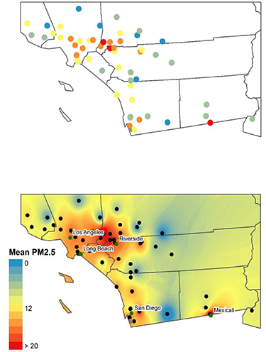
Figure 2. Interpolation of EPA Monitor Mean Annual PM2.5 Concentrations. Using ArcGIS, the top plot represents interpolation at each EPA ground monitor using nearest neighbor averaging. The bottom plot shows the use of interpolation across the domain surface using inverse distance weighting at each EPA ground monitor.
Download figure:
Standard image High-resolution image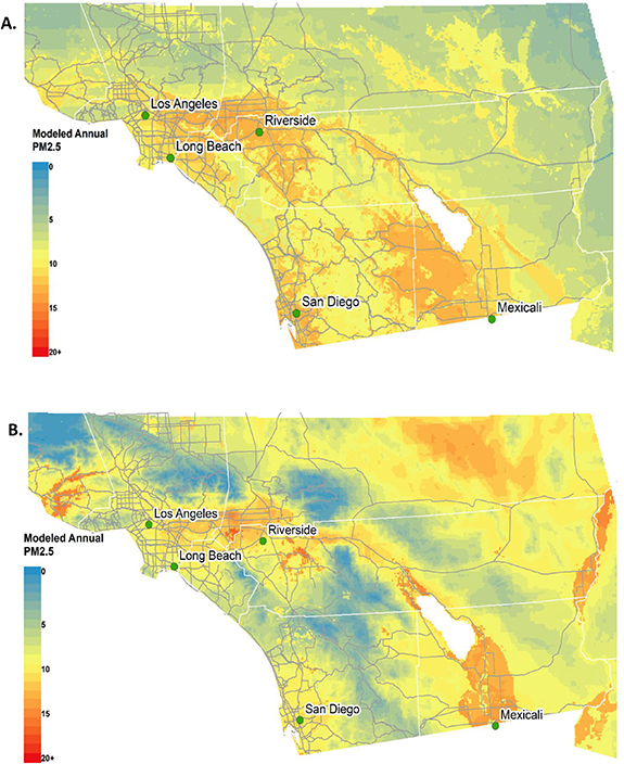
Figure 3. Predicted Annual Average PM2.5 Concentrations Utilizing PM2.5/PM10 Ratios. Predicted annual average PM2.5 concentrations using two-stage linear mixed effects and geographically weighted regression models at a resolution of 1 km × 1 km. Figure 3(A) depicts the model without inclusion of the PMRatio parameter. Figure 3(B) represents the full model incorporating the PMRatio variable.
Download figure:
Standard image High-resolution image3.5. Importance of PM2.5/PM10 relationship in Southern California
During the process of model fitting, it was found that the presence of dust (or larger sizes of PM) in the troposphere is an integral part of the AOD-PM2.5 relationship in southern California (β = 14.79, p ≤ 0.00). We accounted for this by adding a model parameter representing the observed PM2.5 divided by the monthly mean PM10 for each site. The pattern of PM2.5 to PM10 ratio is shown by the location of EPA monitoring stations in Supplemental figure 1. There was a strong positive correlation between PMRatio and observed PM2.5 (r = 0.7) and a weak negative association with observed PM10 (r = −0.4, see Supplemental table 1 for complete correlation results). The importance of this parameter was also tested by running the model with and without the PM2.5 to PM10 ratio. In figure 3(A), the ratio of PM2.5 to PM10 was not included in the model, resulting in full model CV R2 was 0.70 with a CV RMSE of 2.81 µg m−3. However, with the inclusion of this ratio parameter in figure 3(B), accounting for larger particles significantly improved the model performance, resulting in the CV R2 = 0.80 and a RMSE = 2.25. Detailed results comparing the full model with models without the PM2.5 to PM10 ratio and without AOD can be seen in Supplemental table 1, and temporal patterns of monthly AOD and the PM2.5 to PM10 ratio are shown in Supplemental figure 2. Notably, the spatial patterns of the PMRatio variable can change greatly from monitor to monitor—even between monitors relatively close in proximity to one another. This is likely due to the shorter airborne residence time of larger particles, which vary greatly depending on current conditions.
Seasonality of PM2.5
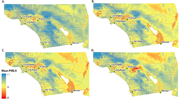
Figures 4(A)–(D) illustrates the seasonal patterns of PM2.5 concentrations in the study domain. The mean predicted concentrations varied by quarter with a mean of 4.24 µg m−3 in the first quarter, 6.77 µg m−3 in the second, 7.37 µg m−3 in the third, and 7.75 µg m−3 in the final quarter. Precipitation during California's rainy season (∼ October-April) can contribute to low PM2.5 concentrations, as seen in the first and second quarter mean results. These means also follow the general patterns of PM2.5 concentrations and temperature. Maximum concentrations were found in the final quarter (max = 22.77 µg m−3) and we see a decrease in first and second quarterly overall PM2.5 compared to later levels. However, concentrations surrounding populated areas may still be pronounced.
Figure 4.. Quarterly Predicted Average PM2.5. Maps depicting the 4 calendar quarters in southern California and subsequent mean PM2.5 concentrations. (A) January, February, March 2012, (B) April, May June 2012, (C) July, August, September 2012, (D) October, November, December 2012. Lower concentrations tend to be seen in the cooler months with increasing means throughout the year.
Download figure:
Standard image High-resolution image
4. Discussion
In this study, we sought to identify parameters important for modeling PM2.5 levels in the Southern California region. Given the potential differences between regions, it is important to characterize the factors that contribute to PM2.5 concentrations in multiple regions. Furthermore, understanding these region-specific associations is especially important in the Western US, where several cities experience some of the worst air quality in the country. Thus, we opted for a two-stage statistical model that allowed us to evaluate the relative importance of model covariates. Based on previous literature, several factors may contribute to overall PM2.5 model performance [1, 21, 23, 24, 27, 28, 33, 58–61]. This is especially true if these parameters differ by region. For instance, low wind speeds have been shown to contribute to PM2.5 concentrations [62–64]. Wind speeds can also vary greatly between regions; with areas like California reaching lowest wind speeds in the fall and winter months [65, 66]. Conversely, regions such as the southeastern US experience lower mean wind speeds in the summer—which could affect the seasonality of PM2.5 [66]. In terms of relative humidity, a similar pattern emerges with annual relative humidity overall decreasing annually for the western US while annual increases are evident in southeastern states [65]. Temperature is also spatially dependent. This is evident in a general increase in temperatures across the west, southwest, south, and northeast regions of the US, with states in the north central region exhibiting temperature decreases [65].
In light of these inherent meteorological differences and in an effort to identify which parameters are most important for southern California, we adopt a simple two-stage model approach. Of all possible parameters, we chose to assess AOD, temperature, wind speed, relative humidity, boundary layer height, point sources, annual emissions, road length, impervious land cover and distances to the coast and Mexicali, Mexico. AOD is an optical measure of the abundance of fine particles in the air, and significant positive associations have been shown between PM2.5 and AOD. However, AOD coverage can vary between regions and could contribute to differences found in β-values and model performance. Secondly, temperature has also been shown to have a positive relationship with PM concentrations in the troposphere. Our results follow this trend, showing a significant positive association with temperature. Associations between PM2.5 and other covariates are also evident in our model results, including relative humidity, wind speed, forest cover, and cultivated land. The small positive beta value found for relative humidity suggests a slight positive relationship with PM concentrations and humidity—which can greatly differ from one location to another. An additional positive association was found between cultivated land and PM2.5. Since cultivated land is defined as land in use for farming (including land that is being actively tilled), this parameter may intuitively account for a portion of the PM concentrations in the air. Negative associations were shown for both wind speed and forest cover, as one might expect. A negative association for wind speed may be explained by a diluting effect on PM concentrations—especially at higher wind speeds. These higher wind speeds can cause rapid dispersion of particles and decrease concentrations that may otherwise be found at specific locations. Forest cover can also exhibit a negative relationship with PM concentration—which may be due to the settling and/or absorption of PM due to presence of trees. The boundary layer height (BLH), often a strong predictor in PM2.5 models, was not included in our final model. Generally, higher BLH is associated with lower PM2.5 concentrations as a result of greater vertical mixing. However, if the BLH variable has little variation or an irregular distribution, this can contribute to less importance seen in the model diagnostics. This is, in fact, the case in our modeling structure (as shown in Supplemental figure 3), where BLH has a bimodal distribution. This irregular distribution is likely due to terrain variations in our study domain ranging from coastal regions to inland mountains.
While multiple national-level studies exist, it is clear that many of these associations could be region-specific. For example, Lee et al (2016), a satellite/ground-based approach in the southeastern US resulted in relatively high R2 values, with mean CV R2 estimates > 0.7. Similar results were found both with and without a PM10 parameter [36]. However, in other publications, similar models in the western US and California show lower performance. For instance, Franklin et al (2017) showed that a spatio-temporal model including similar parameters used in our study resulted in a CV R2 of 0.51 without accounting for PM10 [67]. While there could be multiple explanations for the differing model structures for each region, perhaps the most significant predictive variable in our model was the presence of airborne dust. As seen in other parameters, dust seems to be a more important factor in the Southwest US than in other areas [68]. This can be seen when models are run both with and without accounting for airborne dust, with significantly higher R2 values found in when including a dust component. Thus, we sought to create a variable that would help to control for the effects of airborne dust by calculating the ratio of PM2.5 to PM10 particles. In doing so, we utilized the PM2.5/PM10 ratio as a proxy for dust, which greatly enhanced our model results. Another approach could include applying the current model structure to other regions to serve as an additional source of model validation. However, since our intention was an exploratory investigation concerning the characteristics of the US west coast, this approach was not applicable.As mentioned, the fall months in this area experienced the maximum PM2.5 concentrations. This is likely due to a phenomenon that occurs in the late fall in the southern California region called the Santa Ana winds. Santa Ana winds are foehn winds responsible for some of the largest and most devastating wildfires in California history [69]. These winds originate from high-pressure inland systems that flow outward to the west coast. Typically, the fuel sources during these months are extremely dry and these prevailing winds bring higher temperatures and lower humidity to the surrounding atmosphere. Thus, not only do the Santa Ana winds create better conditions for fire ignition, their high speeds also provide a driving force for dust generation and entrainment. Hence, the occurrence of the Santa Ana's may be associated with increased PM concentrations in the fall months due to prolonged fire seasons driven by these seasonal winds [69–73]. While our model is not able to capture smoke-specific PM2.5, we were able to show an average increase in PM2.5/PM10 ratio during the fall months. Wildfire smoke is generally composed of fine mode particles and higher PM2.5/PM10 ratios are indicative of higher amounts of smaller airborne particulates (see supplemental figure 2) (available online at stacks.iop.org/ERL/15/094004/mmedia) [74, 75]. Thus, while particle speciation was beyond the scope of this study, higher PM2.5/PM10 ratios during the fall months may suggest higher wildfire activity.
Our study adds significantly to the current body of research on the subject of using remote sensing data to achieve better exposure data—especially in regions with higher dust concentrations. To our knowledge, this study is the first to utilize high-resolution MAIAC data to estimate PM2.5 concentrations in southern California—giving much needed information on a highly populated area with potential health risks due to elevated pollutant exposures. As reported above, a key finding of this study is the importance of accounting for the contribution of coarse particles to AOD. Without a specific fine mode fraction parameter from MAIAC, we included the ratio between PM2.5 and PM10 in the first stage of the model. Our results add meaningful insight into the way to improve model performance when study domains include areas with high air-dust content. Due to the large number of ground monitors in the southern California region, we were able to develop an exposure model with consistent model performance. While multiple years of data are needed to better represent transient PM2.5 emissions sources such as wildfires, this was not the focus of the current study. However, our finding that the influence of PM10 to AOD needs to be considered suggests that coarse particles can significantly affect the overall aerosol light extinction in California, therefore modify the association between satellite AOD and ground level PM2.5 concentrations. Thus, with PMRatio as a model predictor, we believe our model is generalizable to other dust-prone areas in California. We acknowledge that there are areas where AOD was missing due to cloud cover or other surface albedo issues (AOD coverage = 62%). While techniques for AOD gap-filling have been used elsewhere, it was not the main goal of this study. Thus, simpler gap-filling methods were used. Our intent was to provide MAIAC AOD as an enhancement to ground PM2.5 estimations over previous, lower resolution products in the area of southern California.
5. Conclusion
Using southern California as an example, this paper investigated the feasibility of using the high-resolution MAIAC AOD to estimate ground-level PM2.5 concentrations in the Western US. While the two-stage model structure has been used in many applications, it revealed the importance of considering larger particles in airborne dust-prone areas and may be an underlying cause for previous poor model performances. Further research may be needed to explore other possible indicators of the coarse particle contribution to AOD. Additional steps might include more sophisticated gap-filling techniques and investigations into additional land use, population, or meteorological parameters that may significantly affect the PM2.5-AOD relationship in southern California.
Acknowledgments
The work of J. Bi, J. Stowell, and Y. Liu was supported by the NASA Applied Sciences Program (Grant # NNX16AQ28Q and 80NSSC19K0191) and the MISR science team at the JPL, California Institute of Technology, led by D. Diner (subcontract # 1363692).
Declaration of Competing Financial Interests
The authors declare they have no actual or potential competing financial interests.
Data Availability
The data that support the findings of this study are available from the corresponding author upon reasonable request.