Article

An Optimal Day-Ahead Thermal Generation Scheduling Method to Enhance Total Transfer Capability for the Sending-Side System with Large-Scale Wind Power Integration

1
State Key Laboratory of Alternate Electrical Power System with Renewable Energy Sources, North China Electric Power University, Beijing 102206, China
2
State Grid Corporation of Gansu Province, Lanzhou 730000, China
*
Author to whom correspondence should be addressed.
Energies 2020, 13(9), 2375; https://doi.org/10.3390/en13092375
Submission received: 11 April 2020 / Revised: 4 May 2020 / Accepted: 6 May 2020 / Published: 9 May 2020

Abstract

:
The rapidly increasing penetration of wind power into sending-side systems makes the wind power curtailment problem more severe. Enhancing the total transfer capability (TTC) of the transmission channel allows more wind power to be delivered to the load center; therefore, the curtailed wind power can be reduced. In this paper, a new method is proposed to enhance TTC, which works by optimizing the day-ahead thermal generation schedules. First, the impact of thermal generation plant/unit commitment on TTC is analyzed. Based on this, the day-ahead thermal generation scheduling rules to enhance TTC are proposed herein, and the corresponding optimization models are established and solved. Then, the optimal day-ahead thermal generation scheduling method to enhance TTC is formed. The proposed method was validated on the large-scale wind power base sending-side system in Gansu Province in China; the results indicate that the proposed method can significantly enhance TTC, and therefore, reduce the curtailed wind power.

Graphical Abstract

1. Introduction

Large-scale wind power bases are mostly located in the areas with rich wind energy and far from the load center. Because of the small capacity of local load, a vast amount of wind power needs to be delivered through a transmission channel to the load center. Wind power is highly intermittent; during the periods of large availability of wind energy, the lack of consumption space in local areas and the restriction of total transfer capability (TTC) of the transmission channel are two main reasons for wind power curtailment.
Many relevant studies focus on expanding consumption space for wind power in the local areas of large-scale wind power bases. A pair of studies [1,2] suggest that the curtailed wind power could be consumed by the energy-intensive load, which is located close to the large-scale wind power base and has better regulation flexibility than residential load. Two papers [3,4] studied the potential of deep peak regulation of thermal generation units and proposed a wind-thermal peak regulation trading mechanism to help consume wind power. However, through economic analysis [5] revealed that blindly reducing the wind power curtailment using the supply side and demand side resources may not be cost-effective. References [6,7] show that a wind power generation system equipped with energy storage can smooth the fluctuation of wind power, but it needs a fairly large investment. Using the methods given above, during the periods of large availability of wind energy, wind power can be further consumed in the local areas by regulating energy-intensive load upward, regulating the output of thermal generation units deep downward and storing wind energy.
The above studies have provided methods that can effectively improve the wind power curtailment situation. However, the installed capacity of wind power in a large-scale wind power base is far too large; the curtailed wind power cannot be fully consumed through the above-mentioned methods. Delivering wind power through the transmission channel to the load center is still an important way to consume large-scale wind power. Reference [8] shows that the flexible demand response in the load center can shift the load to wind power peak periods, which enables the receiving-side system to spare more available consumption space for wind power. However, large-scale wind power delivered through the transmission channel makes the transmission channel vulnerable [9]. Therefore, enhancing TTC and making full use of the transmission channel is of great significance for wind power consumption.
TTC of the transmission channel is usually limited by its transient stability-constrained total transfer capability (still referred to as TTC) [10], so TTC can be enhanced by improving system transient stability. Some studies have found that flexible AC transmission system (FACTS) devices could be utilized to improve transient stability besides their main function of controlling power flow [11,12,13,14]. FACTS devices including the unified power flow controller (UPFC) and the thyristor switched series capacitor (TSSC) use silicon controlled rectifiers (SCRs) instead of traditional mechanical switches. The development of silicon-coated gold nanoparticle technology enables FACTS devices to achieve super-resolution and quicker adjustment according to the system instructions [15,16]. Reference [11] modulates the active power and reactive power using UPFC to improve the first swing stability and achieves enhancing TTC of long-distance transmission lines. The authors of [12] designed a power oscillation damping controller which enables TSSC to have continuous reactance, and by decreasing the reactance between the sending and receiving ends, TTC can be enhanced. However, the main function of FACTS devices is not to improve the system’s transient stability; what is more, for the systems that do not have FACTS devices, installing them requires additional costs.
Transient stability analysis shows that some electrical parameters, such as the inertia constant and grid reactance, have great impacts on system transient stability [17]. Due to the differences in the electrical parameters of thermal generation units, system electrical parameters and TTC change with thermal generation unit commitment. For a system with large-scale wind power integration, day-ahead thermal generation scheduling is necessarily made to ensure power balance, mostly with the objective of minimizing the generation cost, sometimes considering the objectives of maximizing the reliability of the power system and minimizing the emission [18,19]. However, no previous work on enhancing TTC by optimizing thermal generation schedules has been reported.
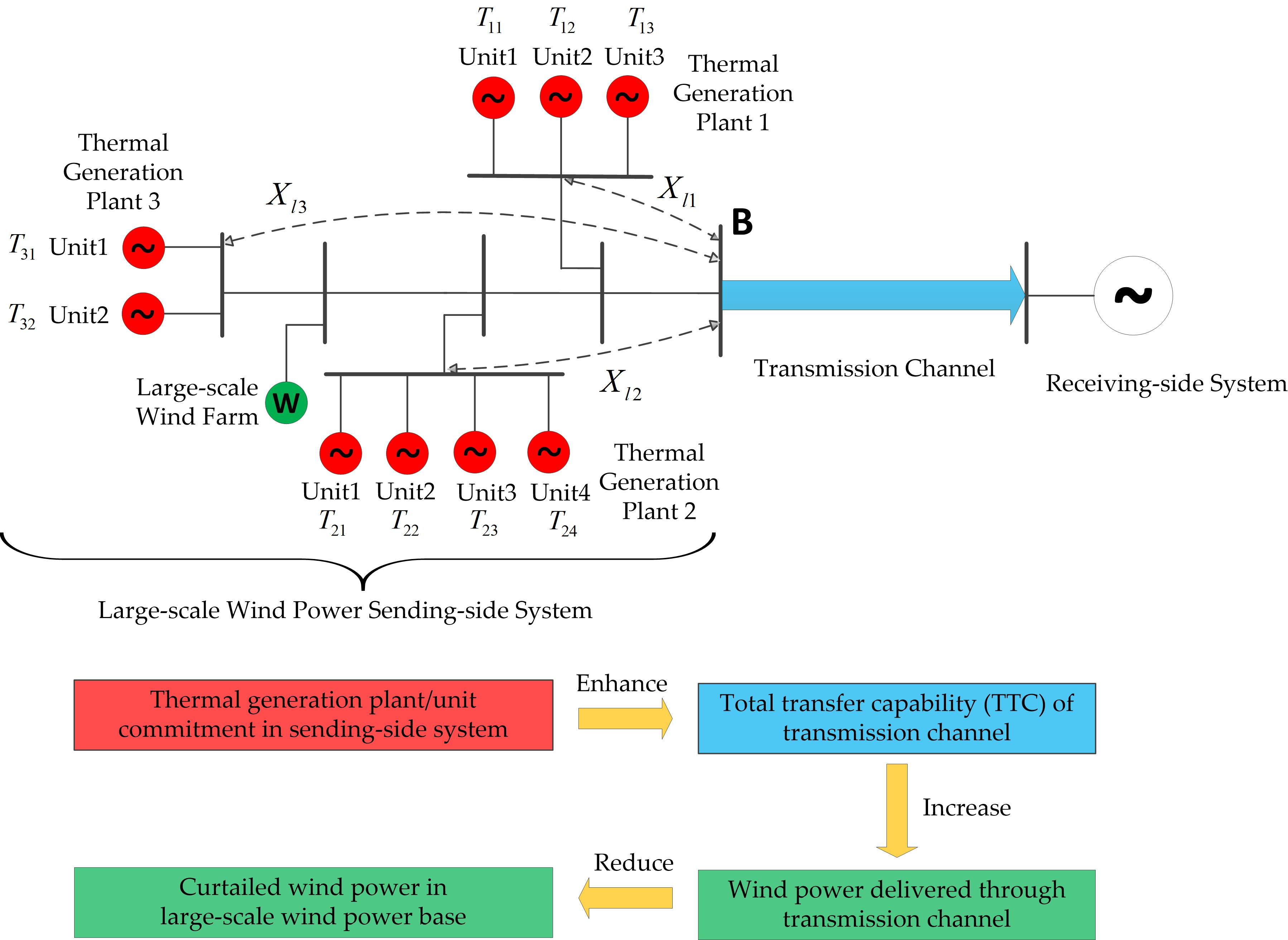
This paper presents a new method with which to enhance TTC based on the existing grid structure, which is by optimizing the day-ahead thermal generation schedules, and it can help reduce curtailed wind power for the sending-side system with large-scale wind power integration. This method is especially suitable for the sending-side system with thermal generation plants and large-scale wind power integration and the transmission channel in its existing grid structure, which is the common structure of large-scale wind power bases. The resources that are used in this method only involve the existing thermal generation plants, and it requires no further installment of devices. The main contributions are as follows:
  • The mechanism of the impact of thermal generation plant/unit commitment on TTC is revealed.
  • TTC is enhanced by optimizing the day-ahead thermal generation schedules, requiring no investment in installing additional devices. With the enhanced TTC, more wind power is allowed to be delivered through the transmission channel to the load center; therefore, the curtailed wind power is reduced.
The rest of the paper is organized as follows. In Section 2 and Section 3, the impact of enhancing TTC on reducing curtailed wind power and the mechanism of the impact of thermal generation plant/unit commitment on TTC are analyzed. In Section 4, the optimal day-ahead thermal generation scheduling method to enhance TTC is proposed. In Section 5, the case analysis is presented. Finally, the conclusions are given in Section 6.

2. The Impact of Enhancing TTC on Reducing Curtailed Wind Power

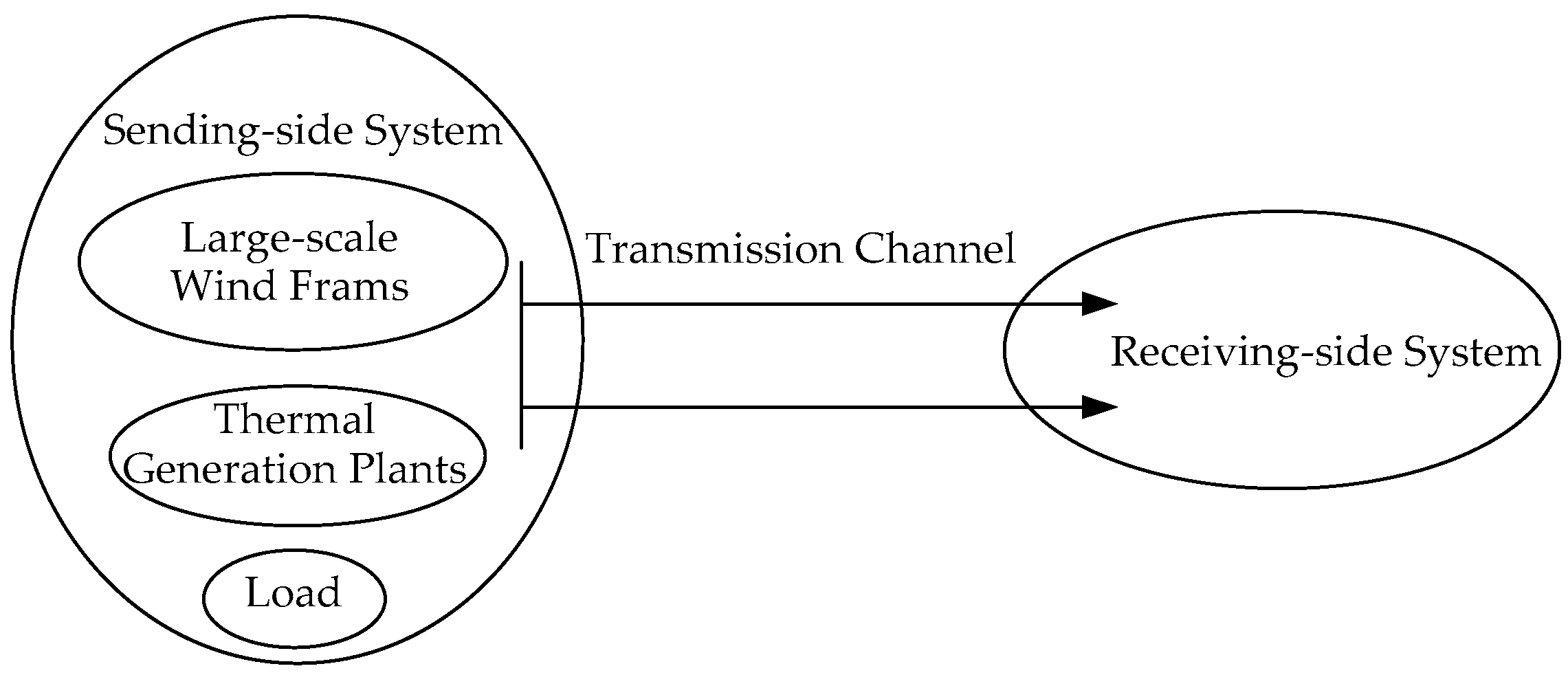
Figure 1 shows a schematic diagram of a sending-side system with large-scale wind power integration, a receiving-side system and the transmission channel between them. Assuming that during the periods of large availability of wind energy, wind power is curtailed, the impact of enhancing TTC on reducing curtailed wind power is analyzed below.
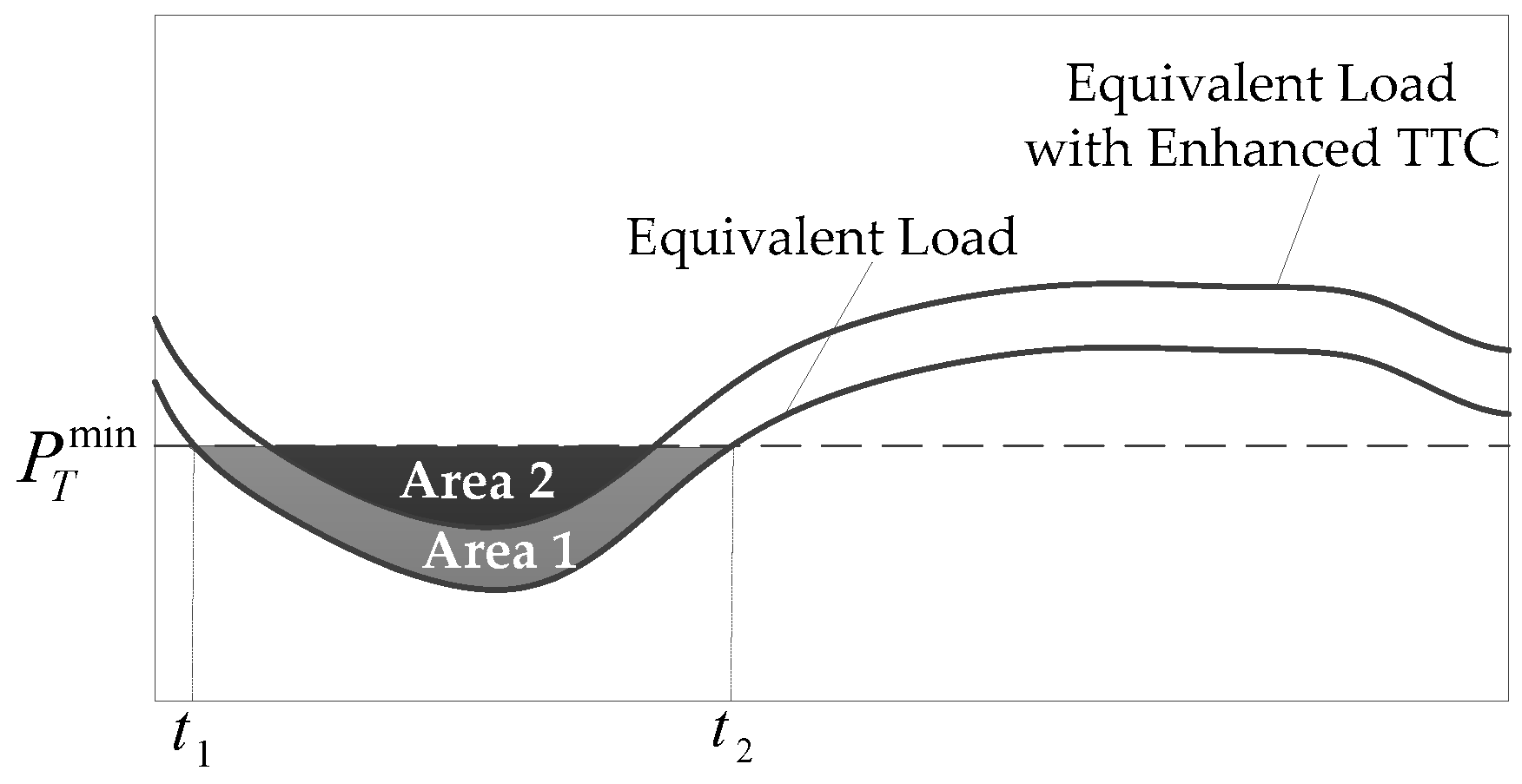
For the sending-side system, the wind power output is regarded as a negative load, and the power delivered through the transmission channel is regarded as a positive load. The equivalent load in the sending-side system is as follows:
P E L = P S L + P D P W
where P S L is the total load in the sending-side system, P D is the power delivered through the transmission channel and P W is the wind power output.
The equivalent load is balanced with the thermal generation in the sending-side system as follows:
P T P E L = 0
where P T is the thermal generation in the sending-side system.
During the periods of large availability of wind energy, the power delivered through the transmission channel reaches TTC, and if the minimum allowable thermal generation P T m i n is greater than the equivalent load P E L , wind power needs to be curtailed, and the curtailed wind power is the sum of Area 1 and Area 2 during periods t 1 ~ t 2 in Figure 2.
If TTC is enhanced, the power delivered through the transmission channel P D can be increased; according to Equation (1), the equivalent load P E L is increased accordingly. Therefore, the curtailed wind power reduces from the sum of Area 1 and Area 2 to Area 2 in Figure 2.

3. The Impact of Thermal Generation Plant/Unit Commitment on TTC

The TTC of the transmission channel is usually limited by its transient, stability-constrained total transfer capability, which is considered as a security constraint while making generation schedules. In fact, due to the differences of thermal generation plants and units in terms of their electrical parameters and their electrical distances from the transmission channel, thermal generation plant/unit commitment has a great impact on TTC.
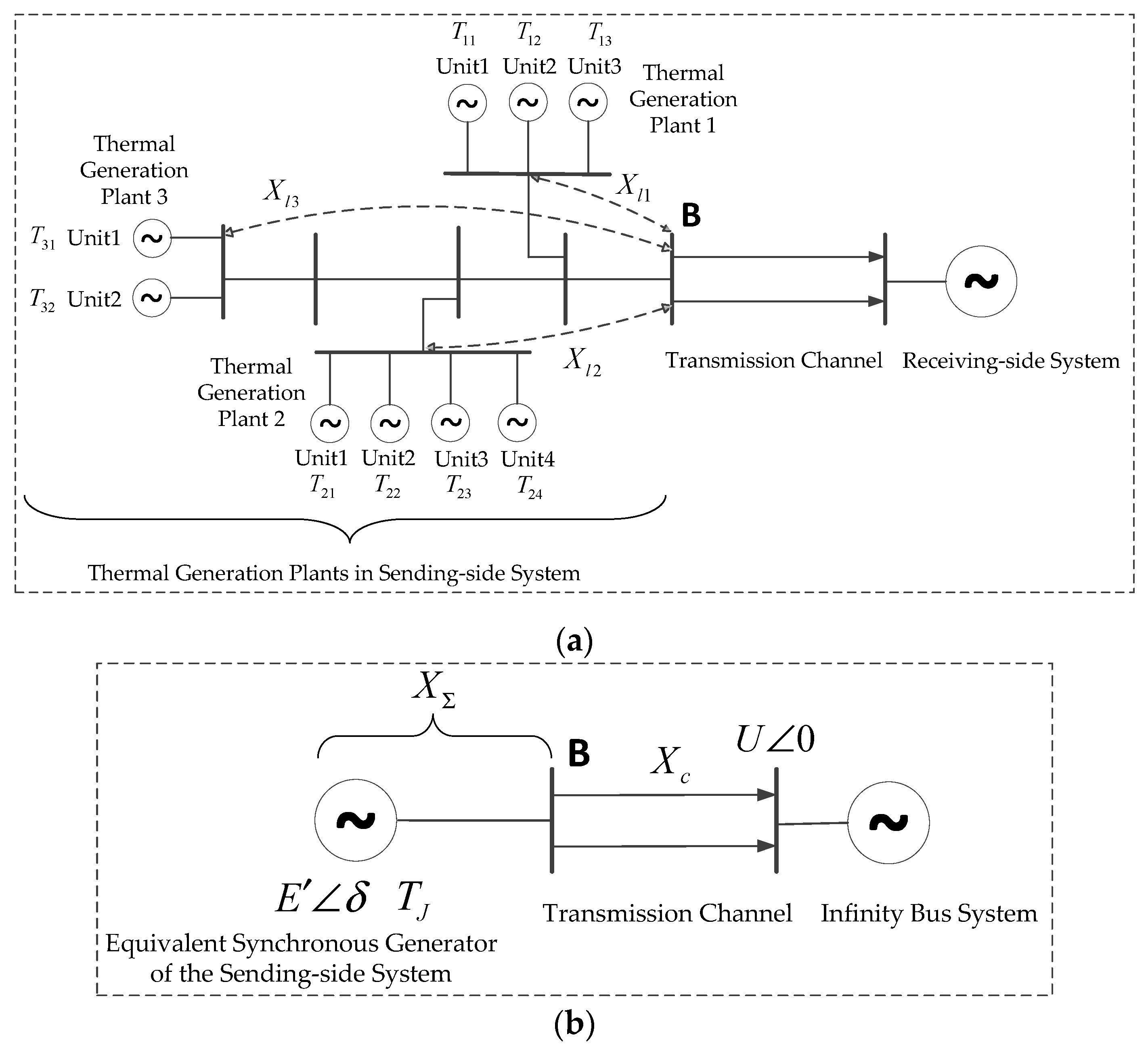
As shown in Figure 3, for a multi-generator sending-side system, while analyzing the impact of thermal generation plant/unit commitment on TTC, the wind farms and load are omitted. The online thermal generation units in the sending-side system are equivalent to one synchronous generator, and the receiving-side system is equivalent to an infinity bus system.
Under the condition that the system is able to stay transiently stable after a fault occurs, the maximum steady state power that can be delivered through the transmission channel in Figure 3b represents TTC (it is not the actual TTC, but it can be used for qualitatively analyzing the impact of thermal generation plant/unit commitment on TTC). The system transient stability is evaluated by the stability of the synchronous generator rotor angle in the first swing after a fault occurs. The rotor motion equation of the equivalent synchronous generator of the sending-side system is shown in Equations (3) and (4):
δ ¨ = d 2 δ ( t ) d t 2 = 1 T J ( P m P e )
P e = E U X Σ + X c s i n δ ( t ) = P e m a x s i n δ ( t )
where δ , E , T J , P m , P e are the rotor angle, internal voltage, inertia constant, mechanical and electrical power of the equivalent synchronous generator of the sending-side system, respectively. δ ¨ is the acceleration of δ . P e m a x is the maximum of P e . P m equals the steady state value of P e , and it represents the steady state power delivered through the transmission channel. U is the magnitude of the infinity bus voltage, and the phase angle of the infinity bus voltage remains 0. Reactance X Σ is the equivalent electrical distance between the transmission channel and the equivalent synchronous generator of the sending-side system. X c is the reactance of the transmission channel.
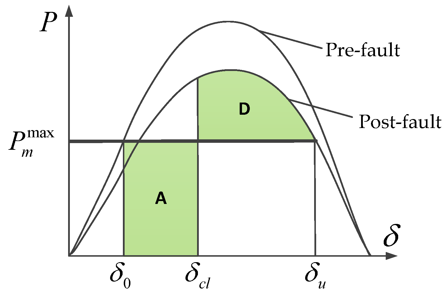
According to equal area criterion [20], if the rotor’s acceleration area A during the fault is equal to its maximum possible deceleration area D after the fault is removed, the system is in the transient stability critical state, and P m reaches its maximum value P m m a x which represents TTC, as shown in Figure 4.
According to Equations (3) and (4), X Σ and T J are both important factors in the system’s transient stability evaluation, so they have an impact on TTC. Due to the differences of thermal generation plants and units in their electrical distances from the transmission channel and their inertia constants, as shown in Figure 3a, thermal generation plant/unit commitment has a great impact on X Σ and T J , and therefore, on TTC, and the detailed analysis is as follows.

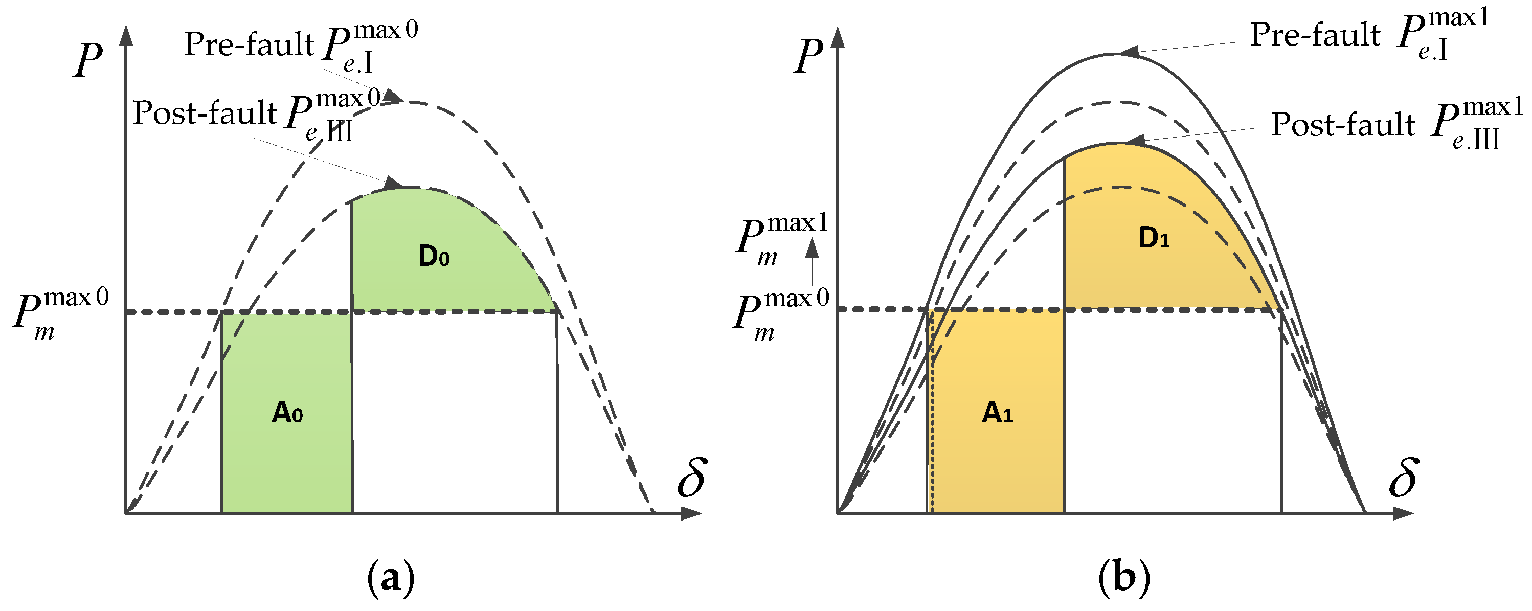
3.1. The Impacts of Thermal Generation Plant Commitment on X Σ and TTC

The impact of X Σ on TTC is analyzed through Figure 5. If X Σ decreases from X Σ 0 in Figure 5a to X Σ 1 in Figure 5b, according to Equation (4), P e m a x will increase from P e m a x 0 to P e m a x 1 (superscript “0” and “1” correspond to Figure 5a,b, respectively). TTC in Figure 5a is P m m a x 0 , and assuming the power delivered through the transmission channel in Figure 5b remains P m m a x 0 , it can be seen that A 1 A 0 and D 1 > D 0 , which means the system in Figure 5b has not reached the transient stability critical state, and there is still space for P m to increase; therefore, P m m a x 1 > P m m a x 0 . In conclusion, TTC increases with the decrease of X Σ .
For the three thermal generation plants in the sending-side system in Figure 3a, assuming X l 1 < X l 2 < X l 3 and ignoring the influences of other parameters, if only two thermal generation plants need to be online, then the plant commitment of Plant 1 and Plant 2 can obtain the minimum X Σ and the maximum TTC.

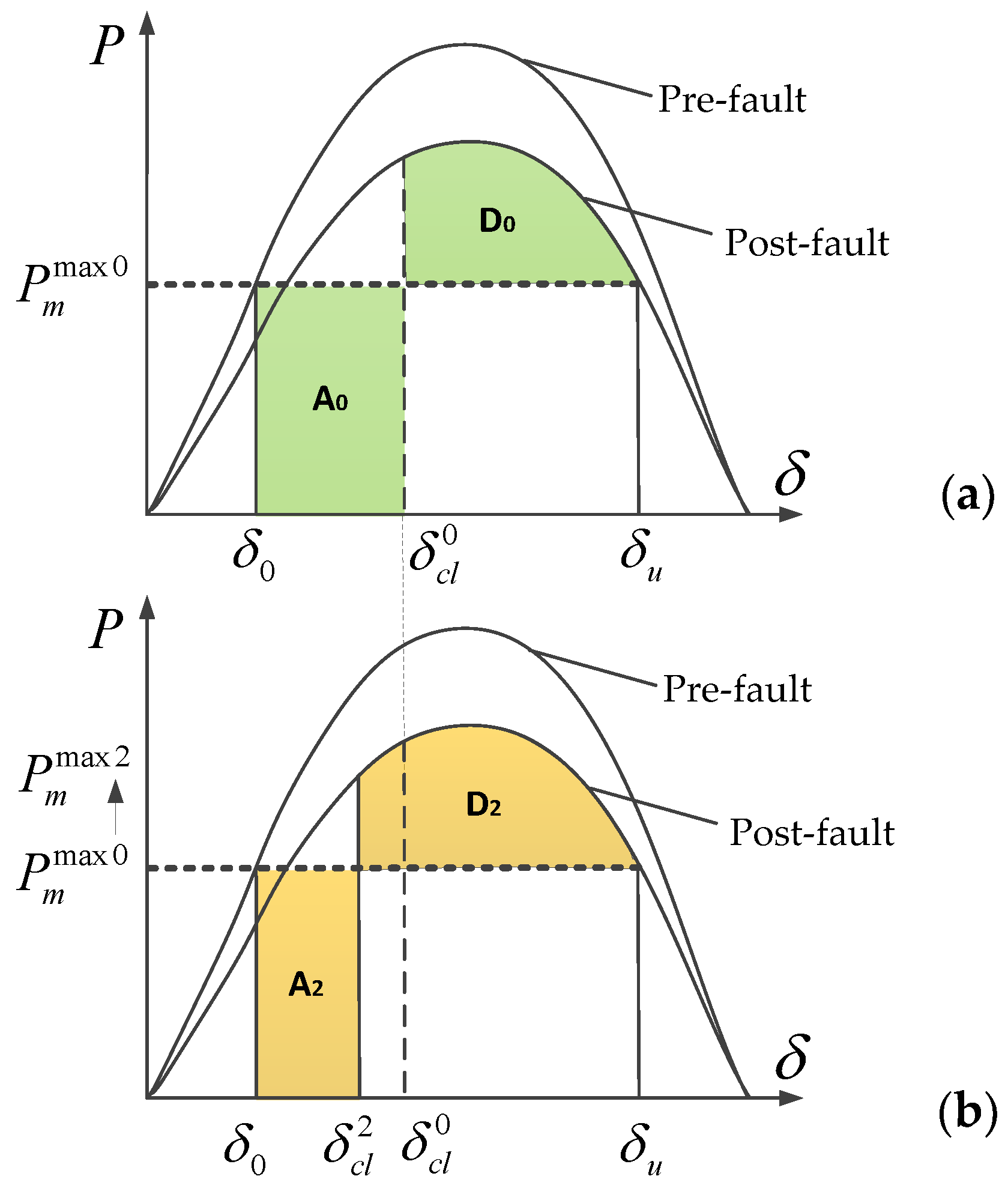
3.2. The Impacts of Thermal Generation Unit Commitment on T J and TTC

The impact of T J on TTC is analyzed through Figure 6. If T J increases from T J 0 in Figure 6a to T J 2 in Figure 6b, according to Equation (3), δ ¨ will decrease, so the fault removal rotor angle δ c l will decrease from δ c l 0 to δ c l 2 (superscript “0” and “2” correspond to Figure 6a,b, respectively). TTC in Figure 6a is P m m a x 0 , and assuming the power delivered through the transmission channel in Figure 6b remains P m m a x 0 , it can be seen that A 2 < A 0 and D 2 > D 0 , which means the system in Figure 6b has not reached the transient stability critical state, and there is still space for P m to increase; therefore, P m m a x 2 > P m m a x 0 . In conclusion, TTC increases with T J .
For each thermal generation plant that is scheduled to be online, its equivalent inertia constant changes with the thermal generation unit commitment inside the plant. TTC increases with the equivalent inertia constant of each online thermal generation plant.

4. Optimal Day-Ahead Thermal Generation Scheduling Method to Enhance TTC

4.1. Day-Ahead Thermal Generation Scheduling Rules

Based on the impact of thermal generation plant/unit commitment on TTC, the day-ahead thermal generation scheduling rules to enhance TTC are proposed as follows:
Rule 1: For thermal generation plant commitment, the plants with shorter electrical distances from the transmission channel take priority.
Rule 2: For thermal generation unit commitment inside the thermal generation plant which is scheduled to be online, the units with bigger inertia constants and lesser generation costs take priority.
Rule 3: According to the above rules, optimize the day-ahead thermal generation schedules to enhance TTC, and then increase wind power output based on the enhanced TTC to reduce curtailed wind power.

4.2. Day-Ahead Thermal Generation Plant Commitment Optimization

4.2.1. Day-Ahead Thermal Generation Plant Commitment Optimization Model

According to Rule 1, the day-ahead thermal generation plant commitment optimization model is established as follows:
  • Objective
    The objective is to obtain the minimum equivalent electrical distance between the transmission channel and the equivalent synchronous generator of the sending-side system.
    min   X Σ ( U P )
    where U P = ( U P 1 , , U P N P ) is the vector of the online/offline state of the thermal generation plants and N P is the number of the thermal generation plants in the sending-side system. If the i th thermal generation plant is online, then U P i = 1 ; otherwise, U P i = 0 ; and once the state is settled, it does not change in one day. X Σ is the function of U P , and it is calculated using the Gaussian elimination equivalent method as follows:
    X Σ = Im ( 1 Y P B T E Y P B T Y P P 1 Y P B )
    where Im ( ) is the imaginary part of . Y P P is the thermal generation plant’s node admittance matrix in the sending-side system; B is the border node in the sending-side that the transmission channel connects to, as shown in Figure 3. Y P B is the column vector of mutual admittance between node B and the nodes in the sending-side system. E is a unit column vector with the same dimensions as Y P B .
  • Constraint:
    The online thermal generation plants should be able to supply enough generation for the equivalent load and spare an appropriate amount of backup and reserve capacity.
    i = 1 N P U P i P p i m a x P E L . f o r c a s t m a x + P B
    where P P i m a x is the maximum allowable output of the i th thermal generation plant. P E L . f o r c a s t m a x is the maximum equivalent load forecast; P E L . f o r c a s t m a x = max t T d P E L . f o r c a s t t ; T d is the set of day-head scheduling periods, and the equivalent load forecast P E L . f o r c a s t t can be obtained from Equation (1), with the known total load forecast and wind power forecast in the sending-side system and the initial scheduled power delivered through the transmission channel. P B is the backup and reserve capacity, and each online thermal generation plant should at least have one spare generation unit for emergency.
    After the thermal generation plant commitment is settled, the generation schedule for each online thermal generation plant is in proportion to its maximum allowable output.
    P P i t = U P i P P i m a x i = 1 N P U P i P P i m a x P E L . f o r c a s t t
    where P P i t is the generation schedule of the i th thermal generation plant in period t .

4.2.2. Solution Algorithm

The day-ahead thermal generation plant commitment optimization model is a 0–1 optimization problem, and the number of thermal generation plants in the large-scale wind power base sending-side system is finite and relatively small; therefore, the implicit enumeration algorithm is appropriate to solve this model [21]. The steps are as follows:
  • Use the priority method to give the initial feasible solution U P 0 , and calculate the objective of the initial feasible solution, which is X Σ ( U P 0 ) .
  • Add the filter constraint X Σ ( U P ) X Σ ( U P 0 ) .
  • For the remaining feasible solutions, first check whether each satisfies the filter constraint. If not, it is considered infeasible. Otherwise, check whether it satisfies constraint (7). If it satisfies constraint (7), take it as the current optimal solution, and calculate its objective as the new filter constraint.
  • Repeat step 3 until all feasible solutions are traversed, and output the optimal solution, which is the optimized day-ahead thermal generation plant commitment.

4.3. Day-Ahead Thermal Generation Unit Commitment and Schedule Optimization

4.3.1. Day-Ahead Thermal Generation Unit Commitment and Schedule Optimization Model

Based on the optimized day-ahead thermal generation plant commitment and generation schedules from Section 4.2, according to Rule 2, the day-ahead thermal generation unit commitment and schedule optimization model for each online thermal generation plant is established as follows:
  • Objectives
    The objectives of thermal generation plant unit commitment and schedule optimization for the i th ( i = 1 , , N p ) online thermal generation plant are maximizing the equivalent inertia constant and minimizing the generation cost.
    Objective A:
    max   T i = j = 1 N i u i j T i j S i j N S B
    Objective B:
    m i n   C i = t = 1 T d j = 1 N i u i j ( a i j + b i j P i j t + c i j ( P i j t ) 2 ) Δ t
    where T i , C i and N i are the equivalent inertia constant, generation cost and number of generation units of the i th thermal generation plant, respectively. u i j , T i j , S i j N and a i j , b i j , c i j are the online/offline state, inertia constant, rated capacity and generation cost parameters of the j   th generation unit in the i th thermal generation plant, respectively. u i = [ u i 1 , , u i N i ] is the vector of u i j ; if the j th generation unit in the i th thermal generation plant is online, then u i j = 1 ; otherwise, u i j = 0 ; and once the state is settled, it does not change in one day. P i j t is the generation schedule of the j th generation unit in the i th thermal generation plant in period t .
  • Constraints:
    j = 1 N i u i j P i j t = P P i t
    u i j P i j m i n P i j t u i j P i j m a x
    where P i j m i n , P i j m a x are the minimum and maximum allowable outputs of the j th generation unit in the i th thermal generation plant, respectively. If P P i t is less than j = 1 N i u i j P i j m i n , then P P i j t = u i j P i j m i n .

4.3.2. Solution Algorithm

The day-ahead thermal generation unit commitment and schedule optimization model is a multi-objective optimization problem. In engineering applications, the multi-objective particle swarm optimization algorithm (MOPSO) can effectively solve this kind of problem [22].
For the i th ( i = 1 , , N p ) thermal generation plant, here are the steps of solving the above model using MOPSO:
  • Initialize a swarm of n particles.
    The vector of the generation schedules of the thermal generation units in the i th thermal generation plant x k = [ P i 1 k 1 , , P i 1 k T d , , P i N i k 1 , , P i N i k T d ] is the position of the k th particle. If P i j k 1 = = P i j k T d = 0 , then u i j k = 0 ; otherwise, u i j k = 1 . The velocity of x k is v k = [ v k 1 , , v k T d × N i ] . x k is initialized to the original day-ahead generation schedules of the thermal generation units in the i th thermal generation plant which are obtained based on the lowest generation cost rule. v k is initialized to 0 .
  • Update the personal best position.
    Take objective A and objective B as F 1 = T i and F 2 = C i , respectively. For the particle positions x   and   y , if F m ( x ) F m ( y )   ( m = 1 , 2 ) exists, and there is at least one m that satisfies F m ( x ) < F m ( y ) , then it is established that x dominates y .
    For the k th particle, its personal best position is x k . b e s t ; if it is dominated by its current position, then update x k . b e s t with its current position.
  • Update the set of global best positions.
    For the set of global best positions G b e s t , in each generation of particles, find the non-dominated particle position and add it to the set.
  • Update the position and velocity of the particles.
    For the k   th particle, its velocity and position are updated as follows.
    v k + 1 l = ω v k l + c 1 r 1 ( x k . b e s t l v k l ) + c 2 r 2 ( g s . b e s t l v k l )
    x k + 1 l = x k l + v k + 1 l
    where ω is inertia weight; c 1 , c 2 are coefficient parameters. r 1 , r 2 are random numbers in [0,1], and they are generated by uniformly random sampling. x k . b e s t l is the l th index of x k . b e s t , and g s . b e s t l is the l th index of the randomly selected global best position.
  • Repeat steps 2–4 until the maximum number of iterations is reached, and output the set of global best positions G b e s t , which is a set of Pareto optimal solutions. The maximum number of iterations is determined according to the convergence situation of the objectives.
Use fuzzy membership function to select the satisfactory optimization solution from G b e s t . For the s th Pareto optimal solution, the satisfaction of the m th objective is quantified using the fuzzy membership function as follows:
μ m s = F m max F m s F m max F m min
where F m max , F m min are the maximum value and minimum value of the m th objective in G b e s t . The satisfaction of the s th Pareto optimal solution is as follows:
μ s = 1 2 m = 1 2 μ m s
Find the Pareto optimal solution with the highest satisfaction, and take it as the day-ahead thermal generation unit commitment and the generation schedules inside the i th thermal generation plant.
Using the above method, solve the day-ahead thermal generation unit commitment and schedule optimization model for each thermal generation plant that is scheduled to be online from Section 4.2, and the thermal generation schedules in the sending-side system are obtained.

4.4. Optimal Day-Ahead Thermal Generation Scheduling Method

In summary, the optimal day-ahead thermal generation scheduling method to enhance TTC for the sending-side system with large-scale wind power integration is as follows, and the flow diagram of this method is shown in Figure 7.
  • Collect the following data: total load forecast, wind power forecast, grid topology parameters, thermal power plant and unit parameters, original day-ahead generation schedules in the sending-side system and original TTC.
  • With the objective of minimizing the equivalent electrical distance between the transmission channel and the equivalent synchronous generator of the sending-side system, establish the day-ahead thermal generation plant commitment optimization model. Solve the model and obtain the optimized day-ahead thermal generation plant commitment, and the generation schedules.
  • Based on the optimized day-ahead thermal generation plant commitment and generation schedules from step 2, for each online thermal generation plant, with the objectives of maximizing the equivalent inertia constant and minimizing the generation cost, establish the day-ahead thermal generation unit commitment and schedule optimization model. Solve the model and get the optimized day-ahead thermal generation unit commitment and generation schedules.
  • Based on the optimized day-ahead thermal generation schedules, calculate the enhanced TTC. According to Rule 3, increase wind power output based on the enhanced TTC to reduce curtailed wind power.

5. Case Analysis

The proposed optimal day-ahead thermal generation scheduling method to enhance TTC was applied to the large-scale wind power base sending-side system in Gansu Province in China. The optimization models were solved using the above algorithms in MATLAB. TTC was calculated using the transient, stability-constrained continuation power flow method [23], using the Power System Analysis Software Package (PSASP), which is widely used for power system calculations and simulations in China.

5.1. Test System Description

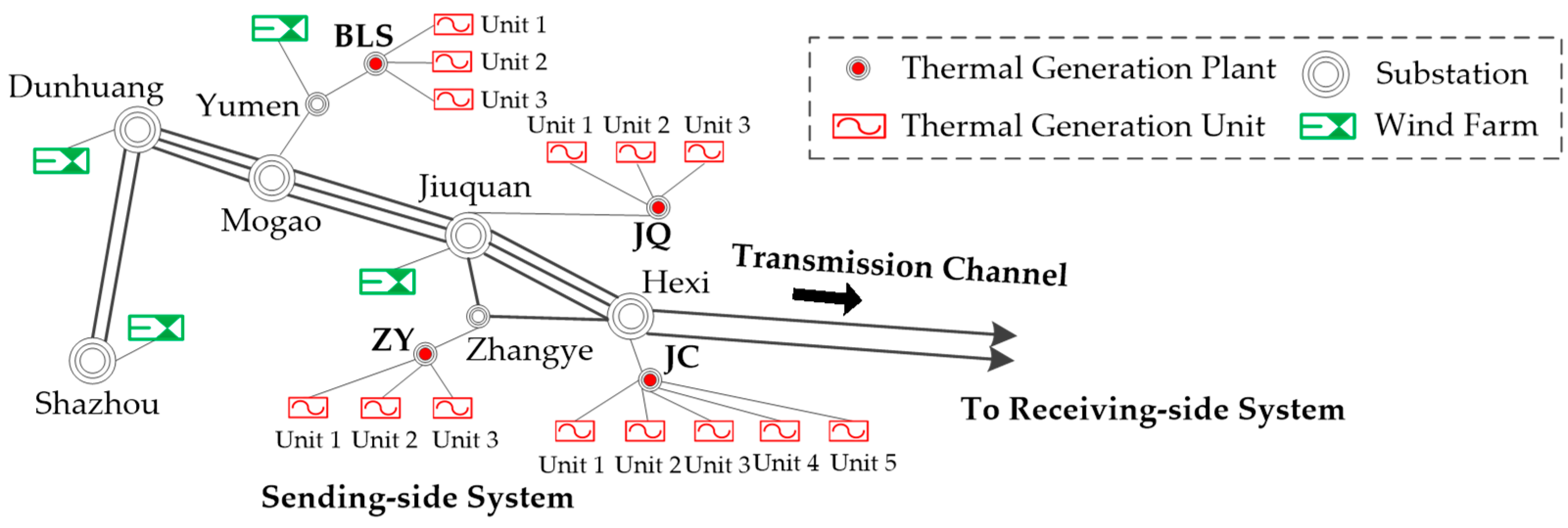
The simplified diagram of the large-scale wind power base sending-side system in Gansu Province is shown in Figure 8. The receiving-side system is equivalent to an infinity bus system. Hexi Substation is the border node in the sending-side that the transmission channel connects to. Four thermal generation plants are involved; the capacities of the units in each plant are shown in Table 1; and the relative parameters of each kind of unit are shown in Table 2. The electrical distance parameters that describe the grid topology are shown in Table 3 (the resistances of the lines are small and ignored). The base power is S B = 100   M V A in the system. While calculating the transient, stability-constrained TTC of the transmission channel, the transient models of the involved electronic components are used, and the relative parameters and the TTC calculation process are shown in the Appendix A.
The original day-head generation schedules are shown in Table 4. The four thermal generation plants are all online, and the thermal generation unit commitment and the generation schedule in each plant are based on the lowest generation cost rule. The corresponding original TTC is 4404 MW. Due to the restriction of TTC of the transmission channel, during period 1–10 (each period is one hour), the minimum allowable thermal generation is greater than the equivalent load, so the wind power is curtailed. The curtailed wind power is 5935 MWh.

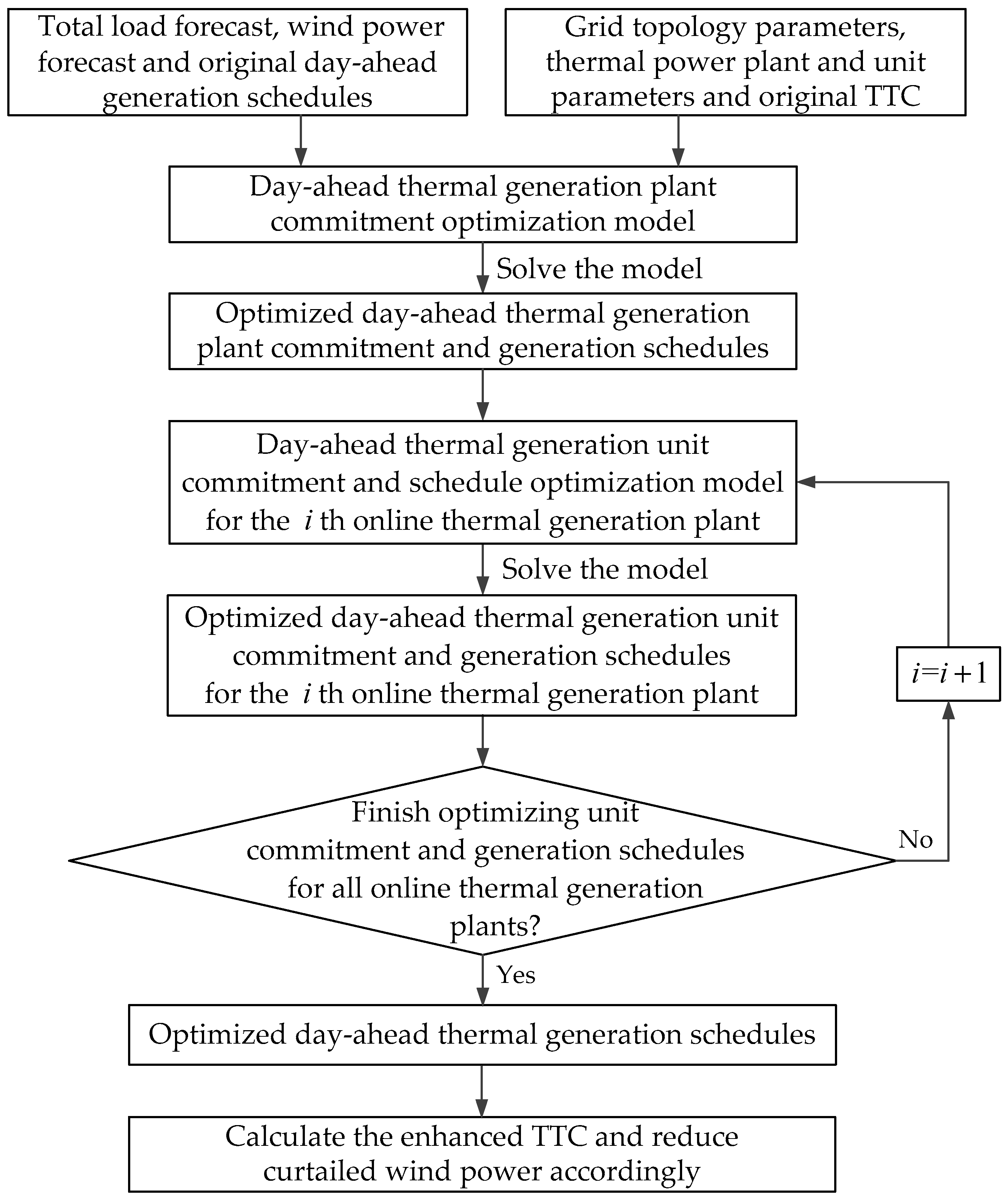
5.2. Analysis of the Results of Day-Ahead Thermal Generation Schedule Optimization

Establish the day-ahead thermal generation plant commitment optimization model and solve the model using the method in Section 4.2. The optimized day-ahead thermal generation plant commitment is obtained as shown in Table 5.
For the online thermal generation plants of JC, ZY and JQ, establish the day-ahead thermal generation unit commitment, schedule optimization models and solve the models using the method in Section 4.3, respectively. The optimized day-ahead thermal generation unit commitment and generation schedules are shown in Table 6 and Table 7.
The comparisons of the relative electrical parameters and generation costs of the sending-side system and the corresponding TTC before and after optimizing the day-head generation schedules are shown in Table 8. The detailed process of how to get the results in Table 8 is provided in the supplementary materials.
As shown in Table 8, by optimizing the day-ahead thermal generation schedules, the equivalent electrical distance between the transmission channel and the equivalent synchronous generator of the sending-side system decreases by 0.0483 p.u. and the equivalent inertia constant of the sending-side system increases by 7.57 s. The corresponding TTC is enhanced from 4404 to 5105 MW. The explanation of the TTC enhancement is as follows: Compared to the original day-head thermal generation schedules, the optimized generation schedules choose the thermal generation plants which are electrically closer to the transmission channel to be online, and shut down the BLS thermal generation plant which is the farthest plant from the transmission channel; therefore, the equivalent electrical distance between the transmission channel and the equivalent synchronous generator of the sending-side system is decreased; what is more, the optimized day-ahead thermal generation unit commitment inside each online plant chooses the thermal generation units with bigger inertia constants to be online; therefore, the equivalent inertia constant of the sending-side system is increased. Due to the decreased equivalent electrical distance, the electrical connection between the sending-side system and the transmission channel becomes tighter, and due to the increased equivalent inertia constant, the rotor angle accelerates slowly after a fault occurs, and this improves the transient stability of the system. Therefore, while the power delivered through the transmission channel is still 4404 MW, the system has not reached the transient stability critical state, and the power delivered through the transmission channel can increase to 5105 MW, which is the TTC after the day-head generation schedules are optimized.
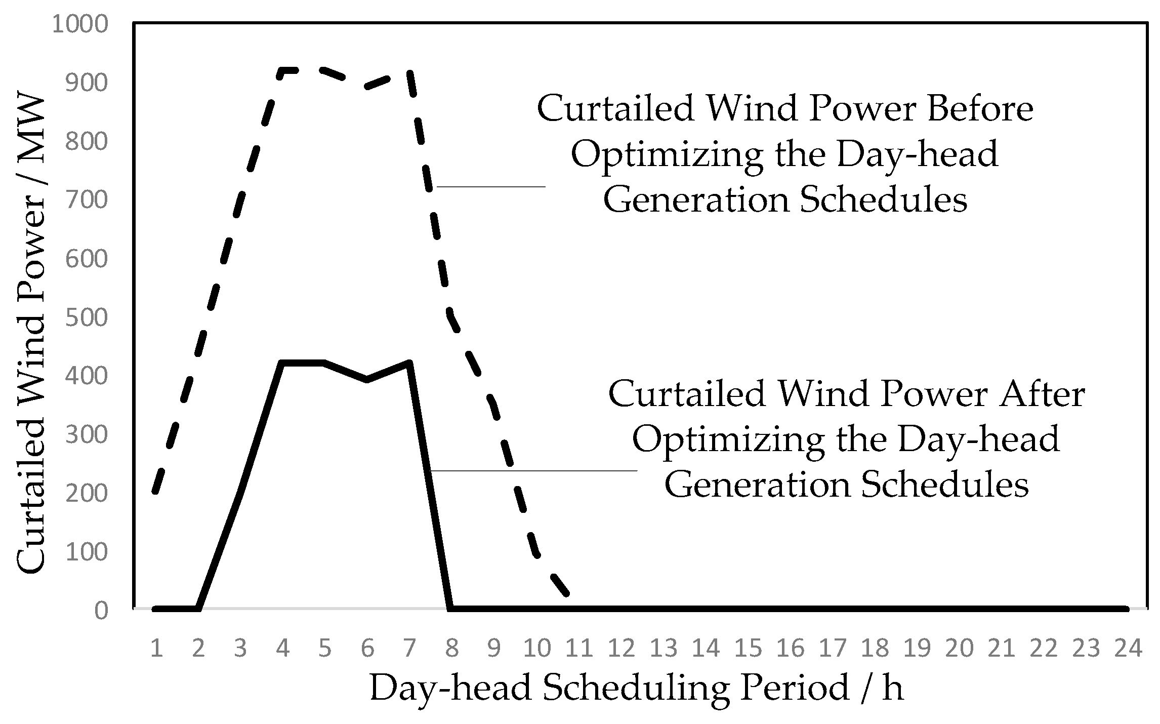
Using the enhanced TTC, the curtailed wind power can be reduced. The comparation of curtailed wind power before and after optimizing the day-head generation schedules is shown in Figure 9.
As shown in Figure 9, the curtailed wind power is reduced by 4083 MWh, and the benefit from it is $274,214 assuming the tariff of wind power is 67.16 $/MWh. As shown in Table 8, the thermal generation cost increases by $186,013. In general, the economic benefit brought by optimizing the day-ahead thermal generation schedules to enhance TTC is $88,201. It can be seen that, for the purpose of enhancing TTC, some of the units which are electrically closer to the transmission channel and with bigger inertia are constant while those with higher generation costs (like the Unit 4 and Unit 5 in JC thermal generation plant) are chosen to be online, and that increases the generation cost. However, the benefit from consuming the curtailed wind power because of the enhanced TTC is more than the additional generation cost, and the general cost is reduced. Therefore, the proposed method is economically favorable.

5.3. Suitable Parameter Selection for MOPSO

While solving the day-ahead thermal generation unit commitment and schedule optimization models in Section 4.3.1, we use the MOPSO in Section 4.3.2, and the initial population, generation of random members, termination criterion and other parameters in MOPSO have certain effects on the results. Taking the day-ahead thermal generation unit commitment and schedule optimization model solution of JC thermal generation plant as an example, the suitable parameters for solving the models are selected through comparation and sensitivity analysis as follows.
1. Initial population
There are three commonly used initial solutions in the day-ahead thermal generation unit commitment and schedule optimization problem, and they are used as initial populations in MOPSO respectively, as follows:
Initial population A: day-ahead generation schedules obtained based on the lowest generation cost rule.
Initial population B: day-ahead generation schedules obtained based on the installation capacity proportion rule.
Initial population C: random day-ahead generation schedules.
The objective results of JC thermal generation plant obtained from the above three initial populations are shown in Table 9. It can be seen in Table 9 that the equivalent inertia constant results are the same; this is because the day-ahead thermal generation unit commitments obtained from these three different initial populations are the same. Initial population A can get the lowest thermal generation cost because it is originally obtained based on the lowest generation cost rule. Therefore, we chose initial population A as the initial population in Section 5.2.
2. Generation of random members and inertia weight
In the velocity update equation (Equation (13)), the generation of random members r 1 , r 2 and the value of inertia weight ω effect the global search capability of MOPSO. 
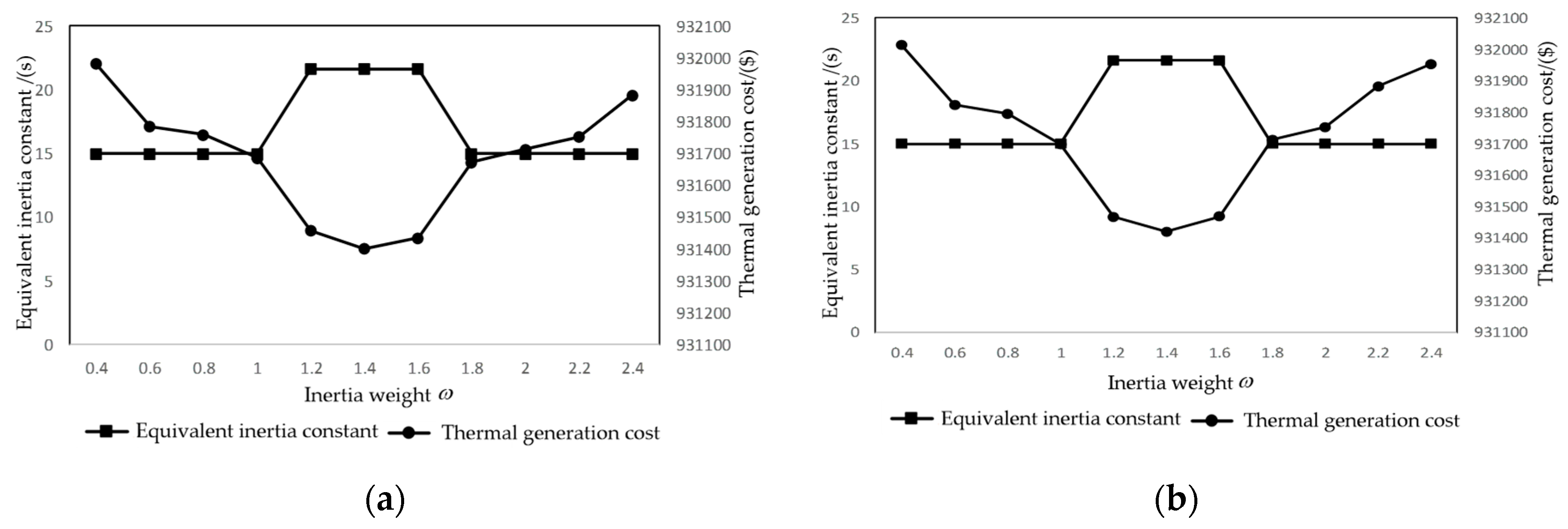
Figure 10 shows the objective results based on different generation methods of random members and different values of inertia weight. In Figure 10a,b, the random members are generated by uniform random sampling in [0,1] and Monte Carlo sampling in [0,1], respectively, and the inertia weights range from 0.4 to 2.4.
It can be seen from Figure 10 that the generation method of random members has little effect on the results. However, the value of inertia weight significantly influences the results, and when the value is near 1.4, MOPSO gets the best global search capability, and this is because if the value of inertia weight is too small, the results will fall into the local optimal solution, and if the value of inertia weight is too big, the results may miss the global optimal solution. Therefore, we used uniformly random sampling to generate random members for simplicity, and we let the inertia weight take the value of 1.4 in Section 5.2.
3. Termination criterion
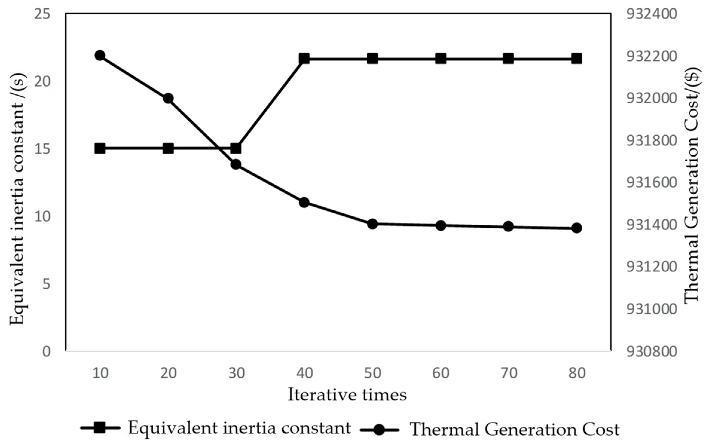
The termination criterion, which is the maximum number of iterations of MOPSO should consider when converging on the objectives. Figure 11 shows the convergence situation of the objectives as the number of iterations increases. It can be seen that when the number of iterations is more than 50, both equivalent inertia constant and thermal generation cost converge to their optimal values. Therefore, the maximum number of iterations is set to 55 as the termination criterion in Section 5.2.

6. Conclusions

Enhancing TTC allows more wind power to be delivered through the transmission channel to the load center, and it is of great importance to help consume wind power in the large-scale wind power base sending-side system. This paper proposed a new method to enhance TTC based on the existing grid structure; namely, by optimizing the day-ahead thermal generation schedules. It can significantly enhance TTC, and therefore, reduce the curtailed wind power. The conclusions are as follows:
  • TTC increases with the decrease of the equivalent electrical distance between the transmission channel and the equivalent synchronous generator of the sending-side system. TTC increases with the inertia constant of the equivalent synchronous generator of the sending-side system.
  • Optimizing the day-ahead thermal generation plant commitment with the objective of minimizing the equivalent electrical distance between the transmission channel and the equivalent synchronous generator of the sending-side system, and then optimizing the day-ahead thermal generation unit commitment and schedule considering the objective of maximizing the equivalent inertia constant can significantly enhance TTC, and therefore, help consume the curtailed wind power.
The proposed method in this paper enhances TTC by optimizing the day-ahead thermal generation schedules; thus, it achieves a reduction of curtailed wind power, and it is of great significance to help improve wind power consumption in the sending-side system with large-scale wind power integration.

Supplementary Materials

The following are available online at https://www.mdpi.com/1996-1073/13/9/2375/s1, PDF: Some Detailed Calculation Processes of the Results.

Author Contributions

Conceptualization, Y.Z.; methodology, Y.Z. and W.L.; validation, Y.Z. and Y.H.; investigation, Y.Z. and Y.H.; writing—original draft preparation, Y.Z.; writing—review and editing, W.L. and N.W.; supervision, W.L. and Q.Z. All authors have read and agreed to the published version of the manuscript.

Funding

This research was funded by National Key Technologies R&D Program (number 2015BAA01B04) and Project of State Grid Corporation of China (number SGGSKY00FJJS1800025).

Conflicts of Interest

The authors declare no conflict of interest.

Appendix A

The generators in the sending-side system are thermal generation units and wind power generators. The thermal generation units are simulated using synchronous generators, and their transient reactance is shown in Table A1. The wind farms are simulated using doubly-fed induction generators (DFIG). The active power control mode of the DFIG is maximum power point tracking and the reactive power control mode is constant power factor control. The transient relevant parameters are shown in Table A2.
Table A1. Transient parameters of units in each thermal generation plant.
Thermal Generation PlantUnit NumberTransient Reactance/(p.u.)
JCUnit 10.0256
Unit 20.0256
Unit 30.0256
Unit 40.0277
Unit 50.0282
ZYUnit 10.0282
Unit 20.0291
Unit 30.0291
JQUnit 10.0256
Unit 20.0277
Unit 30.0282
BLSUnit 10.0282
Unit 20.0291
Unit 30.0291
Table A2. Transient relevant parameters of DFIG.
Transient ParametersValues
Stator resistance 0.00706 p.u.
Rotor resistance0.005 p.u.
Stator leakage inductance0.171 p.u.
Rotor leakage inductance0.156 p.u.
Magnetizing inductance2.9 p.u.
Taking the TTC calculation of the original day-head generation schedules as an example, the TTC calculation process is as follows:
  • Based on the original day-head generation schedules in Table 4, take the generation schedule of period 1 as the initial operation point.
  • Increase the outputs of the wind farms in proportion to their original outputs, and decrease the outputs of the generators in the receiving-side system equally, and perform power flow calculations and a transient stability time domain simulation to check that the system is able to stay stable when an N-1 fault occurs on the transmission channel.
  • Repeat step 2, and the maximum steady state power that can be delivered through the transmission channel is 4404 MW, provided the system is able to stay transiently stable after a fault occurs. Therefore, the TTC of the original day-head generation schedules is 4404 MW.

References

  1. Zhu, D.; Liu, W.; Hu, Y.; Wang, W. A Practical Load-Source Coordinative Method for Further Reducing Curtailed Wind Power in China with Energy-Intensive Loads. Energies 2018, 11, 2925. [Google Scholar] [CrossRef] [Green Version]
  2. Liao, S.; Xu, J.; Sun, Y.; Bao, Y.; Tang, B. Control of Energy-Intensive Load for Power Smoothing in Wind Power Plants. IEEE Trans. Power Syst. 2018, 33, 6142–6154. [Google Scholar] [CrossRef]
  3. Ma, H.; Yan, Z.; Li, M.; Han, D.; Han, X.; Song, Y.; Wei, P.; Li, G.; Liu, Y. Benefit Evaluation of the Deep Peak-regulation Market in the Northeast China Grid. IEEE Comput. Appl. Power CSEE J. Power Energy Syst. 2019, 5, 533–544. [Google Scholar]
  4. Peng, F.; Gao, Z.; Hu, S.; Zhou, W.; Sun, H.; Wang, Z. Bilateral Coordinated Dispatch of Multiple Stakeholders in Deep Peak Regulation. IEEE Access 2020, 8, 33151–33162. [Google Scholar] [CrossRef]
  5. Yao, X.; Yi, B.; Yu, Y.; Fan, Y.; Zhu, L. Economic analysis of grid integration of variable solar and wind power with conventional power system. Appl. Energy 2020, 264, 114706. [Google Scholar] [CrossRef]
  6. Lu, M.S.; Chang, C.L.; Lee, W.J.; Wang, L. Combining the Wind Power Generation System with Energy Storage Equipment. IEEE Trans. Ind. Appl. 2009, 45, 2109–2115. [Google Scholar]
  7. Bitaraf, H.; Rahman, S. Reducing Curtailed Wind Energy Through Energy Storage and Demand Response. IEEE Trans. Sustain. Energy 2018, 9, 228–236. [Google Scholar] [CrossRef]
  8. Hou, L.; Li, W.; Zhou, K.; Jiang, Q. Integrating flexible demand response toward available transfer capability enhancement. Appl. Energy 2019, 251, 113370. [Google Scholar] [CrossRef]
  9. Fang, R.; Shang, R.; Wang, Y.; Guo, X. Identification of vulnerable lines in power grids with wind power integration based on a weighted entropy analysis method. Int. J. Hydrogen Energy 2017, 42, 20269–20276. [Google Scholar] [CrossRef]
  10. Hou, G.; Vittal, V. Determination of Transient Stability Constrained Interface Real Power Flow Limit Using Trajectory Sensitivity Approach. IEEE Trans. Power Syst. 2013, 28, 2156–2163. [Google Scholar] [CrossRef]
  11. Gholipour, E.; Saadate, S. Improving of Transient Stability of Power Systems Using UPFC. IEEE Trans. Power Deliv. 2005, 20, 1677–1682. [Google Scholar] [CrossRef]
  12. Johansson, N.; Ängquist, L.; Nee, H.P. An Adaptive Controller for Power System Stability Improvement and Power Flow Control by Means of a Thyristor Switched Series Capacitor (TSSC). IEEE Trans. Power Syst. 2010, 25, 381–391. [Google Scholar] [CrossRef]
  13. Paital, S.R.; Ray, P.K.; Mohanty, A. Comprehensive review on enhancement of stability in multimachine power system with conventional and distributed generations. IET Renew. Power Gener. 2018, 12, 1854–1863. [Google Scholar] [CrossRef]
  14. Varma, R.K.; Rahman, S.A.; Vanderheide, T. New Control of PV Solar Farm as STATCOM (PV-STATCOM) for Increasing Grid Power Transmission Limits During Night and Day. IEEE Trans. Power Deliv. 2015, 30, 755–763. [Google Scholar] [CrossRef]
  15. Yossef, D.; Tali, I.; Yehonatan, R.; Dror, M.; Danping, L.; Zeev, Z. Silicon-coated gold nanoparticles nanoscopy. J. Nanophotonics 2016, 10, 036015. [Google Scholar]
  16. Vegerhof, A.; Barnoy, E.A.; Motiei, M.; Malka, D.; Danan, Y.; Zalevsky, Z.; Popovtzer, R. Targeted Magnetic Nanoparticles for Mechanical Lysis of Tumor Cells by Low-Amplitude Alternating Magnetic Field. Mater. Spec. Issue Nanoprobes Imaging 2016, 9, 943. [Google Scholar] [CrossRef] [Green Version]
  17. Ariff, M.A.M.; Pal, B.C.; Singh, A.K. Estimating Dynamic Model Parameters for Adaptive Protection and Control in Power System. IEEE Trans. Power Syst. 2015, 30, 829–839. [Google Scholar] [CrossRef] [Green Version]
  18. Jiang, Y.; Yu, S.; Wen, B. Monthly electricity purchase and decomposition optimization considering wind power accommodation and day-ahead schedule. Int. J. Electr. Power Energy Syst. 2019, 107, 231–238. [Google Scholar] [CrossRef]
  19. Salkuti, S.R. Day-ahead thermal and renewable power generation scheduling considering uncertainty. Renew. Energy 2019, 131, 956–965. [Google Scholar] [CrossRef]
  20. Paudyal, S.; Ramakrishna, G.; Sachdev, M.S. Application of Equal Area Criterion Conditions in the Time Domain for Out-of-Step Protection. IEEE Trans. Power Deliv. 2010, 25, 600–609. [Google Scholar] [CrossRef]
  21. Romero, R.; Monticelli, A. A Zero-one Implicit Enumeration Method for Optimizing Investments in Transmission Expansion Planning. IEEE Trans. Power Syst. 1994, 9, 1385–1391. [Google Scholar] [CrossRef]
  22. Pham, M.; Zhang, D.; Koh, C.S. Multi-Guider and Cross-Searching Approach in Multi-Objective Particle Swarm Optimization for Electromagnetic Problems. IEEE Trans. Magn. 2012, 48, 539–542. [Google Scholar] [CrossRef]
  23. Ejebe, G.C.; Tong, J.; Waight, J.G.; Frame, J.G.; Wang, X.; Tinney, W.F. Available Transfer Capability Calculations. IEEE Trans. Power Syst. 1998, 13, 1521–1527. [Google Scholar] [CrossRef]
Figure 1. Schematic diagram of sending-side and receiving-side systems and a transmission channel.
Energies 13 02375 g001
Figure 2. Schematic diagram of the impact of enhancing total transfer capability (TTC) on reducing curtailed wind power.
Energies 13 02375 g002
Figure 3. (a) Diagram of a multi-generator sending-side system and receiving-side system and transmission channel; (b) diagram of an equivalent sending-side system and receiving-side system and transmission channel.
Energies 13 02375 g003
Figure 4. Diagram of power-angle curves when the system is in a transient stability critical state.
Energies 13 02375 g004
Figure 5. (a) Diagram of power-angle curves when X Σ = X Σ 0 . (b) Diagram of power-angle curves when X Σ = X Σ 1 .
Energies 13 02375 g005
Figure 6. (a) Diagram of power-angle curves when T J = T J 0 . (b) Diagram of power-angle curves when T J = T J 2 .
Energies 13 02375 g006
Figure 7. Flow diagram of the optimal day-ahead thermal generation scheduling method.
Energies 13 02375 g007
Figure 8. Simplified diagram of the large-scale wind power base sending-side system in Gansu Province.
Energies 13 02375 g008
Figure 9. Comparation of curtailed wind power before and after optimizing the day-head generation schedules.
Energies 13 02375 g009
Figure 10. (a) Objective results with random members generated by uniformly random sampling; (b) objective results with random members generated by Monte Carlo sampling.
Energies 13 02375 g010
Figure 11. Convergence situation of the objectives as the number of iterations increases.
Energies 13 02375 g011
Table 1. Capacities of units in each thermal generation plant.
Thermal Generation PlantUnit NumberUnit Capacity/
(MW)
JCUnit 1500
Unit 2500
Unit 3500
Unit 4300
Unit 5200
ZYUnit 1200
Unit 2100
Unit 3100
JQUnit 1500
Unit 2300
Unit 3200
BLSUnit 1200
Unit 2100
Unit 3100
Table 2. Parameters of each kind of thermal generation unit.
Unit Capacity/
(MW)
Inertia Constant/
(s/100 MW)
Generation Cost Parameters
a/($)b/($/MWh)c/($/(MW)2 h)
5001.50200380.040
3002.63230450.045
2003.12260460.051
1003.59300650.080
Table 3. Electrical distance parameters.
LinesReactance/(p.u.)LinesReactance/(p.u.)
Hexi-JC0.080Jiuquan-Mogao0.250
Hexi-Zhangye0.433Mogao-Shazhou0.071
Hexi-Jiuquan0.426Mogao-Yumen0.135
Zhangye-Jiuquan0.519Mogao-Dunhuang0.013
Zhangye-ZY0.530Yumen-BLS0.061
Jiuquan-JQ0.22
Table 4. Original day-head generation schedules and curtailed wind power/(MW).
Day-Head Scheduling PeriodJCZYJQBLSCurtailed Wind Power
Unit 1Unit 2Unit 1Unit 1Unit 1
1300300120300120201
2300300120300120436
3300300120300120700
4300300120300120920
5300300120300120920
6300300120300120892
7300300120300120920
8300300120300120500
9300300120300120350
1030030012030012096
113683681473681470
123663661463661460
133673671473671470
144114111644111640
153713711483711480
163743741493741490
173813811523811520
184474471794471790
194414411774411770
204004001604001600
214134131654131650
223793791523791520
233963961583961580
244094091644091640
Table 5. Optimized day-ahead thermal generation plant commitment.
Thermal Generation PlantOn/Off StateEquivalent Reactance/(p.u.)
JC10.1074
ZY1
JQ1
BLS0
Table 6. Optimized day-ahead thermal generation unit commitment.
Thermal Generation PlantUnit NumberOn/Off StateEquivalent Inertia Constant
/(s)
JCUnit 1121.63
Unit 20
Unit 30
Unit 41
Unit 51
ZYUnit 107.18
Unit 21
Unit 31
JQUnit 1113.74
Unit 20
Unit 31
Table 7. Optimized day-ahead thermal generation schedules/(MW).
Day-Head Scheduling PeriodJCZYJQ
Unit 1Unit 4Unit 5Unit 2Unit 3Unit 1Unit 3
13001801206060300120
23001801206060300120
33001801206060300120
43001801206060300120
53001801206060300120
63001801206060300120
73001801206060300120
83001801206060300120
93001801206060300120
103001801206060300120
113682211477474368147
123662191467373366146
133672201477373367147
144112471648282411164
153712231487474371148
163742241497575374149
173812281527676381152
184472681798989447179
194412651778888441177
204002401608080400160
214132481658383413165
223792281527676379152
233962381587979396158
244092451648282409164
Table 8. Comparation of relative electrical parameters, generation cost and TTC before and after optimizing the day-head generation schedules.
Equivalent Reactance/(p.u.)Equivalent Inertia Constant/(s)Thermal Generation Cost/($)TTC/(MW)
Before0.107434.981,732,5784404
After0.059142.551,918,5915105
Table 9. Comparation of objective results of JC thermal generation plant based on the above three initial populations.
Initial Population AInitial Population BInitial Population C
Equivalent Inertia Constant/(s)21.6321.6321.63
Thermal Generation Cost/($)931,402931,671932,085

