The Impact of SMOS Soil Moisture Data Assimilation within the Operational Global Flood Awareness System (GloFAS)

Abstract

In this study the impacts of Soil Moisture and Ocean Salinity (SMOS) soil moisture data assimilation upon the streamflow prediction of the operational Global Flood Awareness System (GloFAS) were investigated. Two GloFAS experiments were performed, one which used hydro-meteorological forcings produced with the assimilation of the SMOS data, the other using forcings which excluded the assimilation of the SMOS data. Both sets of experiment results were verified against streamflow observations in the United States and Australia. Skill scores were computed for each experiment against the observation datasets, the differences in the skill scores were used to identify where GloFAS skill may be affected by the assimilation of SMOS soil moisture data. In addition, a global assessment was made of the impact upon the 5th and 95th GloFAS flow percentiles to see how SMOS data assimilation affected low and high flows respectively. Results against in-situ observations found that GloFAS skill score was only affected by a small amount. At a global scale, the results showed a large impact on high flows in areas such as the Hudson Bay, central United States, the Sahel and Australia. There was no clear spatial trend to these differences as opposing signs occurred within close proximity to each other. Investigating the differences between the simulations at individual gauging stations showed that they often only occurred during a single flood event; for the remainder of the simulation period the experiments were almost identical. This suggests that SMOS data assimilation may affect the generation of surface runoff during high flow events, but may have less impact on baseflow generation during the remainder of the hydrograph. To further understand this, future work could assess the impact of SMOS data assimilation upon specific hydrological components such as surface and subsurface runoff.

1. Introduction

Hydrological predictability, amongst other factors, is linked with the initial hydrological conditions (IHC) within a catchment [1]. For example, ensemble streamflow prediction (ESP) methods used in seasonal streamflow forecasts depend on accurate estimates of the IHCs [2]. Of these IHCs, soil moisture is highly important, as the gradual release of water from the soil column is often a large component of streamflow. It has been shown that an accurate estimate of initial soil moisture enhances streamflow predictability at both short [3] and seasonal time scales [4]. This is because the hydrological prediction chain starts with the IHC’s which are used to initialise a hydrological model, then forcings from numerical weather prediction (NWP) forecasts are used to produce a streamflow forecast. Accurate measurements of initial soil moisture conditions are therefore beneficial to the operational global streamflow forecasts that have become available in recent years [5].

Operational streamflow forecasts can benefit from accurate initial soil moisture measurements by assimilating them into their IHC’s. Measurements can be obtained from in-situ observations from frequency domain reflectometry (FDR [6]) or cosmic ray methods such as the Cosmic-ray Soil Moisture Observing System (COSMOS [7,8]). However these measurements have low spatial representativeness [9] as they rely on point measurements and they do not have global coverage. Alternatively, measurements from satellite-based remote sensing platforms can provide global coverage. These can either come from active or passive microwave sensors, the former can have a high spatial resolution (~1 km for Synthetic Aperture Radar (SAR) sensors) but low repeat pass coverage (>10 days) [9]. Passive microwave sensors conversely have coarse spatial resolution but high repeat pass coverage, this second attribute makes them highly suitable for use within operational streamflow forecast systems.

Passive microwave sensors onboard satellite platforms such as Soil Moisture Active Passive (SMAP [10]), Soil Moisture and Ocean Salinity (SMOS [11]) and the Advanced Microwave Scanning Radiometer-2 (AMSR-2 [12]) can provide global soil moisture estimates [13]. The sensors detect brightness temperature from the top 1–5 cm of the soil column, which can then be transformed into an estimate of the soil moisture through methods including radiative transfer [14] and neural networks [15,16]. The broad swath width (~1000 km) combined with the short repeat pass times (~1–2 days) allow for frequent updating of the soil moisture status, which is beneficial for operational forecasting [17].

Remotely sensed soil moisture observations are typically incorporated into the IHC’s of a streamflow prediction system through data assimilation [9], using the ensemble Kalman filter for example [18,19]. Some previous studies have shown that this results in improved streamflow prediction [20], whilst others have seen a deterioration [21]. These results may relate to how challenges such as uncertainties and biases within the satellite data are dealt with [9,22].

Many of these previous studies however have performed their evaluations of soil moisture data assimilation using level 2 or 3 quality data. This additional post-processing of the original level 1 data, whilst improving the quality, also increases the latency time, meaning that it cannot be integrated within a real time operational forecast system. Instead either the original level 1 data or emulated level 2 data via a neural network, for example [15,16], can be assimilated within an operational forecast system. One example is the Integrated Forecast System (IFS) of the European Centre for Medium Range Weather Forecasts (ECMWF), whose land data assimilation system (LDAS) assimilates this soil moisture information from ASCAT (Advanced Scatterometer) and SMOS [23,24,25,26] into the soil moisture analysis.

The ECMWF operational soil moisture analysis, amongst other land surface analysis variables, is then used within the configuration of the Global Flood Awareness System (GloFAS [27,28]) to produce streamflow forecasts. In this configuration, the land surface analysis variables are used within the Hydrology Tiled ECMWF Scheme for Surface Exchanges of Land (H-TESSEL) land surface model component of the IFS [29] to produce forecasts of hydrological variables including surface and subsurface runoff. These are then coupled offline with the kinematic channel routing of the LISFLOOD hydrological model [30] to produce streamflow forecasts.

Since the GloFAS configuration is initialised from the IFS land surface analysis, it is likely that the assimilation of data including soil moisture has an impact upon streamflow prediction. Previous work has demonstrated a discernable impact of data assimilation upon GloFAS streamflow prediction, especially in areas dominated by snowmelt [31]. However the specific impact of the soil moisture data assimilation has not been assessed. The inclusion of SMOS within the IFS LDAS, as part of model cycle 46r1 in June 2019 [23], provides an opportunity to assess its impact upon GloFAS streamflow predictions.

The aim of this manuscript therefore is to describe our assessment of the impact of soil moisture data assimilation, from SMOS, upon streamflow prediction within GloFAS. This was be achieved by performing a data denial experiment using SMOS data and the GloFAS forecast configuration. Results from the experiment were analysed against in-situ streamflow observations to assess the impact upon GloFAS streamflow prediction skill. Then, an assessment against proxy streamflow observations from the GloFAS ERA-5 dataset [28] was performed to assess the global impact upon skill. Finally, the impact upon high and low flow prediction was assessed through direct comparison between the two GloFAS data denial experiments.

2. Materials and Methods

2.1. SMOS Soil Moisture Data

The SMOS satellite was launched in November 2009 with the aim of measuring soil moisture and ocean salinity. Onboard is an L-band radiometer which measures brightness temperature at 1400–1427 MHz [32,33]. At this frequency, the signal measured is sensitive to the soil moisture within the top few centimeters of the soil layer [34]. The level 1c data are provided at an average 43 km spatial resolution on the icosahedral equal area (ISEA)-4H9 grid, with a repeat cycle of less than 3 days [34]. The near real time level 1 brightness temperature is used for operational monitoring [24], as well as for research data assimilation experiments [35]. The level 2 soil moisture product is calculated from the level 1c data using a Bayesian approach which models the earth’s emissions at different polarisations and incidence angles to account for the interaction with vegetation [34]. Level 2 soil moisture accuracies ranged from 0.02–0.06 m³/m³ depending on the area and the radio frequency interference (RFI) [34]. However this level 2 is not available within the <3 h near real time (NRT) requirements of operational forecast systems, meaning it cannot be assimilated. In response a neural network (NN) processor has been developed using the level 1c data trained on the level 2 soil moisture data and the soil temperature from the ECMWF IFS [16]. A comparison of the level 2 and the level 1 NN products showed a standard deviation of the difference of 0.05 m³/m³ and a Pearson’s correlation coefficient higher than 0.7 in most regions of the globe [16]. It is important to note, however, that this study used SMOS soil moisture data created by a similar NN processor but trained on the ECMWF IFS soil moisture analysis, rather than the original level 2 product. This was to remove any bias between the SMOS soil moisture estimate and the IFS soil moisture analysis. The bias removal means the SMOS soil moisture data could be assimilated into the ECMWF IFS soil moisture analysis. ECMWF receives the SMOS level 1c data from ESA (European Space Agency) where it has already been converted from local solar time to UTC (Coordinated Universal Time), this enables it to be incorporated into the LDAS, which is based on UTC.

2.2. GloFAS Streamflow Predictions

As part of the European Commission Copernicus Emergency Management Service (CEMS) for floods, ECMWF operates the Global Flood Awareness System (GloFAS). This provides operational forecasts of streamflow once a day (00 UTC) at 0.1° spatial resolution globally with daily temporal resolution up to 46 days ahead. It was pre-operational since 2011 and has been operational since 23rd April 2018.

Streamflow forecasts are produced by coupling the hydrological forecasts of surface and subsurface runoff from the IFS H-TESSEL land surface model component [29] with the kinematic channel routing procedure within the LISFLOOD hydrological model [30]. The offline coupling is necessary because no lateral routing of runoff exists within H-TESSEL.

2.2.1. H-TESSEL Surface and Subsurface Runoff Forecasts

Surface and subsurface runoff were calculated from the H-TESSEL land surface model [29,36], which is part of the ECMWF IFS. The soil water budget in H-TESSEL was computed at each computational node using the Richards equation of water flow through the unsaturated soil profile [37]. At the top boundary layer water enters the soil as precipitation minus evaporation and runoff, at the bottom boundary layer water exits as free draining. The soil hydraulic conductivity was calculated from the van Genuchten equation which is a function of pressure head which in turn relates to the soil texture [38]. Different parameters are assigned to each soil texture class derived from the Food and Agriculture Organization dataset [39]. The saturated hydraulic conductivity was used to calculate the maximum infiltration rate which was then used to calculate the amount of runoff. Runoff is generated in a Hortonian manner when the throughfall plus the snowmelt exceeds the maximum infiltration rate [36].

The H-TESSEL forecasts were initialised from the ECMWF analysis fields. The analysis was produced by assimilating the first guess (i.e., the previous forecast) with the latest near real time hydro-meteorological observations. The LDAS of the IFS includes an analysis of soil moisture, which combines a two-dimensional screen level analysis of 2 metre temperature and relative humidity observations from SYNOP (Surface Synoptic Observations) with soil moisture observations from satellite sensors. A Simplified Extended Kalman Filter (SEKF) was used to analyse the soil moisture state vector for each grid point at each time step [17]. A more detailed description of the soil moisture data assimilation procedure can be found in the IFS documentation [36]. Currently satellite soil moisture observations from ASCAT and SMOS (the latter since model cycle 46r1 released 12th June 2019) are used within the LDAS soil moisture procedure. Therefore the assimilation of the SMOS soil moisture data into the ECMWF analysis may impact the GloFAS streamflow predictions.

2.2.2. LISFLOOD Channel Routing

The next stage of the GloFAS configuration is the offline coupling of the H-TESSEL surface and subsurface runoff forecasts with the kinematic channel routing from the LISFLOOD hydrological model. It routes the forecasted surface runoff from H-TESSEL along a one-dimensional channel network using a kinematic solution of the St. Venant equations [30]. Calculating this requires information about the channel length, gradient, flow width and depth, as well as the Manning’s roughness coefficient. This information was obtained firstly from the global river network database [40], which includes a river channel network at 0.1° spatial resolution from the digital elevation model (DEM) created by the Hydrological data and maps based on Shuttle Elevation Derivatives at multiple Scales project (HydroSHEDS project [41]). This is a hydrologically conditioned version of the original Shuttle Radar Topography Mission (SRTM) DEM [42] to ensure continuous stream networks. River widths are obtained from the Global Width Database for Large River (GWD-LR [43]). Bankfull water depth was estimated using the Manning’s equation applied to long term average discharge observations.

GloFAS also includes 463 large lakes and 667 reservoirs, whose locations and attributes were obtained from global datasets [44]. The outflow from each lake was computed using the relationship with lake level using the weir equation [45]. The extraction of water through irrigation is represented by subtracting from the forecasted streamflow a value taken from a monthly climatology [46]. Finally, open water evaporation is estimated using the Penman–Monteith with forcings taken from forecasts produced by the ECMWF IFS.

Eight of the GloFAS model parameters were tuned in a recent calibration exercise, including the channel Manning’s n, the multiplier for lake outflow and flood storage and outflow for reservoirs [46]. An evolutionary algorithm (EA) was used with the Kling–Gupta Efficiency metric (KGE [47]) calculated for streamflow as the objective function. The calibration was performed in 1287 catchments ranging from 484 km² to 4,800,000 km² in size. At each station, at least four years of observed daily streamflow data between 1995–2015 were required; these were mostly sourced from the Global Runoff Data Centre (GRDC [48]). The four-year observation sample was split into two years for calibration and two for validation. Within the former the calibration was performed using a maximum of 15 generations of the EA algorithm. Forcings of surface and subsurface runoff were obtained from the ECMWF IFS H-TESSEL reforecasts between 1995–2015 which were a combination of model cycles 41r1 and 41r2. Results from the calibration found improved streamflow estimation skill in 67% of the 1287 catchments (77% when excluding North America) [46]. The skill improvement was lowest where there were large negative biases in the baseline simulations, which could be caused by precipitation underestimation [46]. For catchments which were not part of the calibration exercise, default parameter values taken from the literature were used.

2.3. Streamflow Observations

In-situ observations of streamflow were extracted in order to perform a skill assessment of the GloFAS hydrological predictions. Observations were taken within the United States and Australia, as they have relatively dense observation networks and because previous studies have shown good performance of the SMOS soil moisture data. A total of 283 locations were chosen in the United States and 32 within Australia. These locations had been selected in a previous verification study of GloFAS [28] because they represented a range of different catchments found across the countries, as well as the catchments being sufficiently large to be captured by the comparatively coarse 0.1° × 0.1° spatial resolution of GloFAS. It was necessary to shift the latitude and longitude coordinate of each in-situ location on to the nearest GloFAS river cell. This is because the 0.1° × 0.1° GloFAS channel network is a simplification of the real-world channel locations, which can result in a small shift between the two. The shifting was done at each in-situ location by identifying the nearest channel cell in the GloFAS river network with a similar upstream area as the observed value. Additionally, a note was made at each in-situ site about the extent of any anthropogenic intervention in the hydrological functioning of the river, for example if there were any dams or irrigation activity.

In-situ streamflow observations were extracted from the respective monitoring agencies, as data for the time period of the GloFAS experiments was not already held. In Australia, the data were extracted from the Bureau of Meteorology (BoM). These were daily average streamflow observations which had been quality controlled. In the United States the data were extracted from the United States Geological Survey (USGS) and were six hourly average discharges. These were further averaged onto daily time steps, the units were converted from cubic feet per second to cubic metres per second. The observed time series at each in-situ location was assessed for missing data, and locations with less than 90% completeness were eliminated from the subsequent analysis.

2.4. GloFAS Experiment Design

To test the impact of SMOS data assimilation upon GloFAS streamflow prediction a data denial experiment using and excluding SMOS data was designed. Firstly, two ECMWF IFS analysis simulations were performed, one simulation included SMOS soil moisture data, described in Section 2.1, within the LDAS procedure, and the other simulation excluded it. The simulations were run at 06 and 18 UTC (Coordinated Universal Time) on each day from the 1st March 2017 to the 21st May 2018 using IFS cycle 45r1 upgraded to use IFS cycle 46r1 LDAS with grid TCo399 (Triangular Cubic-octahedral, approximately 0.25° × 0.25° horizontal resolution), climate version 015 and a 12 h assimilation window. This configuration of the LDAS was also used to support the operational implementation of the SMOS NN product assimilation in ECMWF IFS cycle 46r1 in June 2019 [23]. At 06 and 18 UTC on each day during the simulation period, the soil moisture analysis was created alongside the other LDAS products. These were used to initialise the ECMWF IFS to produce forecasts at a 6 hourly temporal resolution out to 24 h lead time. The outputs from these forecasts included the H-TESSEL forecasts of surface and subsurface runoff required for the LISFLOOD channel routing component of GloFAS.

The next stage of the experiment was to take the outputs from the two ECMWF IFS simulations and couple them with the channel routing component of GloFAS. The following output variables from the ECMWF IFS experiments were used as forcings within the channel routing: surface runoff, subsurface runoff, surface net solar radiation, surface net thermal radiation, 10 metre wind U component, 10 metre wind V component, 2 metre temperature, and 2 metre dewpoint temperature. The channel routing was performed at 24 h timesteps valid between 00–24 UTC, therefore the ECMWF IFS values needed to be aggregated onto each 24 h timestep. For accumulated variables, such as surface and subsurface runoff, the 24 h accumulations were aggregated by combining data from the following forecast times (

Table 1. 24 h accumulated variables created on a given day (d₀) were created by summarising the European Centre for Medium Range Weather Forecasts (ECMWF) Integrated Forecast System (IFS) experiment data at the forecast times shown below.

Forecast Time	Lead Time (hours)
d−1 at 18 UTC	6–12
d0 at 06 UTC	0–12
d0 at 18 UTC	0–6

):

For instantaneous variables, such as 2 metre temperature and the wind components, the average was taken across the instantaneous values at 00, 06, 12 and 18 UTC on the relevant day. All the ECMWF IFS forcings were re-gridded using nearest neighbour from the TCo399 grid onto the regular 0.1° × 0.1° grid (European Petroleum Survey Group—EPSG projection code 4326) used by GloFAS.

The aggregated and re-gridded ECMWF IFS forcings were then coupled with the LISFLOOD kinematic channel routing to produce daily streamflows for each day of the experiment period (1 March 2017–21 May 2018). for each 0.1° × 0.1° computational model cell. This GloFAS configuration of aggregating ECMWF IFS analysis forcings and coupling them to the LISFLOOD channel routing is the same as that used in the evaluation of GloFAS forced with ERA-5 data [28]. A summary of the datasets used in this experiment design are given in

Table 2. Summary of the datasets used in the Global Flood Awareness System (GloFAS) experiment. SMOS: Soil Moisture and Ocean Salinity; USGS: United States Geological Survey; H-TESSEL: Hydrology Tiled ECMWF Scheme for Surface Exchanges of Land; BoM: Bureau of Meteorology.

Dataset	Spatial Resolution (Degrees)	Temporal Resolution (Hours)
SMOS level 2 Soil Moisture (trained on ECMWF neural network)	0.50°	Instantaneous
H-TESSEL surface and subsurface runoff	0.25°	6
GloFAS Streamflow	0.10°	24
USGS streamflow observations	NA (point observations)	24
BoM streamflow observations	NA (point observations)	24

.

2.5. Streamflow Evaluation

2.5.1. Verification against In-Situ Observations

Results from the GloFAS streamflow experiments above were verified against in-situ observed streamflow values within Australia and the United States. Verification of both experiments was done to analyse the impact of SMOS data assimilation upon GloFAS prediction skill. The estimated streamflow from the two GloFAS experiments were extracted at each in-situ location on each day during the experiment period. Each GloFAS experiment was compared against the respective observations by calculating the modified Kling–Gupta Efficiency (KGE_mod) index [47,49]. The KGE_mod was calculated as a combination of the correlation, the bias and the variability (Equation (1)):

$$\begin{gathered} {\mathrm{KGE}}_{\mathrm{mod}}=1-\sqrt{{\left(r-1\right)}^2+{\left(\beta -1\right)}^2+{\left(\gamma -1\right)}^2} \\ r=\frac{co{v}_{s,o}}{{\sigma }_s·{\sigma }_0}, \beta =\frac{{\mu }_s}{{\mu }_o}, \gamma =\frac{{\sigma }_s/{\mu }_s}{{\sigma }_o/{\mu }_o} \end{gathered}$$

(1)

where r = correlation, β = bias, γ = variability, s = simulation (i.e., the GloFAS experiment), o = observation, cov = covariance, σ = standard deviation and μ = mean.

The KGE_mod is very useful for diagnosing the performance of a hydrological simulation, as it combines three of the most important factors in producing good results. However great care must be taken if interpreting its results as a skill score owing to the lack of a benchmark predictor [50]. Therefore a skill score [51] was computed to compare the KGE_mod results from the GloFAS simulations with and without SMOS soil moisture data assimilation (KGE_modSS Equation (2)). Positive values showed where the GloFAS simulation, which includes the assimilation of SMOS soil moisture data, outperforms the simulation without the assimilation of SMOS.

$${\mathrm{KGE}}_{\mathrm{mod}}\mathrm{SS}=\frac{{\mathrm{KGE}}_{\mathrm{mod}}\left[\mathrm{with}\mathrm{SMOS}\right]-{\mathrm{KGE}}_{\mathrm{mod}}\left(\mathrm{without}\mathrm{SMOS}\right)}{{\mathrm{KGE}}_{\mathrm{mod}}\mathrm{Perf}-{\mathrm{KGE}}_{\mathrm{mod}}\left(\mathrm{without}\mathrm{SMOS}\right)}$$

(2)

where KGE_modPerf = 1 which is a theoretical perfect score for the KGE_mod metric.

2.5.2. Global Impact upon GloFAS

The difficulty of obtaining global in-situ streamflow observations meant that it was not possible to assess the global impact of SMOS data assimilation through a skill score comparison. Instead the assessment was done by calculating the 5th and 95th streamflow percentiles in each GloFAS model cell over the whole experiment period for both experiments. These percentiles represent the low and high flow values respectively. The percentiles were calculated on the specific discharge values, which is the discharge divided by the upstream area, as this removed the influence of the upstream catchment area size. The percentage differences in the percentile values between the two GloFAS experiments were then calculated. This analysis was chosen to highlight whether SMOS assimilation affected mostly high or low flows; this may have important consequences for a flood forecasting system. Another advantage of this assessment method was that it could be performed globally as it did not depend on the presence of in-situ observations. This allowed a complete global analysis of the impacts of SMOS data assimilation upon GloFAS.

3. Results

3.1. Verification against Observed Streamflow

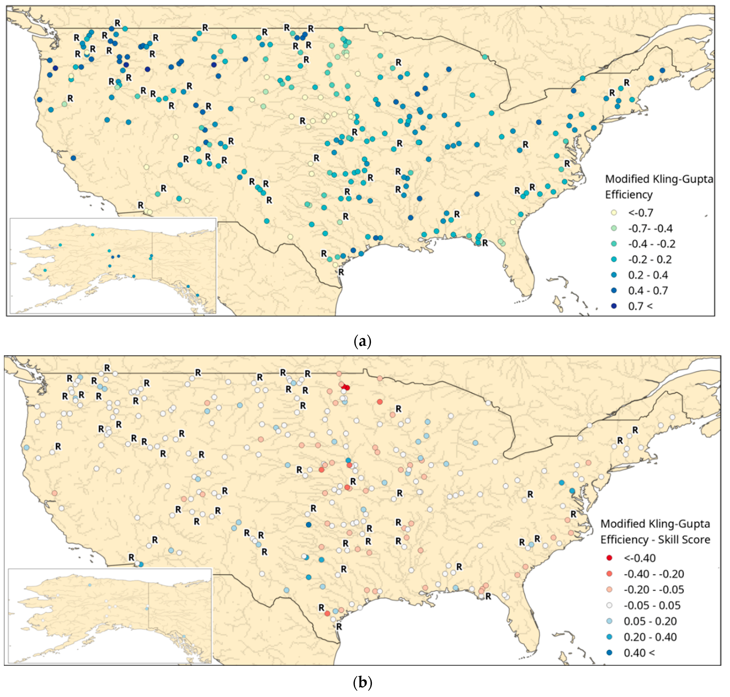
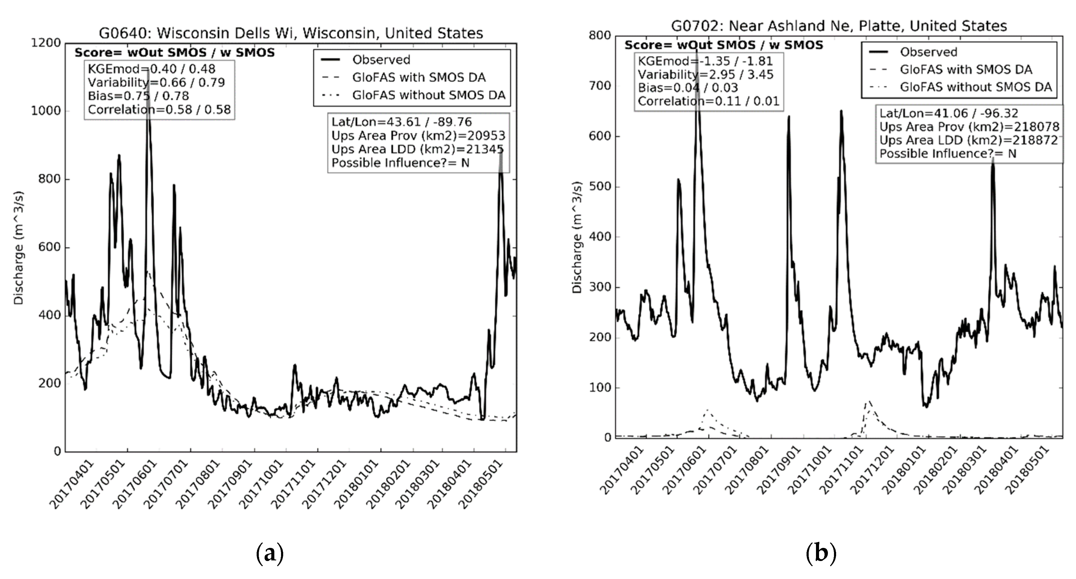
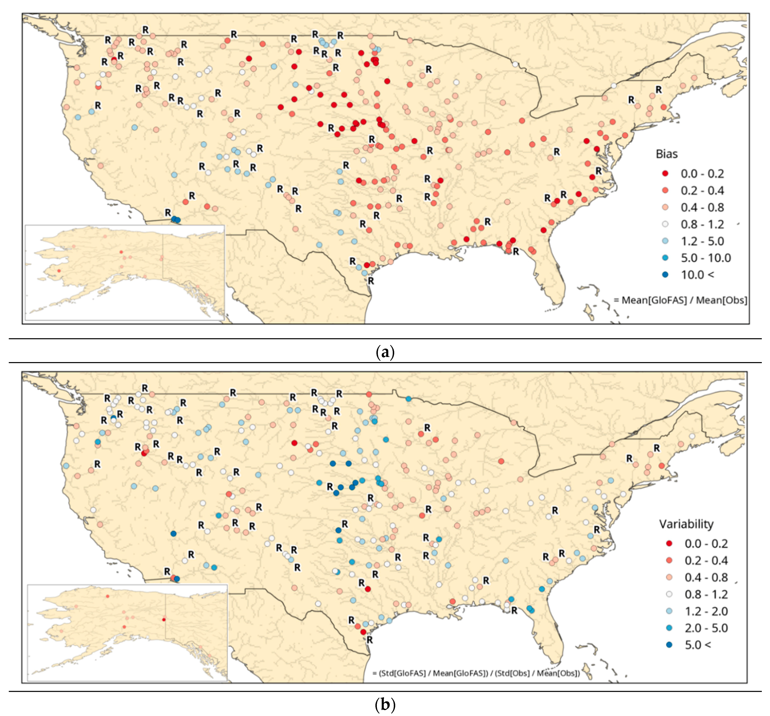
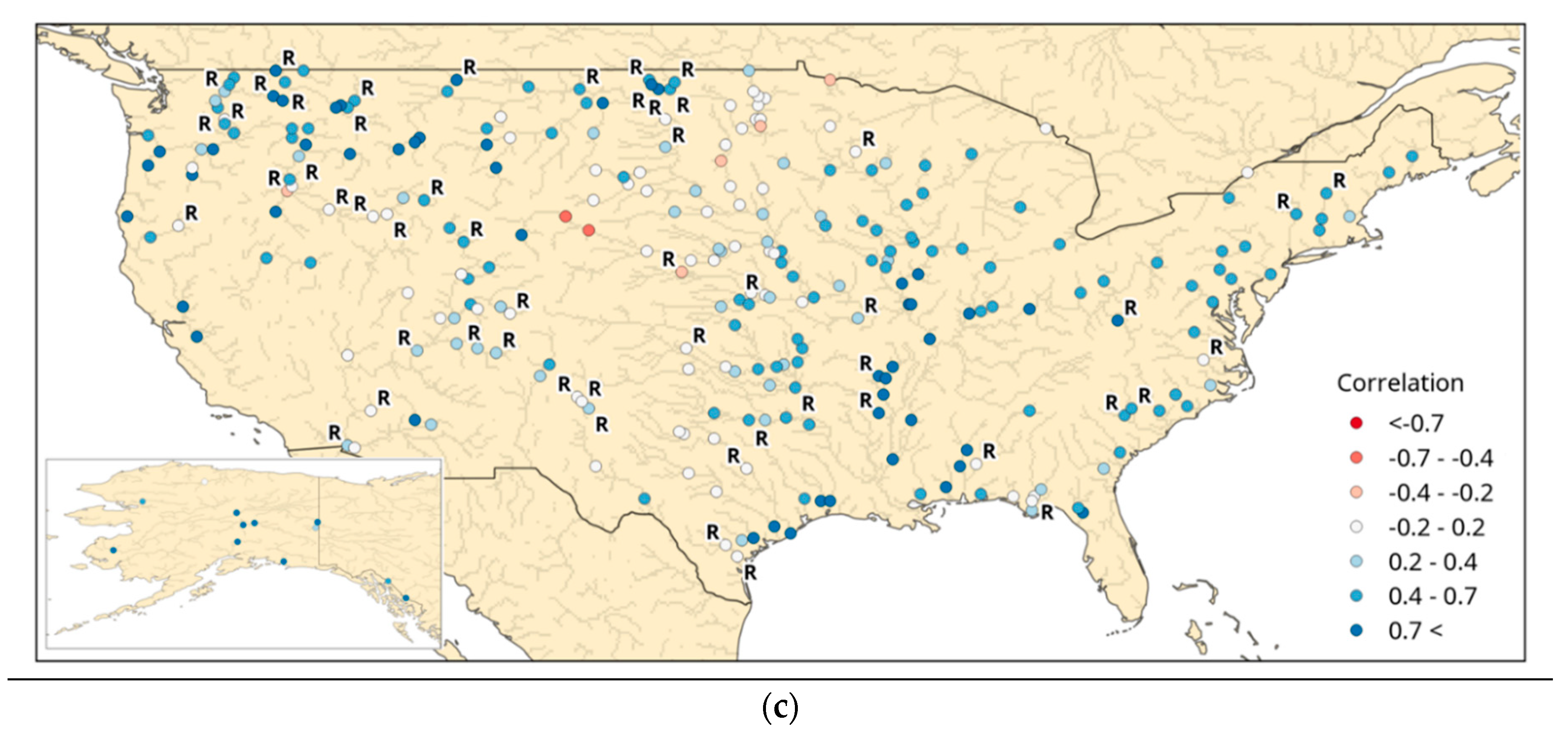
3.1.1. United States

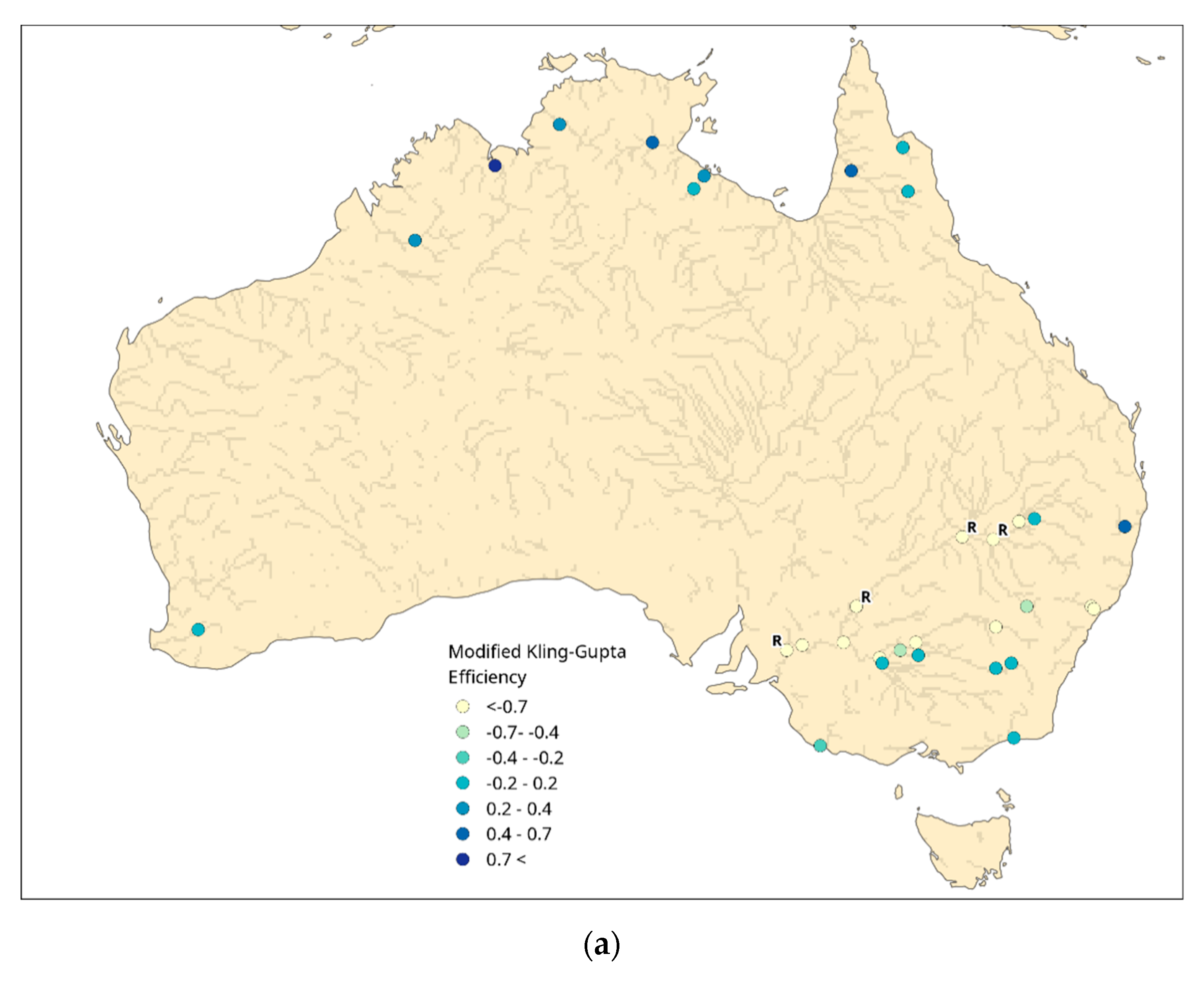
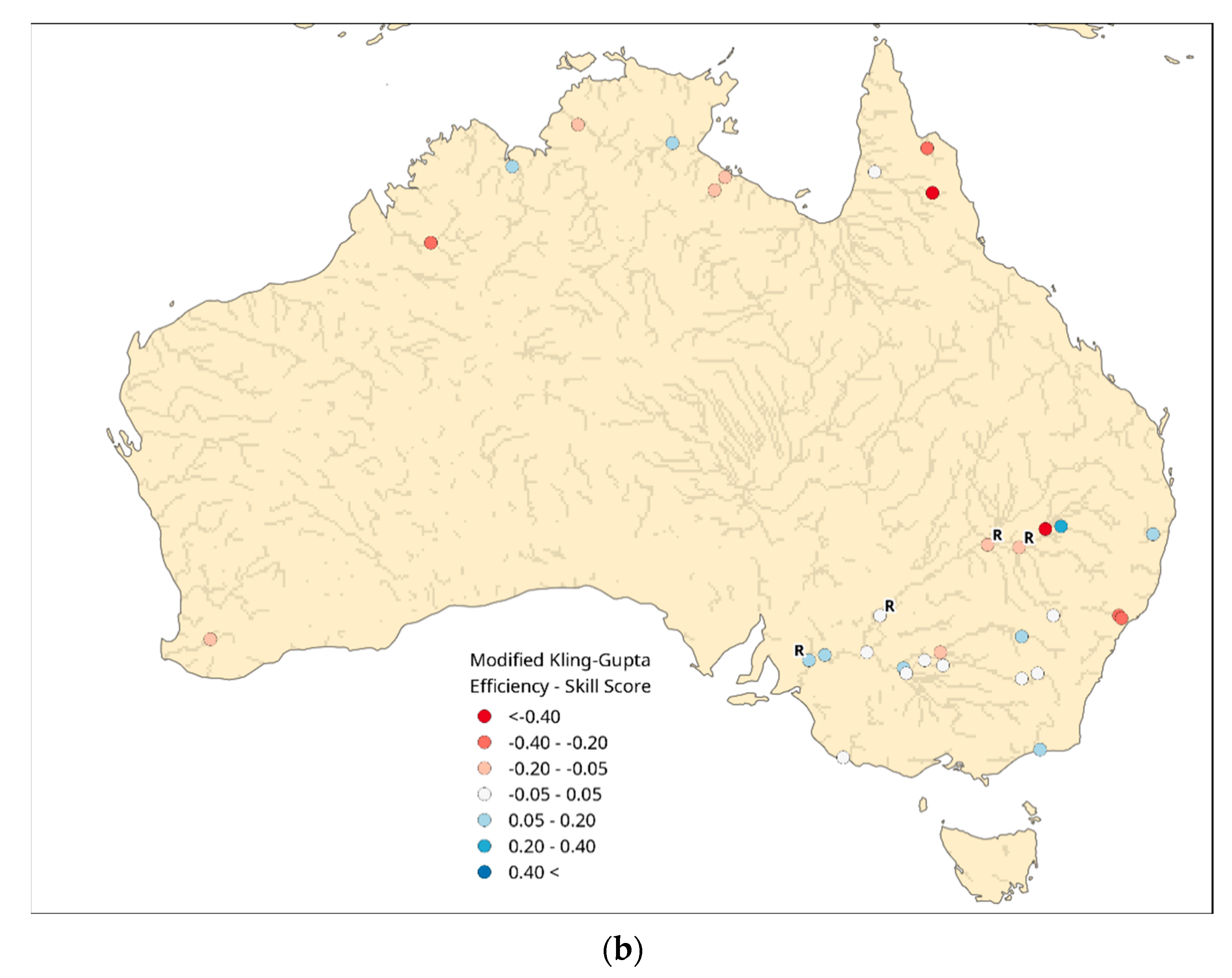
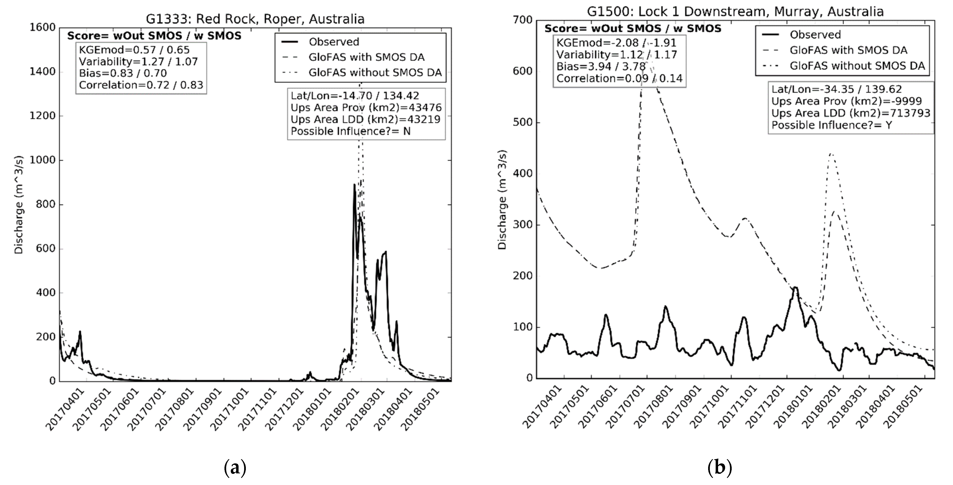
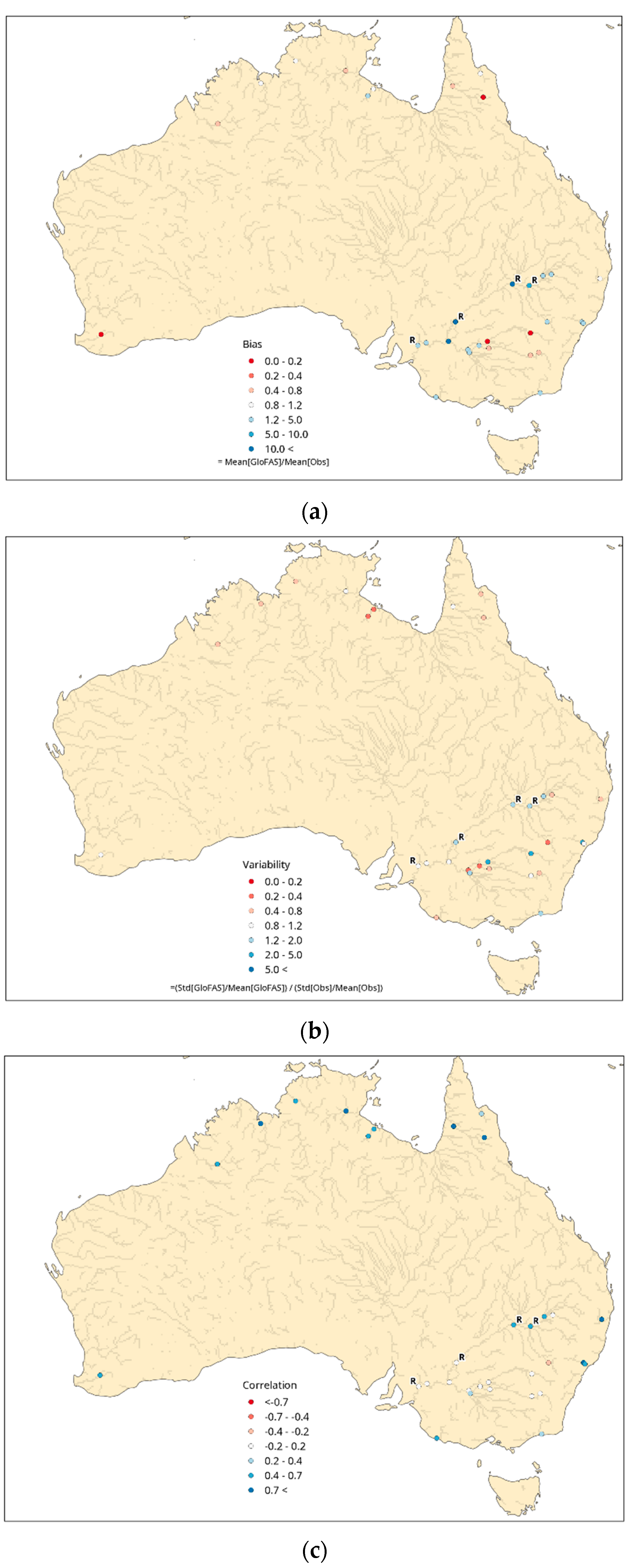
A wide range of KGE_mod scores occurred throughout the United States in the simulation with SMOS soil moisture data assimilation. A cluster of high values occurred in the north west in the Colombia and upper Missouri basins, a cluster of low scores occurred in the Platte River (Nebraska) (Figure 1a). One explanation for the wide range of scores could be the presence of regulation within the river basins, a process which was only simplistically represented by GloFAS at some locations. However there was no apparent correlation between the KGE_mod value and river regulation, as locations subject to regulation show both high and low KGE_mod values (Figure 1a).

The KGE_mod skill scores were mostly centred around 0 (Figure 1b), meaning that there was little difference between the skill of the simulations with and without SMOS soil moisture data assimilation. The largest negative KGE_mod skill score values appeared on the Platte River (Nebraska), as well as the upper Nelson River (North Dakota). At these locations the KGE_mod values were less than zero in both GloFAS simulations with and without SMOS data assimilation. Analysing the hydrograph near the outlet of the Platte River showed that both GloFAS simulated hydrographs were much below the observed discharge (Figure 2b). The main difference between them was the discharge peak which occurred on the 1 November 2017. This peak was greater in the simulation when SMOS soil moisture was assimilated, but because this coincides with a trough in the observations this may be what caused the lower skill owing to the poor correlation. Further analysis in the Platte River found that GloFAS simulates three reservoirs within this basin (at Kingsley, Seminoe and Pathfinder). These could explain the low KGE_mod values in this basin as they may over-estimate the total reservoir storage and/or under-estimate the total outflow from one of, or all of, the reservoirs.

There were 40 locations where the KGE_mod skill score was 0.05 or more (Figure 1b), 31 of these locations had low KGE_mod values (less than 0.40), meaning that care must be taken when interpreting the apparent improvements at these locations. Two locations within the Wisconsin River demonstrated positive KGE_mod skill scores and KGE_mod values greater than 0.40. At one of these locations, both GloFAS simulations captured the overall rise and fall within the observed discharge series, but neither captured the observed variability (Figure 2a). The GloFAS simulation which included the assimilation of SMOS soil moisture had a large streamflow peak in May 2017 which better matched the observations, hence increasing the KGE_mod. However the peak was still not as sharply defined as in the observations (Figure 2a).

Across all 283 gauging station locations in the United States the GloFAS simulation with SMOS soil moisture data assimilation shows slightly improved bias and KGE_mod values over the simulation without SMOS soil moisture data assimilation (

Table 3. Streamflow evaluation metrics averaged across the 283 United States gauging stations.

Simulation	R	Bias	KGEmod
Without SMOS DA	0.428	0.840	−0.504
With SMOS DA	0.420	0.812	−0.472

). A previous study [52] also investigated the hydrological impact of SMOS data assimilation, but within the upper Mississippi basin. Whilst that study did not explicitly analyse streamflow, they found that CDF matching of modelled soil moisture from the Variable Infiltration Capacity (VIC) model to SMOS soil moisture resulted in higher values [53]. This could explain the higher KGE_mod values observed at some locations in the GloFAS experiment which had SMOS soil moisture data assimilation. For example at the Wisconsin river (Figure 2) the higher streamflow in June 2017 in the GloFAS experiment with SMOS could be the result of higher soil moisture values leading to more generation of surface runoff.

The KGE_mod from the simulation with SMOS data assimilation was broken down into its constituent components of bias, variability and correlation (Figure 3). This was done to explain the trends in the KGE_mod score above (Figure 1). For the bias, values less than 1 showed that GloFAS under-estimates streamflow with the reverse being true for values greater than 1. In this assessment, GloFAS mostly had an under-estimation bias with some over-estimation in the south west (Figure 3a). The greatest under-estimation occurred within the Platte River, which, as discussed above, could be related to the treatment of reservoir storage within GloFAS (Figure 2). The variability showed that GloFAS has a higher variability than the observations in locations where the KGE_mod score was low (Figure 3b). At the Platte River, the GloFAS variability being higher than the observations occurred due to its baseflow making it more sensitive to the peak flows which occurred in June and November 2017 (Figure 2). At the same location, the GloFAS simulation with SMOS soil moisture data assimilation had a higher variability than the simulation without SMOS, due to the greater November 2017 peak flow in the former simulation (Figure 2). Correlation was greater than zero in most locations across the US, with 164 locations having a correlation greater than 0.4 (Figure 3c). Locations with the highest correlation also had higher KGE_mod scores. There was little difference in the correlation scores at these locations between the GloFAS simulations with and without SMOS soil moisture data assimilation (Figure 2).

3.1.2. Australia

The KGE_mod values from the GloFAS simulation which included SMOS soil moisture data assimilation show that values greater than 0.2 occur in the north of Australia (Figure 4). For example, in the Roper River both GloFAS simulations captured the peak streamflows between January and April 2018 (Figure 5). Both GloFAS simulations miss the observed peak in April 2017, but both capture the extremely low baseflow from May 2017 to January 2018, which may be the main cause of the higher KGE_mod value at this location. The GloFAS simulation which included SMOS soil moisture data assimilation had a lower peak flow in February 2018 than the GloFAS simulation without SMOS (Figure 5). This better matched the observed peak flow at this time and may explain why the KGE_mod value rose from 0.57 to 0.65 when SMOS soil moisture data assimilation was included (Figure 5).

KGE_mod values in the south east of Australia were mostly less than zero (Figure 4a). The majority of these locations lie within the Murray–Darling river basin, which features a large amount of regulation to the natural river flow [53]. Large quantities of water are extracted from the Murray–Darling river for purposes including the irrigation of agricultural land, and consequently the observed streamflow would be lower than the original natural flow. The hydrographs near the outlet of the basin demonstrate this issue whereby both GloFAS simulations are greater than the observed streamflow (Figure 5). Additionally the shape of both simulated GloFAS hydrographs did not match that of the observations. GloFAS includes three reservoirs within this basin, but evidently these are insufficient to represent the full impact of the water management regime within the basin. At this location, the GloFAS simulation with SMOS soil moisture data assimilation has lower peak flows than the GloFAS simulation without SMOS, something that also occurred in the north of the country (Figure 5).

The KGE_mod skill score in Australia showed a decline in KGE_mod scores in the north of the country and in the upper Murray–Darling basin when SMOS soil moisture data were assimilated (Figure 4b). However, in 9 locations the KGE_mod skill score is greater than 0.05, which shows an improvement when SMOS data were assimilated. All but two of these locations occurred within the Murray–Darling basin. The KGE_mod skill score values were often attributable to a difference in one or two flood peaks during the simulation period between the simulations with and without SMOS data assimilation. For example, at the outlet of the Murray–Darling basin the positive KGE_mod skill score value was due to the simulated peak in February 2018 being lower in the simulation which included SMOS data assimilation, which better matched the observation (Figure 5). However, for the rest of the simulation period, the two simulations were almost identical. It was not clear what particular aspect of the SMOS soil moisture data assimilation might be causing these trends in the KGE_mod skill score. Care should be taken when interpreting the KGE_mod skill score trends in the Murray–Darling basin, however, since neither GloFAS simulation captured the management processes.

Averaging the streamflow evaluation metrics across all 32 gauging stations showed a slight decline from the simulation which includes SMOS soil moisture data assimilation (

Table 4. Streamflow evaluation metrics averaged across the 32 Australian gauging stations.

Simulation	R	Bias	KGEmod
Without SMOS DA	0.410	2.466	−1.248
With SMOS DA	0.356	2.558	−1.340

). Previous studies have also investigated the impact of SMOS data assimilation upon streamflow prediction in the Murray–Darling basin using the VIC hydrological model [54,55]. Their results found that SMOS data assimilation slightly improved the streamflow evaluation metrics, in contrast to the results found here. The differences between this study and those of previous studies [54,55] could be because this study looks across all of Australia, rather than just at the Murray–Darling basin. Also, within the Murray–Darling, this study includes gauging locations near the outlet, whereas previous studies [54,55] have focueds on smaller catchments within the upper reaches. These smaller catchments may be less prone to water management processes, which may be negatively affecting the streamflow metrics in this study.

The components of the KGE_mod show that the bias of the GloFAS simulation tends towards over-estimation, particularly within the Murray–Darling basin (Figure 6). This was highlighted in the hydrograph at the outlet of the basin (Figure 5b) and likely reflected the lack of GloFAS’ ability to replicate the water management practices throughout the basin. For variability, the GloFAS simulation under-estimated it in the north of the country and is slightly over-estimated in the Murray–Darling basin (Figure 6). This could be due to GloFAS not under-estimating the magnitude of the flood peaks in the north of the country which would result in a lower standard deviation. In the Murray–Darling this is because the river management practices, not represented in GloFAS, aim to reduce the variability of the streamflow. The correlation was highest in the north of the country where river flows are more natural than in the Murray–Darling basin, where the correlation was lower (Figure 6).

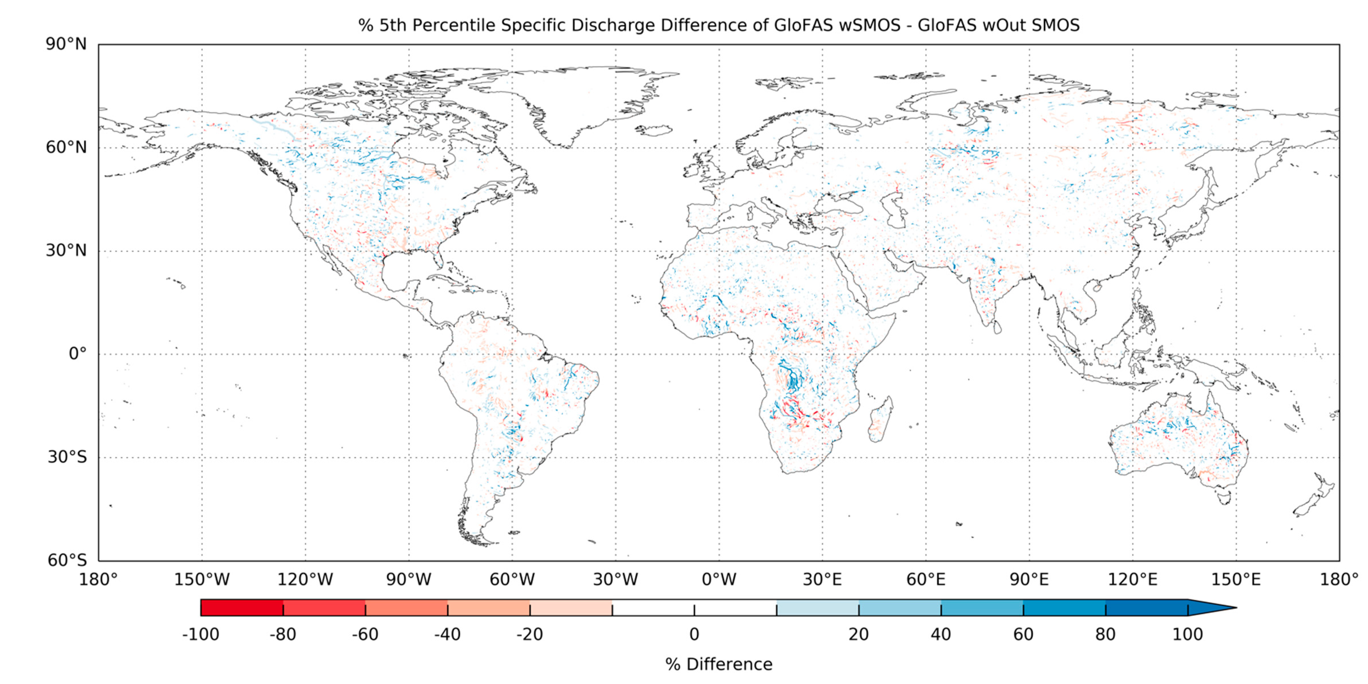
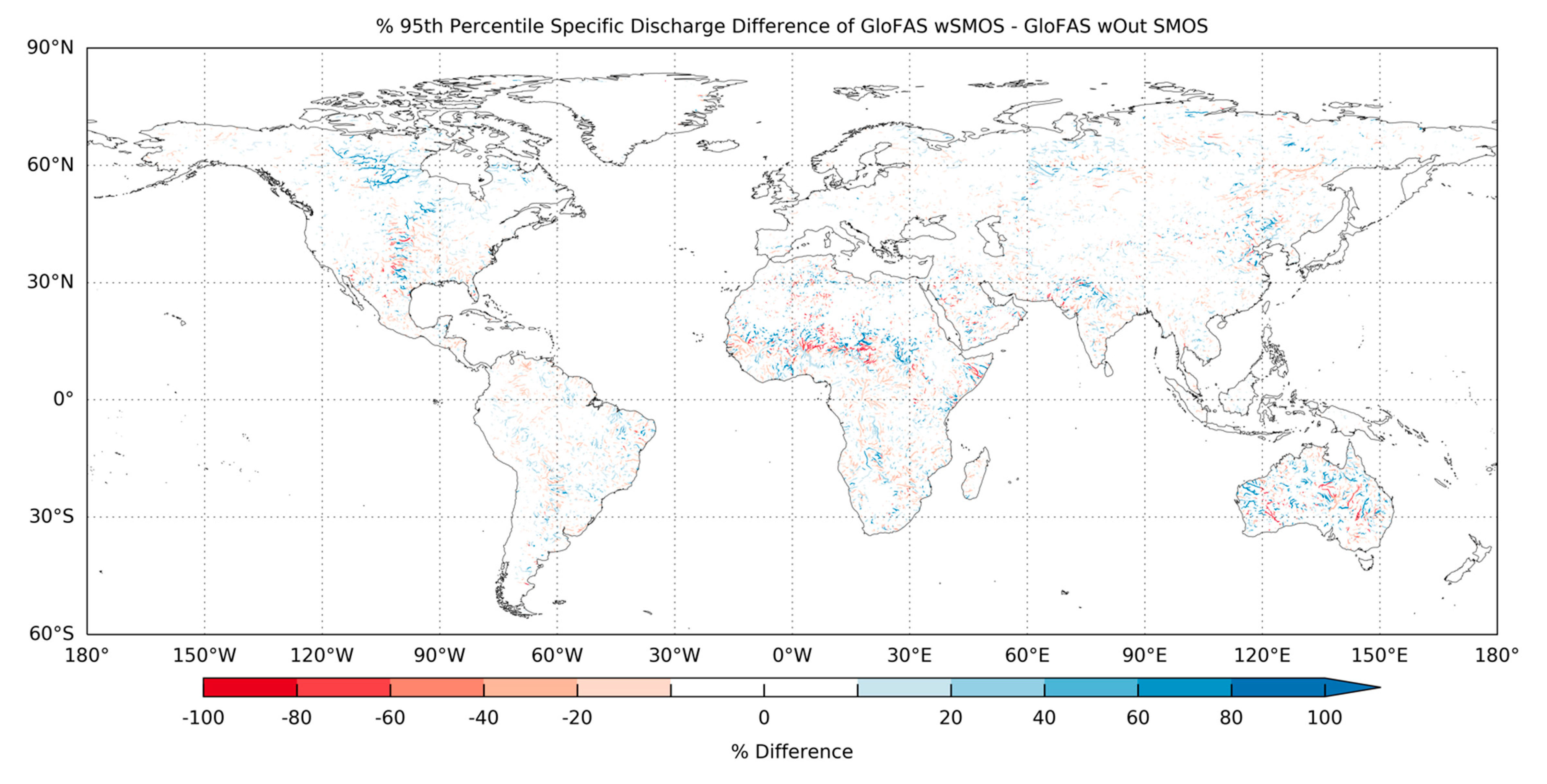
3.2. Global Impact upon GloFAS

Low flows in large parts of the world showed little impact from the assimilation of SMOS soil moisture data within GloFAS (Figure 7). The greatest percentage differences in low flows (the 5th flow percentile) were found around the Hudson Bay, southern Central Africa, Australia and the northern latitudes of Eurasia (Figure 7). At most of these locations, the 5th flow percentile had decreased after the assimilation of SMOS soil moisture data. There were only a few locations where the 5th flow percentile increases by a large amount, the strongest signal was in southern Africa at 15°S (Figure 7). However, care should be taken when interpreting percentage differences in the 5th flow percentile, as small differences in areas with very low flows can result in large percentage differences. For example, in southern Central Africa and Australia the 5th percentile flow values were in the order of ×10⁻⁴ mm·day⁻¹. However, this does not explain the strong signal around the Hudson Bay, as its 5th percentile values were greater than those of surrounding regions, which displayed minimal differences. Snow cover and snowmelt can play an important role in the hydrology of this region, however SMOS data should be masked during periods of snow cover, meaning that this explanation is unlikely. Instead, SMOS soil moisture data assimilation may have been increasing the soil H-TESSEL soil moisture during the summer period when low flows occurred. However, this would require further investigation.

High flows were also unaffected in large parts of the world, however the areas which were affected showed a stronger impact on high flows than for low flows (Figure 8). The areas with the greatest impact were the Hudson Bay, central United States, Australia, the Sahel region and to a lesser extent Pakistan/north west India and north eastern China. The Hudson Bay area showed a widespread increase in the 95th flow percentile after the assimilation of SMOS soil moisture into GloFAS (Figure 8). This could suggest that SMOS soil moisture assimilation was increasing the soil moisture in this region, which lead to an increase in both low and high flows. In the central United States the results agreed with the streamflow skill assessment in Section 3.1.1, which found that peak flows increased in rivers such as the Platte (Figure 2b), which decreased the KGE_mod skill score (Figure 1b). In the other regions, however, there was no clear spatial trend to these differences, as differences of opposing sign occurred close to each other. One example was in Australia, which showed increased high flows in the northern fringe of the country, but decreased flows in some areas of the Murray–Darling basin in the south east (Figure 8), which was also observed in Section 3.1.2 (Figure 5b).

4. Discussion

This study investigated the impact of SMOS soil moisture data assimilation upon GloFAS streamflow prediction within an operational forecast configuration. In general, only a minor impact on streamflow prediction skill was found. Globally, the greatest impact was found in the Hudson Bay, central United States, the Sahel and Australia. The greatest impact of SMOS was upon the simulation of flood peaks, lower flows showed lower sensitivity to the inclusion of SMOS data assimilation.

The areas of the world which showed the greatest impact upon high flows in this study appeared to coincide with areas which have open land cover (Figure 8). Comparing the results of this study against landcover data from the ESA Climate Change Initiative (CCI) dataset for 2018 [56] confirms that the greatest changes occurred in sparsely vegetated, herbaceous, grassland, cropland and shrubland classes. Forested and urban areas showed little impact of SMOS soil moisture data assimilation upon GloFAS streamflow predictions. This is likely because SMOS measurements in these areas are subject to interference, which increases the measurement error, meaning they were filtered out and are not assimilated into the model. It may be possible that certain land cover types are associated with either an improvement or a degradation of GloFAS streamflow skill with the assimilation of SMOS soil moisture data. To investigate this further, at each observation station location in the United States and Australia the land cover classification from the ESA CCI data for 2018 [56] were extracted. Then, all stations where the modified Kling–Gupta Efficiency skill score (KGE_modSS) was ≤−0.05 (indicating a degradation with SMOS data assimilation) and all the stations where KGE_modSS was ≥0.05 (indicating an improvement with SMOS data assimilation) were identified. Within each of the degradation and improvement categories, these were further broken down into the landcover classes from ESA CCI. Results showed that for both degradation and improvement most stations belonged to the grass, tree, water and shrub landcover classes (

Table 5. Modified Kling–Gupta efficiency skill score (KGE_modSS) values at station locations in the United States and Australia calculated from the GloFAS experiments with and without SMOS data assimilation broken down by ESA Climate Change Initiative (CCI) landcover class. The second column shows stations where KGE_modSS degraded with SMOS data assimilation, the third column shows where it improved.

ESA CCI Land Cover Type	Number of Stations where KGEmodSS ≤ −0.05 (%)	Number of Stations where KGEmodSS ≥ 0.05 (%)
Grass	16 (24%)	28 (21%)
Tree	13 (20%)	19 (14%)
Urban	7 (11%)	12 (9%)
Crop	4 (6%)	3 (2%)
Vegetation	0 (0%)	8 (6%)
Herbaceous	2 (3%)	11 (8%)
Water	11 (17%)	24 (18%)
Shrub	13 (20%)	29 (22%)

). Therefore it appears that the landcover status does not explain the spatial pattern of degradations or improvements in the GloFAS prediction skill.

SMOS data assimilation also appeared to have a minimal impact upon GloFAS results within Europe (Figure 7 and Figure 8). This could be because many of the rivers within Europe are below the 0.1° spatial resolution of GloFAS. Another reason could be the presence of radio frequency interference (RFI) in this region upon the SMOS measurements. This would mean that SMOS data are filtered out in this region and are not assimilated into the model.

The results suggest that the assimilation of SMOS soil moisture mostly affected high flows (Figure 8). Analysis of hydrographs in the United States and Australia confirmed that the main, and sometimes only, differences occurred in the peak flows during the experiment period (Figure 2 and Figure 5). It would be expected that altering the soil moisture may also affect the amount of water released to the river during low flows, however this was not observed in this study. The explanation could be that SMOS data assimilation mainly affects the top soil layer, and since this is only a very shallow portion of the entire soil column, this could explain the minimal impact on low flows. A greater impact on low flows could result if the soil moisture assimilation is then analysed into root zone soil moisture [20]. The ECMWF IFS LDAS already performs this root zone analysis with SMOS data, but perhaps greater weight should be given to the SMOS data; future work could investigate this. However since the assimilation mostly affects the top soil layer this could have a large impact on the ability of the soil column to generate surface runoff, as surface runoff is mostly produced in the top soil layer. For example, if SMOS data assimilation increases the soil moisture in the top soil layer, this reduces the infiltration capacity of this soil layer, meaning more surface runoff production during the next rainfall event and greater flow in the river.

The finding that SMOS data assimilation has a minor impact on GloFAS streamflow prediction corresponds with previous findings [22,57,58]. Previous studies have posited that the reasons for this include, amongst others, the representativeness of the soil layers, biases between the model and satellite data, the use of a calibrated hydrological model and uncertainties within the hydrological model [22,59]. Regarding the first of these the SMOS soil moisture data were assimilated into the top soil layer of the H-TESSEL soil column, which was 7 cm deep. This is comparable with the depth penetrated by the SMOS soil moisture measurements, which are in the order of a few centimeters [34].

Biases between the SMOS and H-TESSEL model soil moisture data were addressed by using the SMOS soil moisture neural network product trained on ECMWF IFS (i.e., H-TESSEL) soil moisture analysis. This would implicitly remove any biases between the SMOS observations and the ECMWF model. However this would restrict the data assimilation to only correcting for random model errors rather than also correcting the bias, preventing it from changing the behaviour of the soil moisture [55]. Assimilating the SMOS neural network product trained on the original SMOS level 2 soil moisture data could offer a solution, as this product is not bias corrected to the ECMWF model. However it would not currently work within the ECMWF IFS LDAS, as it breaks the assumption of the zero observation-model bias. A possible solution for future work would be to perform a parameter analysis of H-TESSEL, which may involve tuning the parameters which control the vertical soil water budget.

The use of a calibrated hydrological model to perform the streamflow predictions may explain the resulting minor impact of SMOS data assimilation. As mentioned above, GloFAS was calibrated in a previous study by optimizing the streamflow parameters using forcings from a 20 year ECMWF IFS reforecast [46]. The calibration of a given hydrological model can sometimes mean that it is difficult for any subsequent simulation to outperform it [58]. However the GloFAS calibration study only tuned the LISFLOOD streamflow parameters and left the vertical hydrological component, i.e., H-TESSEL soil water balance, unchanged. Hence, GloFAS is not as fully calibrated as other hydrological models, meaning there could be more scope for improving its streamflow prediction skill through data assimilation into its initial conditions. This is evidenced by the improvements observed at some locations in the United States whereby peak discharges better matched the observations after the assimilation of SMOS soil moisture (Figure 2). Increased soil moisture values from the assimilation of SMOS soil moisture could cause increased surface runoff production and hence greater streamflows [52].

Uncertainties within the GloFAS model configuration and parameterisation may also explain the minor impact of soil moisture data assimilation. They could represent biases and or errors which could not be overcome by data assimilation of soil moisture alone. In the United States, for example, GloFAS exhibits a widespread under-estimation bias (Figure 3a) whilst in Australia there was an over-estimation bias at most locations (Figure 6a). A possible solution for future work could be to revise the parameterisation of the H-TESSEL soil water budget using SMOS soil moisture data in a calibration procedure [22]. Biases within GloFAS could also be caused by the precipitation forcings, therefore, a dual updating procedure of both the precipitation and initial soil moisture conditions could be carried out in future work [60].

5. Conclusions

Overall, this study has analysed the impact of SMOS soil moisture data assimilation upon GloFAS streamflow predictions within an operational configuration. Two GloFAS experiments were conducted using hydro-meteorological forcings from ECMWF IFS experiments, which include and exclude the assimilation of SMOS soil moisture data. Streamflow predictions from both GloFAS experiments were evaluated against observations from in-situ measurements using the KGE_mod metric. The results showed some impact upon hydrological prediction skill, but it was difficult to discern a clear signal due to biases and uncertainties within GloFAS.

Further investigation was performed to determine how low and high flow GloFAS predictions were affected by SMOS data assimilation. Results showed that high flows were more affected than low flows. A global assessment of the impact upon low and high flows found the greatest impact around the Hudson Bay, central United States, the Sahel and Australia. However, there was no clear spatial trend to these results as differences of opposing sign were within close proximity to each other. Investigating the hydrographs at specific station locations found that differences in KGE_mod could often be attributed to differences in a single flood peak, whilst the remainder of the simulated hydrographs were very similar. In some instances the flood peak in the simulation with SMOS data assimilation was the greatest, whilst the opposite was true in other instances. This could be because SMOS data assimilation only affects the top soil layer, which can greatly alter the generation of surface runoff during a flood peak, but has little effect upon baseflow production during lower flows. There was no clear spatial trend to the changes in high and low flows either. To better understand these changes future work should focus on finding out how the SMOS data are affecting the GloFAS simulations. This could be done by analysing changes in individual hydrological components such as surface and subsurface runoff, the former being significant for high flows and the latter more important during low flows. This study highlights that assimilating SMOS soil moisture does impact the hydrological predictions of GloFAS, but more work is needed to understand the causes of the observed results.

References

1. Wood, A.W.; Lettenmeier, D.P. An ensemble approach for attribution of hydrologic prediction uncertainty. Geophys. Res. Lett. 2008, 34, 14401. [Google Scholar] [CrossRef] [Green Version]
2. Arnal, L.; Cloke, H.L.; Stephens, E.; Wetterhall, F.; Prudhomme, C.; Neumann, J.; Krzeminski, B.; Pappenberger, F. Skillful seasonal forecasts of streamflow over Europe? Hydrol. Earth Syst. Sci. 2018, 22, 2057–2072. [Google Scholar] [CrossRef] [Green Version]
3. Seo, D.; Lakhankar, T.; Cosgrove, B.; Khanbilvardi, R.; Zhan, X. Applying SMOS soil moisture data into the National Weather Service (NWS)’s Research Distributed Hydrologic Model (HL-RDHM) for flash flood guidance application. Remote Sens. Appl. Soc. Environ. 2017, 8, 182–192. [Google Scholar] [CrossRef]
4. Koster, R.D.; Mahanama, S.P.P.; Livneh, B.; Lettenmeier, D.P.; Reichle, R.H. Skill in streamflow forecasts derived from large-scale estimates of soil moisture and snow. Nat. Geosci. 2010, 3, 613–616. [Google Scholar] [CrossRef]
5. Emerton, R.E.; Stephens, E.M.; Pappenberger, F.; Pagano, T.C.; Weerts, A.H.; Wood, A.W.; Salamon, P.; Brown, J.D.; Hjerdt, N.; Donnelly, C.; et al. Continental and global scale flood forecasting systems. WIREs Water 2016, 3, 391–418. [Google Scholar] [CrossRef] [Green Version]
6. Robinson, D.A.; Campbell, C.S.; Hopmans, J.W.; Hornbuckle, B.K.; Jones, S.B.; Knight, R.; Ogden, F.; Selker, J.; Wendroth, O. Soil moisture measurement for ecological and hydrological watershed-scale observations: A review. Vadose Zone J. 2008, 7, 358–389. [Google Scholar] [CrossRef] [Green Version]
7. Zreda, M.; Shuttleworth, W.J.; Zeng, X.; Zweck, C.; Desilets, D.; Franz, T.; Rosolem, R. COSMOS: The COSmic-ray Soil Moisture Observing System. Hydrol. Earth Syst. Sci. 2012, 16, 4079–4099. [Google Scholar] [CrossRef] [Green Version]
8. Evans, J.G.; Ward, H.C.; Blake, J.R.; Hewitt, E.J.; Morrison, R.; Fry, M.; Ball, L.A.; Doughty, L.C.; Libre, J.W.; Hitt, O.E.; et al. Soil water content in southern England derived from a cosmic-ray soil moisture observing system COSMOS-UK. Hydrol. Process. 2016, 30, 4987–4999. [Google Scholar] [CrossRef] [Green Version]
9. Brocca, L.; Ciabatta, L.; Massari, C.; Camici, S.; Tarpanelli, A. Soil Moisture for Hydrological Applications: Open Questions and New Opportunities. Water 2017, 9, 140. [Google Scholar] [CrossRef]
10. Entekhabi, D.; Njoku, E.G.; O’Neill, P.E.; Kellogg, K.H.; Crow, W.T.; Edelstein, W.N.; Entin, J.K.; Goodman, S.D.; Jackson, T.J.; Johnson, J.; et al. The Soil Moisture Active Passive (SMAP) mission. Proc. IEEE 2010, 98, 704–716. [Google Scholar] [CrossRef]
11. Barre, H.J.M.P.; Duesmann, B.; Kerr, Y.H. SMOS: The mission and system. IEEE Trans. Geosci. Remote Sens. 2008, 46, 587–593. [Google Scholar] [CrossRef]
12. Kim, S.; Liu, Y.Y.; Johnson, F.M.; Parinussa, R.M.; Sharma, A. A global comparison of alternate AMSR2 soil moisture products: Why do they differ? Remote Sens. Environ. 2015, 161, 43–62. [Google Scholar] [CrossRef]
13. Ma, H.; Zeng, J.; Chen, N.; Zhang, X.; Cosh, M.H.; Wang, W. Satellite surface soil moisture from SMAP, SMOS, AMSR2 and ESA CCI: A comprehensive assessment using global ground based observations. Remote Sens. Environ. 2019, 231, 111215. [Google Scholar] [CrossRef]
14. Wigneron, J.-P.; Kerr, Y.; Waldteufel, P.; Saleh, K.; Escorihuela, M.-J.; Richaume, P.; Ferrazzoli, P.; de Rosnay, P.; Gurney, R.; Calvet, J.-C.; et al. L-band microwave emission of the biosphere (L-MEB) model: Description and calibration against experimental data sets over crop fields. Remote Sens. Environ. 2007, 107, 639–655. [Google Scholar] [CrossRef]
15. Rodríguez-Fernández, N.J.; Aires, F.; Richaume, P.; Kerr, Y.H.; Prigent, C.; Kolassa, J.; Cabot, F.; Jiménez, C.; Mahmoodi, A.; Drusch, M. Soil moisture retrieval using neural networks: Application to SMOS. IEEE Trans. Geosci. Remote Sens. 2015, 53, 5991–6007. [Google Scholar] [CrossRef]
16. Rodríguez-Fernández, N.J.; Muñoz Sabater, J.; Richaume, P.; de Rosnay, P.; Kerr, Y.H.; Albergel, C.; Drusch, M.; Mecklenburg, S. SMOS near-real-time soil moisture product: Processor overview and first validation results. Hydrol. Earth Syst. Sci. 2017, 21, 5201–5216. [Google Scholar] [CrossRef] [Green Version]
17. de Rosnay, P.; Drusch, M.; Vasiljevic, M.; Balsamo, G.; Albergel, C.; Isaksen, L. A simplified Extended Kalman Filter for the global operational soil moisture analysis at ECMWF. Q. J. R. Meteorol. Soc. 2013, 139, 1199–1213. [Google Scholar] [CrossRef]
18. López López, P.; Wanders, N.; Schellekens, J.; Renzullo, L.J.; Sutanudjaja, E.H.; Bierkens, M.F.P. Improved large-scale hydrological modelling through the assimilation of streamflow and downscaled satellite soil moisture observations. Hydrol. Earth Syst. Sci. 2016, 20, 3059–3076. [Google Scholar] [CrossRef] [Green Version]
19. Massari, C.; Camici, S.; Ciabatta, L.; Brocca, L. Exploiting satellite-based soil moisture for flood forecasting in the Mediterranean area: State update versus rainfall correction. Remote Sens. 2018, 10, 292. [Google Scholar] [CrossRef] [Green Version]
20. Brocca, L.; Moramarco, T.; Melone, F.; Wagner, W.; Hasenauer, S.; Hahn, S. Assimilation of surface- and root-zone ASCAT soil moisture products into rainfall-runoff modelling. IEEE Trans. Geosci. Remote Sens. 2012, 50, 2542–2555. [Google Scholar] [CrossRef]
21. Alvarez-Garreton, C.; Ryu, D.; Western, A.W.; Su, C.-H.; Crow, W.T.; Robertson, D.E.; Leahy, C. Improving operational flood ensemble prediction by the assimilation of satellite soil moisture: Comparison between lumped and semi-distributed schemes. Hydrol. Earth Syst. Sci. 2015, 19, 1659–1676. [Google Scholar] [CrossRef] [Green Version]
22. Li, Y.; Grimaldi, S.; Walker, J.P.; Pauwels, V.R.N. Application of remote sensing data to constrain operational rainfall-driven flood forecasting: A review. Remote Sens. 2016, 8, 456. [Google Scholar] [CrossRef] [Green Version]
23. ECMWF. ECMWF. ECMWF Part II: Data Assimilation. In IFS Documentation CY46R1 Operational Implementation 6 June 2019; ECMWF, Ed.; ECMWF: Reading, UK, 2019; p. 103. Available online: https://www.ecmwf.int/en/elibrary/19306-part-ii-data-assimilation (accessed on 30 March 2020).
24. de Rosnay, P.; Muñoz Sabater, J.; Albergel, C.; Isaksen, L.; English, S.; Drusch, M.; Wigneron, J.-P. SMOS brightness temperature forward modelling and long term monitoring at ECMWF. Remote Sens. Environ. 2020, 237, 111424. [Google Scholar] [CrossRef]
25. Fairbairn, D.; de Rosnay, P.; Browne, P. The new stand-alone surface analysis at ECMWF: Implications for land-atmosphere DA coupling. J. Hydrometeorol. 2019, 20, 2023–2042. [Google Scholar] [CrossRef]
26. Rodríguez-Fernández, N.; de Rosnay, P.; Albergel, C.; Richaume, P.; Aires, F.; Prigent, C.; Kerr, Y. SMOS Neural Network Soil Moisture Data Assimilation in a Land Surface Model and Atmospheric Impact. Remote Sens. 2019, 11, 1334. [Google Scholar] [CrossRef] [Green Version]
27. Alfieri, L.; Burek, P.; Dutra, E.; Krzeminski, B.; Muraro, D.; Thielen, J.; Pappenberger, F. GloFAS—Global ensemble streamflow forecasting and flood early warning. Hydrol. Earth Syst. Sci. 2013, 17, 1161–1175. [Google Scholar] [CrossRef] [Green Version]
28. Harrigan, S.; Zsoter, E.; Alfieri, L.; Prudhomme, C.; Salamon, P.; Wetterhall, F.; Barnard, C.; Cloke, H.; Pappenberger, F. GloFAS-ERA5 operational global river discharge reanalysis 1979-present. Earth Syst. Sci. Data Discuss. 2020. [Google Scholar] [CrossRef] [Green Version]
29. Balsamo, G.; Viterbo, P.; Beljaars, A.; van den Hurk, B.; Hirschi, M.; Betts, A.K.; Scipal, K. A revised hydrology for the ECMWF model: Verification from field site to terrestrial water storage and impact in the Integrated Forecast System. J. Hydrometeorol. 2009, 10, 623–643. [Google Scholar] [CrossRef]
30. van der Knijff, J.M.; Younis, J.; de Roo, A.P.J. LISFLOOD: A GIS-based distributed model for river basin scale water balance and flood simulation. Int. J. Geogr. Inf. Sci. 2010, 24, 189–212. [Google Scholar] [CrossRef]
31. Zsoter, E.; Cloke, H.; Stephens, E.; de Rosnay, P.; Muñoz Sabater, J.; Prudhomme, C.; Pappenberger, F. How well do operational numerical weather prediction configurations represent hydrology? J. Hydrometeorol. 2019, 20, 1533–1552. [Google Scholar] [CrossRef]
32. Kerr, Y.H.; Waldteufel, P.; Wigneron, J.-P.; Delwart, S.; Cabot, F.; Boutin, J.; Escorihuela, M.-J.; Font, J.; Reul, N.; Gruhier, C.; et al. The SMOS mission: New tool for monitoring key elements of the global water cycle. Proc. IEEE 2010, 98, 666–687. [Google Scholar] [CrossRef] [Green Version]
33. Mecklenburg, S.; Drusch, M.; Kerr, Y.H.; Font, J.; Martín-Nuera, M.; Delwart, S.; Buenadicha, G.; Reul, N.; Daganzo-Eusebio, E.; Oliva, R.; et al. ESA’s soil moisture and ocean salinity mission: Mission performance and operations. IEEE Trans. Geosci. Remote Sens. 2012, 50, 1354–1366. [Google Scholar] [CrossRef] [Green Version]
34. Kerr, Y.H.; Waldteufel, P.; Richaume, P.; Wigneron, J.-P.; Ferrazzoli, P.; Mahmoodi, A.; Al Bitar, A.; Cabot, F.; Gruhier, C.; Enache Juglea, S.; et al. The SMOS soil moisture retrieval algorithm. IEEE Trans. Geosci. Remote Sens. 2012, 50, 1384–1403. [Google Scholar] [CrossRef]
35. Muñoz Sabater, J.; Lawrence, H.; Albergel, C.; de Rosnay, P.; Isaksen, L.; Mecklenburg, S.; Drusch, M. Assimilation of SMOS brightness temperatures in the ECMWF integrated forecast system. Q. J. R. Meteorol. Soc. 2019, 145, 2524–2548. [Google Scholar] [CrossRef]
36. ECMWF. IV: Physical Processes. In IFS Documentation CY46R1 Operational Implementation 6 June 2019; ECMWF, Ed.; ECMWF: Reading, UK, 2019; p. 223. Available online: https://www.ecmwf.int/en/elibrary/19308-part-iv-physical-processes (accessed on 30 March 2020).
37. Richards, L.A. Capillary conduction of liquids through porous mediums. Physics 1931, 1, 318–333. [Google Scholar] [CrossRef]
38. van Genuchten, M.T. A closed-form equation for predicting the hydraulic conductivity of unsaturated soils. Soil Sci. Soc. Am. J. 1980, 44, 892–898. [Google Scholar] [CrossRef] [Green Version]
39. FAO. Digital soil map of the world (DSMW). In Technical Report, Food and Agriculture Organization of the United Nations, re-issued version; FAO: Rome, Italy, 2003. [Google Scholar]
40. Wu, H.; Kimball, J.S.; Li, H.; Huang, M.; Leung, L.R.; Adler, R.F. A new global river network database for macroscale hydrologic modelling. Water Resour. Res. 2012, 48, 09701. [Google Scholar] [CrossRef] [Green Version]
41. Lehner, B.; Verdin, K.; Jarvis, A. New global hydrography derived from spaceborne elevation data. Eos Trans. 2008, 89, 93–94. [Google Scholar] [CrossRef]
42. Farr, T.G.; Rosen, P.A.; Caro, E.; Crippen, R.; Duren, R.; Hensley, S.; Kobrick, M.; Paller, M.; Rodriguez, E.; Roth, L.; et al. The shuttle radar topography mission. Rev. Geophys. 2007, 45, 2004. [Google Scholar] [CrossRef] [Green Version]
43. Yamazaki, D.; O’Loughlin, F.; Trigg, M.A.; Miller, Z.F.; Pavelsky, T.M.; Bates, P.D. Development of the Global Width Database for Large Rivers. Water Resour. Res. 2014, 50, 3467–3480. [Google Scholar] [CrossRef]
44. Zajac, Z.; Revilla-Romero, B.; Salamon, P.; Burek, P.; Hirpa, F.; Beck, H. The impact of lake and reservoir parameterisation on global streamflow simulation. J. Hydrol. 2017, 548, 552–568. [Google Scholar] [CrossRef] [PubMed]
45. Bollrich, G. Technische Hydromechanik: Grundlagen; Verlag Bauwesen: Wissen, Germany, 1992. [Google Scholar]
46. Hirpa, F.A.; Salamon, P.; Beck, H.E.; Lorini, V.; Alfieri, L.; Zsoter, E.; Dadson, S.J. Calibration of the Global Flood Awareness System (GloFAS) using daily streamflow data. J. Hydrol. 2018, 566, 595–606. [Google Scholar] [CrossRef] [PubMed]
47. Gupta, H.V.; Kling, H.; Yilmaz, K.K.; Martinez, G.F. Decomposition of the mean squared error and NSE performance criteria: Implications for improving hydrological modelling. J. Hydrol. 2009, 377, 80–91. [Google Scholar] [CrossRef] [Green Version]
48. WMO. The Global Water Runoff Data Project. Workshop on the Global Runoff Data Set and Grid Estimation; World Climate Programme Research: Koblenz, Germany, 1989; Volume 302, p. 96. Available online: https://www.bafg.de/GRDC/EN/01_GRDC/11_rtnle/WCRP22_WMO_TD302.pdf?__blob=publicationFile (accessed on 30 March 2020).
49. Kling, H.; Fuchs, M.; Paulin, M. Runoff conditions in the upper Danube basin under an ensemble of climate change scenarios. J. Hydrol. 2012, 424–425, 264–277. [Google Scholar] [CrossRef]
50. Knoben, W.J.M.; Freer, J.E.; Woods, R.A. Technical Note: Inherent benchmark or not? Comparing Nash-Sutcliffe and Kling–Gupta efficiency scores. Hydrol. Earth Syst. Sci. 2019, 23, 4323–4331. [Google Scholar] [CrossRef] [Green Version]
51. Wilks, D.S. Statistical Methods in the Atmospheric Sciences, 3rd ed.; Academic Press: Oxford, UK, 2011. [Google Scholar]
52. Verhoest, N.E.C.; van den Berg, M.J.; Martens, B.; Lievens, H.; Wood, E.F.; Pan, M.; Kerr, Y.H.; Al Bitar, A.; Tomer, S.K.; Drusch, M.; et al. Copula-based downscaling of coarse-scale soil moisture observations with implicit bias correction. IEEE Trans. Geosci. Remote Sens. 2015, 53, 3507–3521. [Google Scholar] [CrossRef]
53. Murray–Darling Basin Authority. Basin Plan Annual Report 2017–2018; Murray-Darling Basin Authority: Canberra, Australia, 2019; p. 32. Available online: https://www.mdba.gov.au/sites/default/files/pubs/basin-plan-annual-report-2017-18.pdf (accessed on 30 March 2020).
54. Lievens, H.; Tomer, S.K.; Al Bitar, A.; de Lannoy, G.J.M.; Drusch, M.; Dumedah, G.; Hendricks Franssen, H.-J.; Kerr, Y.H.; Martens, B.; Pan, M.; et al. SMOS soil moisture assimilation for improved hydrologic simulation in the Murray–Darling Basin, Australia. Remote Sens. Environ. 2015, 16, 146–162. [Google Scholar] [CrossRef]
55. Lievens, H.; de Lannoy, G.J.M.; Al Bitar, A.; Drusch, M.; Dumedah, G.; Hendricks Franssen, H.-J.; Kerr, Y.H.; Tomer, S.K.; Martens, B.; Merlin, O.; et al. Assimilation of SMOS soil moisture and brightness temperature products into a land surface model. Remote Sens. Environ. 2016, 180, 292–304. [Google Scholar] [CrossRef] [Green Version]
56. ESA. Land Cover CCI Product User Guide Version 2 Technical Report; UCL Geomatics: Louvain, Belgium, 2017; p. 105. Available online: http://maps.elie.ucl.ac.be/CCI/viewer/download/ESACCI-LC-Ph2-PUGv2_2.0.pdf (accessed on 23 April 2020).
57. Han, E.; Merwade, V.; Heathman, G.C. Implementation of surface soil moisture data assimilation with watershed scale distributed hydrological model. J. Hydrol. 2012, 416–417, 98–117. [Google Scholar] [CrossRef]
58. Matgen, P.; Fenicia, F.; Heitz, S.; Plaza, D.; de Keyser, R.; Pauwels, V.R.N.; Wagner, W.; Savenije, H. Can ASCAT-derived soil wetness indices reduce predictive uncertainty in well-gauged areas? A comparison with in-situ observed soil moisture in an assimilation application. Adv. Water Res. 2012, 44, 49–65. [Google Scholar] [CrossRef]
59. Brocca, L.; Melone, F.; Moramarco, T.; Wagner, W.; Naeimi, N.; Bartalis, Z.; Hasenauer, S. Improving runoff prediction through the assimilation of the ASCAT soil moisture product. Hydrol. Earth Syst. Sci. 2010, 14, 1881–1893. [Google Scholar] [CrossRef] [Green Version]
60. Chen, F.; Crow, W.T.; Ryu, D. Dual forcing and state correction via soil moisture assimilation for improved rainfall-runoff modelling. J. Hydrometeorol. 2014, 15, 1832–1848. [Google Scholar] [CrossRef]
Figure 1. (a) Modified Kling–Gupta Efficiency (KGEmod) score calculated from GloFAS experiment with SMOS data assimilation against observed streamflow from the USGS. (b) The skill score calculated with the KGEmod from the GloFAS simulation with SMOS data assimilation referenced against the KGEmod from the GloFAS simulation without SMOS data assimilation. Blue shows where the assimilation of SMOS soil moisture improves the skill and red where it is degraded GloFAS prediction skill. R shows locations subject to streamflow regulation. The background shows the GloFAS channel network.
Remotesensing 12 01490 g001
Figure 2. Hydrographs at the (a) Wisconsin River, and (b) Platte River.
Remotesensing 12 01490 g002
Figure 3. Constituents of the modified Kling–Gupta Efficiency score: (a) bias, (b) variability, and (c) correlation. Calculated from the GloFAS experiment with SMOS data assimilation against USGS streamflow observations.
Remotesensing 12 01490 g003aRemotesensing 12 01490 g003b
Figure 4. (a) Modified Kling–Gupta Efficiency score calculated from GloFAS experiment with SMOS data assimilation against observed streamflow from the BoM. (b) The skill score calculated with the KGEmod from the GloFAS simulation with SMOS data assimilation referenced against the KGEmod from the GloFAS simulation without SMOS data assimilation.
Remotesensing 12 01490 g004aRemotesensing 12 01490 g004b
Figure 5. Observed and GloFAS simulated hydrographs at (a) Roper River, Northern Australia and (b) near the outlet of the Murray–Darling River.
Remotesensing 12 01490 g005
Figure 6. Constituents of the modified Kling–Gupta Efficiency score: (a) bias, (b) variability, and (c) correlation. Calculated from the GloFAS experiment with SMOS data assimilation against BoM streamflow observations.
Remotesensing 12 01490 g006
Figure 7. Difference in the 5th percentile (low flow) of specific discharge from the GloFAS simulations with and without SMOS data assimilation. Blue shows where GloFAS simulation with SMOS had a higher flow than the simulation without SMOS data assimilation, red shows the opposite.
Remotesensing 12 01490 g007
Figure 8. Difference in the 95th percentile (high flow) of specific discharge from the GloFAS simulations with and without SMOS data assimilation. Blue shows where GloFAS simulation with SMOS had a higher flow than the simulation without SMOS data assimilation, red shows the opposite.
Remotesensing 12 01490 g008