Article

Decision Support System for Fitting and Mapping Nonlinear Functions with Application to Insect Pest Management in the Biological Control Context

by
Ritter A. Guimapi
1,2,*,
Samira A. Mohamed
1,
Lisa Biber-Freudenberger
3,
Waweru Mwangi
2,
Sunday Ekesi
1,
Christian Borgemeister
3 and
Henri E. Z. Tonnang
1
1
International Centre of Insect Physiology and Ecology (ICIPE), Nairobi P.O. Box 30772-00100, Kenya
2
Department of Computing, School of Computing & Information Technology, Jomo Kenyatta University of Agriculture and Technology (JKUAT), Nairobi P.O. Box 62000-00200, Kenya
3
Center for Development Research (ZEF), Department of Ecology and Natural Resources Management, University of Bonn, Walter-Flex-Str. 3, 53113 Bonn, Germany
*
Author to whom correspondence should be addressed.
Algorithms 2020, 13(4), 104; https://doi.org/10.3390/a13040104
Submission received: 4 March 2020 / Revised: 16 April 2020 / Accepted: 16 April 2020 / Published: 24 April 2020
(This article belongs to the Special Issue Algorithms in Decision Support Systems)

Abstract

:
The process of moving from experimental data to modeling and characterizing the dynamics and interactions in natural processes is a challenging task. This paper proposes an interactive platform for fitting data derived from experiments to mathematical expressions and carrying out spatial visualization. The platform is designed using a component-based software architectural approach, implemented in R and the Java programming languages. It uses experimental data as input for model fitting, then applies the obtained model at the landscape level via a spatial temperature grid data to yield regional and continental maps. Different modules and functionalities of the tool are presented with a case study, in which the tool is used to establish a temperature-dependent virulence model and map the potential zone of efficacy of a fungal-based biopesticide. The decision support system (DSS) was developed in generic form, and it can be used by anyone interested in fitting mathematical equations to experimental data collected following the described protocol and, depending on the type of investigation, it offers the possibility of projecting the model at the landscape level.

1. Introduction

The ability to make reliable predictions from data through mathematical and computational concepts is fundamental in scientific research. Analytical methods expressed with mathematical modeling and simulations are often used to make predictions [1]. However, some group of scientists like biologists and entomologists are not always equipped with the necessary knowledge of calculus allowing them to perform certain types of analysis. This justifies why the various algorithms developed for fitting data to mathematical equations are not used by many. Among the techniques for fitting data to mathematical equations, nonlinear regression represents one of the most used approaches [2]. It is a very helpful process in engineering, agricultural, and natural science, and it is used to capture and understand the underling relationships among variables (dependent and independent) of interest described by mathematical expressions.
The selection of mathematical expressions for the fitting process should not be done randomly, and it has to obey a certain logic. The best way is usually guided by the theory and knowledge from the field of interest that provided the data. This insight guides the selection of the mathematical expressions used for describing the theoretical knowledge and establishing the boundaries conditions. If the mathematical expressions of the functions are too complex, it will be difficult and maybe impossible to proceed with parameter estimation. The approach should be grounded with an analytical and realistic understanding of the phenomena, which sometimes may obey biological and physical science principles. The commonly used methods for nonlinear parameter estimation include the ordinary least squares and the maximum likelihood methods [3].
The input data for model fitting may be obtained from biological and environmental processes, and it may be useful to link the resulting model to climatic variables such as temperature for spatial visualization. This approach is necessary as it allows expanding the prediction from mathematical models to be used at the landscape level as a guide in large-scale decision-making. Indeed, maps are very useful to visualize the variability of the real relationships that exist between objects and components abstracted by models. A simple model will result in a less precise map projection, while a complex model, which incorporates several variables and parameters, will allow depicting the specifics in the map. The type of model to adopt depends on its usefulness with regard to the purpose of the study and the scale to visualize [4]. However, producing a meaningful output for the end-user represents another major challenge. Simulation outputs sometimes need a special type of representation to ease their interpretation by managers who generally do not have the data analytics skills required to benefit from the proposed solution.
Spatial data are available in raster or vector format. The intrinsic nature of raster format makes them more suitable for mathematical modeling and spatial analysis. The creation of raster outputs during the mapping process is usually achieved through spatial interpolation of model projections on point locations [5,6]. There are many available interpolation approaches, which can be classified into deterministic or statistical approaches. Deterministic approaches include techniques such as proximity interpolation and inverse distance weighted (IDW), while statistical approaches include techniques such as trend surfaces and ordinary kriging [7]. Regardless of the chosen approach, the output is a map in raster format that can support agro-ecological zoning (AEZ) landscapes organized in units with similar characteristics related to the level of suitability for species or organism breeding [8]. The strategy includes the mapping of AEZ based on the inventories of climate similarities and an evaluation of the land suitability of each zone for managerial policies. In the context of biological control strategy, the concept can be adopted to identify the suitable locations for the field application of fungal-based biopesticide or a release of parasitoids of predators to reduce the population density of insect pests.
To help the end-user exploit both the fitting and the mapping features and make a complete decision, we opted to embed these features in an interactive computer-based platform that will assist uploading experimental data and support the analysis required at different stages. Such platforms are generally viewed as decision-making software (DM software) and, in most cases, are based on multi-criteria decision-making (MCDM) [9,10]. One of the purposes of DM software is indeed to provide the user with technical details, allowing them to mainly focus on the decisional aspect supported by software outputs [10]. Although there are many MCDM tools available, none of them are applicable to the type of data fitting presented here [9,11]. We take into consideration many criteria which are embedded in sequential steps for a rigorous and robust analysis.
A decision support system (DSS) is made of four major components: (1) the data management component, (2) the model management component, (3) the knowledge management component, and (4) the user interface management component [12,13,14]. The steps in the analysis processes are computerized to reduce the time and human effort required for making decisions [15,16]. In general, there are two types of DSS, namely, model-based and data-based systems. The model-based system is a standalone platform, which is not connected to any other information system. It requires the incorporation of mathematical expressions and applies optimization algorithms for fitting data to the expressions; it usually operates through a user interface, which ensures easy operation [17]. In contrast, the data-based system is a platform to explore and analyze large datasets, from various sources stored in databases and warehouses, before employing data mining and analytics to process the information, thereby yielding outputs [18]. The primary goal of such a platform is to support the user in decision-making for real and concrete problems.
This paper presents the design and implementation of an interactive computer-based tool for fitting experimental data to mathematical expressions and doing the spatial projection of the result at local, regional, and continental scales. The usefulness of the platform is illustrated for predicting the potential ecological fitness and spatial variations of the virulence of an entomopathogen fungal-based biopesticide used in an integrated pest management (IPM) context.
The sections below are organized as follows: Section 2 provides details of the methodology starting with the input datasets, followed by the modeling framework, and ending with the architecture of the DSS. Section 3 presents a case study where we demonstrate the application of the DSS. Section 4 discusses the results, and Section 5 provides the conclusion with areas of potential future investigation.

2. Materials and Methods

2.1. Input Dataset

To use the platform for fitting and mapping operations, some input data are required and should be collected and organized in specific formats, as described below.

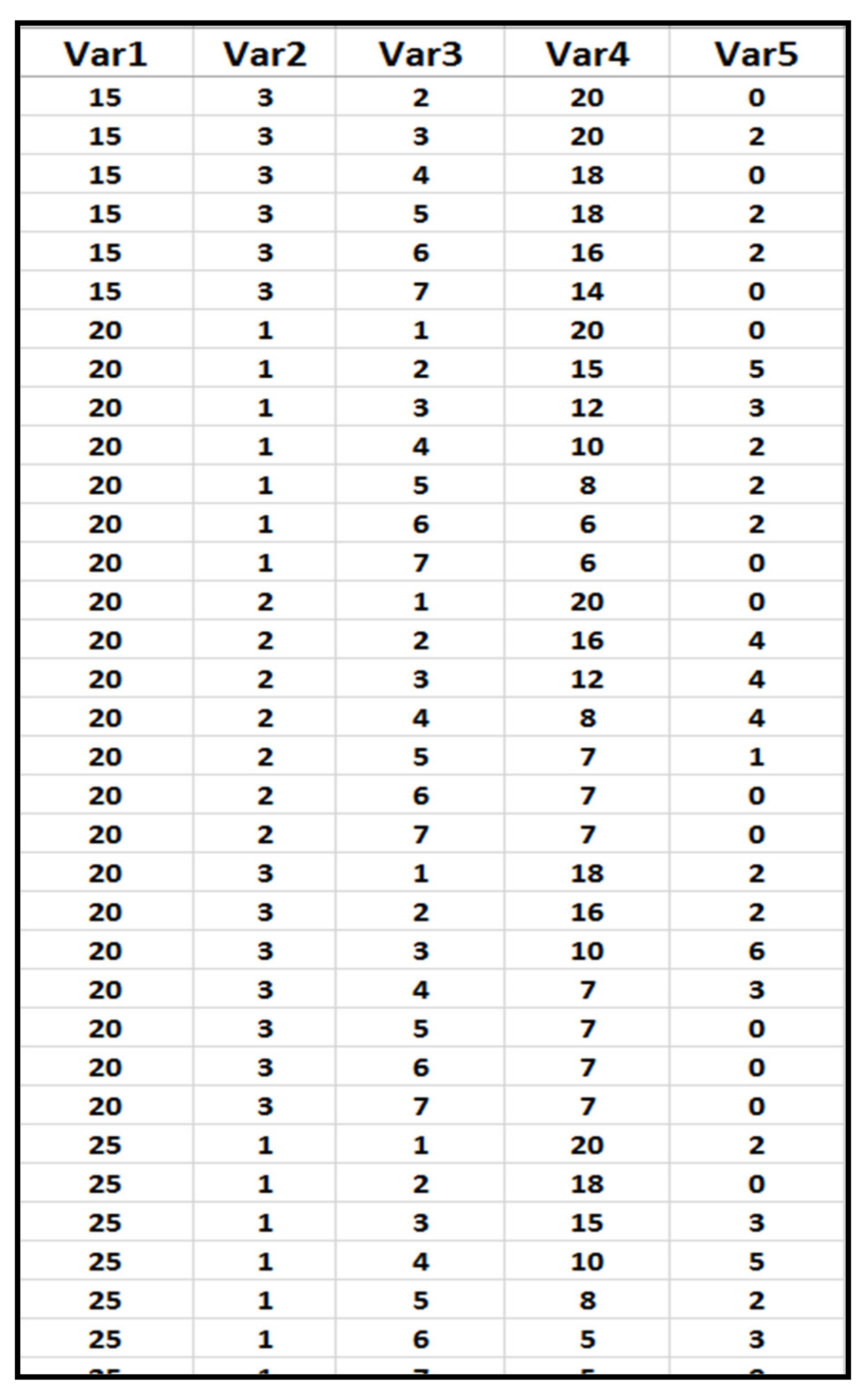
2.1.1. Experimental Data

The fitting process takes, as input, experimental data recorded from observations from the field or laboratory. In the context of biological control used as the case study here, the virulence data have to be obtained from laboratory experiments replicated over a range of different temperatures under which both the insect and the entomopathogen can interact. Data recorded from the experiments are structured and organized per replicate and temperature, then used as inputs to the platform. Temperature was selected as the key variable due to the paramount role it plays in the development, survival, reproduction, and mortality of Entomopathogenic Fungi (EPF) and insects. A time step of hour, day, or week is necessary for each replication, which allows observing changes in the dependent variable (mortality). Records used as input into the platform are structured and organized as presented in Figure A1 (Appendix A).

2.1.2. Climate Data

Climate data are useful during the mapping process and the spatial projection of the model. Data such as temperature of the studied area are extracted from global climate data (http://www.worldclim.org/). These climate layers contain monthly minimum, maximum, and mean temperatures organized in raster files with “Flat” format (.flt and .hdr file), with a spatial resolution ranging from 30 arc-seconds (~1 km) to 10 arc-minutes (~20 km) [19].

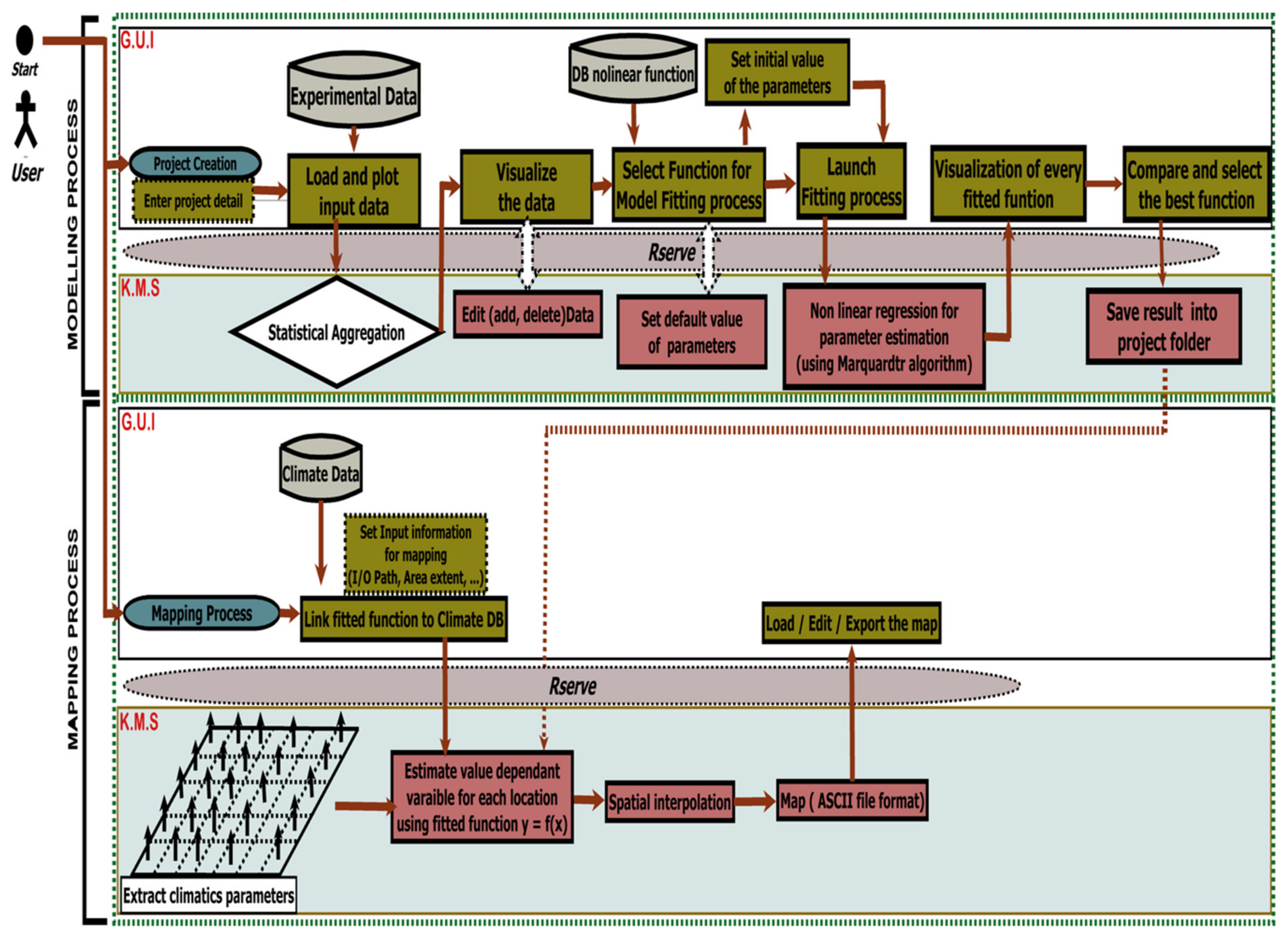
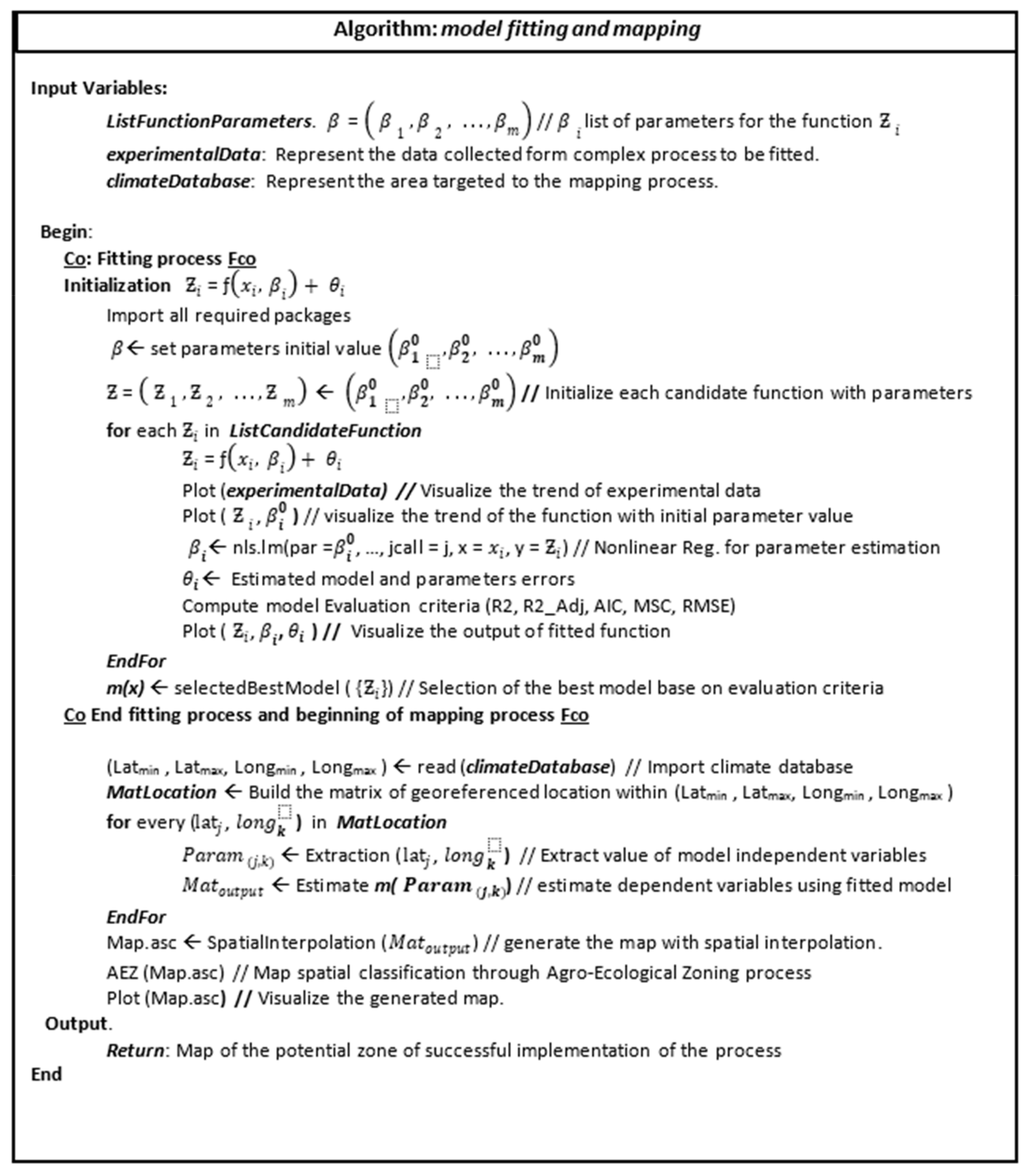
2.2. Model Fitting Description

The model fitting process can be divided into three stages: pre-regression, regression, and post-regression steps [20]. The pre-regression stage mainly consists of the selection of a set of mathematical expressions to be fitted to the data. The regression stage consists of selecting the proper method for parameter estimation, while the post-regression stage consists of sets of activities necessary to evaluate the model.
To illustrate the model fitting process, the following mathematical annotation is used:
z = f x , β + θ ,
where z is the response variable, x represents the input variables, β is the parameter of the model to be estimated, and θ is the error. ƒ is a mathematical function such as an exponential or logarithmic function (see Table 1 for more examples), whose expression depends on x and β. For example, if f is the exponential function with the mathematical expression f ( x ) = b x x b 2 , you have β f = b , x b .
The ability to identify and include the right variables in a model is equally important to the type of model chosen. We consider a group of m observations z i on variables x i and try to estimate parameter β by minimizing θ. The minimization of θ follows the least-square curve-fitting procedure using the Levenberg–Marquardt (LM) algorithm. For a given equation f(x,β), parameters are estimated such that the sum of square of the deviations s β minimizes θ via the following expression: s β = i = 1 m z i f x i | β 2 .
The LM algorithm combines the gradient descent and the Gauss–Newton methods. The gradient descent method reduces the sum of the squared errors by updating the parameters in the downhill direction (the direction opposite to the gradient of the equation), while the Gauss–Newton method reduces the sum of the squared errors by assuming the least-square function is locally quadratic with parameters near the optimum. The fitting procedure starts with an initial value of x0; then, x is adjusted by ∆ only for downhill steps verifying (JTJ + λI) ∆ = JTr, where J is the Jacobian matrix of derivatives of the residuals for the parameters, λ is the damping parameter between the two steps, and r is the residual vector. A set of equations used in the study that can be selected by the user are presented in the Supplementary Materials.
The selection of mathematical expressions for the fitting process is guided by the type of data available to fit, the knowledge of the system, and its boundaries conditions. The estimation of mathematical expression parameters is directly linked to the convergence of the fitting algorithm and the initial conditions [3].

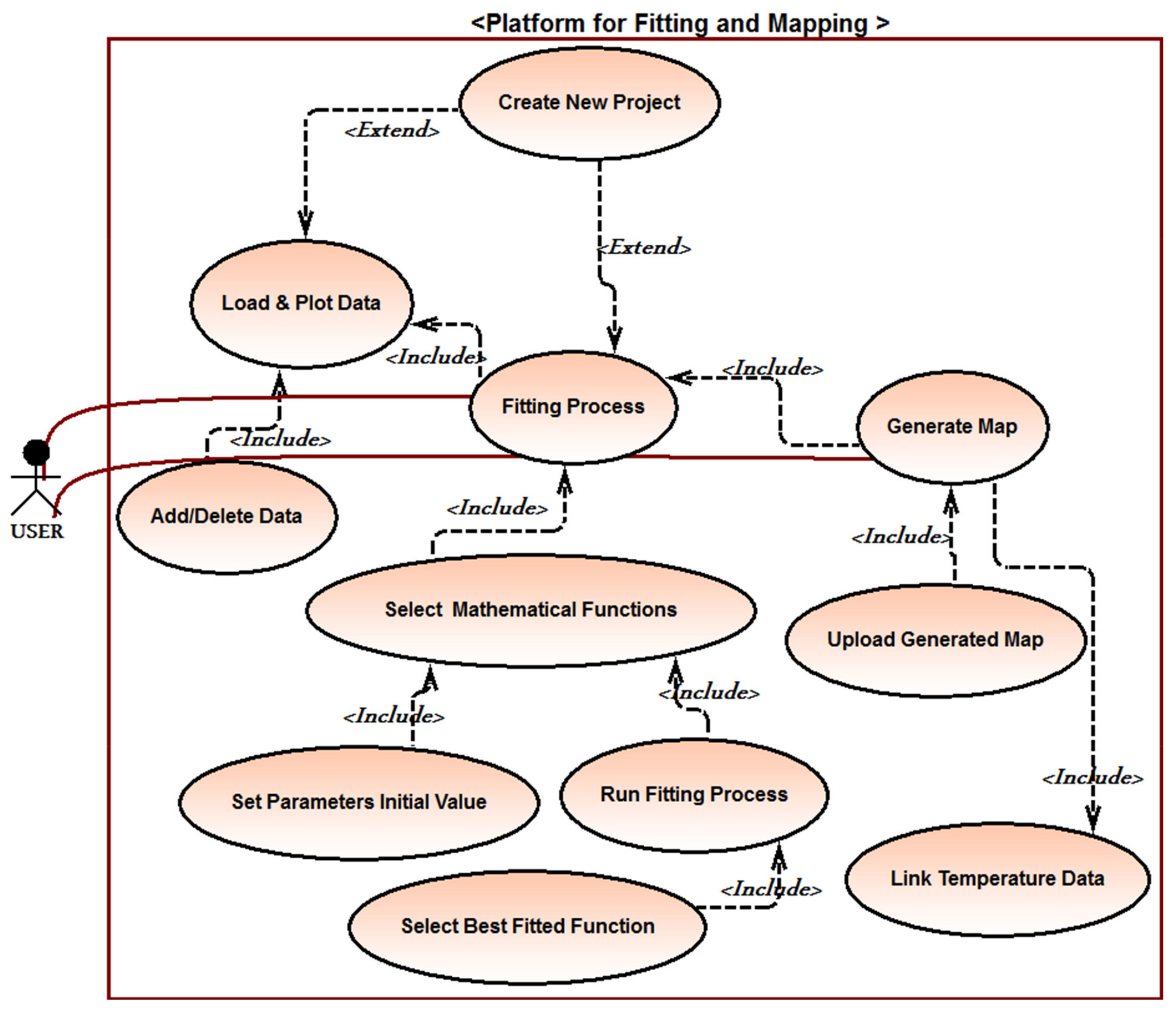
2.3. Features of the DSS

Spatial visualization emerged as the field that combines the abilities of human perception through data picturing and computer simulation using analytics at the landscape level. Spatial visualization was successfully applied in various studies, and the current platform is inspired by these concepts.
The main features of the platform and how they are linked is described in the unified modeling language (UML) use case diagram shown in Figure 1.
The model fitting and mapping process are done through an interactive process that involves the user in all steps to ensure good and reliable decisions are taken, based on graphical outputs and statistical criteria available in the DSS. The process is summarized in Figure 2.
The fitting procedure begins with a preliminary visual display of input data using statistical aggregation functions to provide the average value for all replicates of the experiment. Then, among the 82 nonlinear mathematical expressions, those which can better fit the data are selected. The database of mathematical expressions is obtained from the literature, and each equation is selected based on its ability to capture the relationship that exists between the dependent and the independent variable. The functions used during this process are implemented in R computer language. The implementation of the Levenberg–Marquardt algorithm in R-package minpack.lm is used for fitting the mathematical expressions to data and estimating the parameters [21,22,23]. R-squared, R-squared adjusted, Akaike information criterion (AIC), root-mean-squared error (RMSE). and the sum of squared residual are proposed to help to choose the best-fitted model. Once the fitting process is completed, the information is saved and transferred to the mapping perspective.
The mapping exercise requires spatial data as input, which are organized by grids that allow applying the model at the landscape level. From the graphical user interface (GUI), a request is made to a specific studied region, and the values of temperature in the selected locations are extracted from the database in the form of monthly and annual averages. A point object is used to pick the model mathematical expression, and it is consecutively applied in each geographical coordinate of the region of interest to estimate the value of the dependent variable. This allows the value of the dependent variable at each location to be estimated and stored in an ASCII file format (.asc). Additionally, the mapping perspective includes some Udig features for map editing and viewing. It further offers the possibility to transfer the ASCII file obtained to any geographic information system (GIS) software for processing (see Figure A2, Appendix A, for a summary of the algorithm).

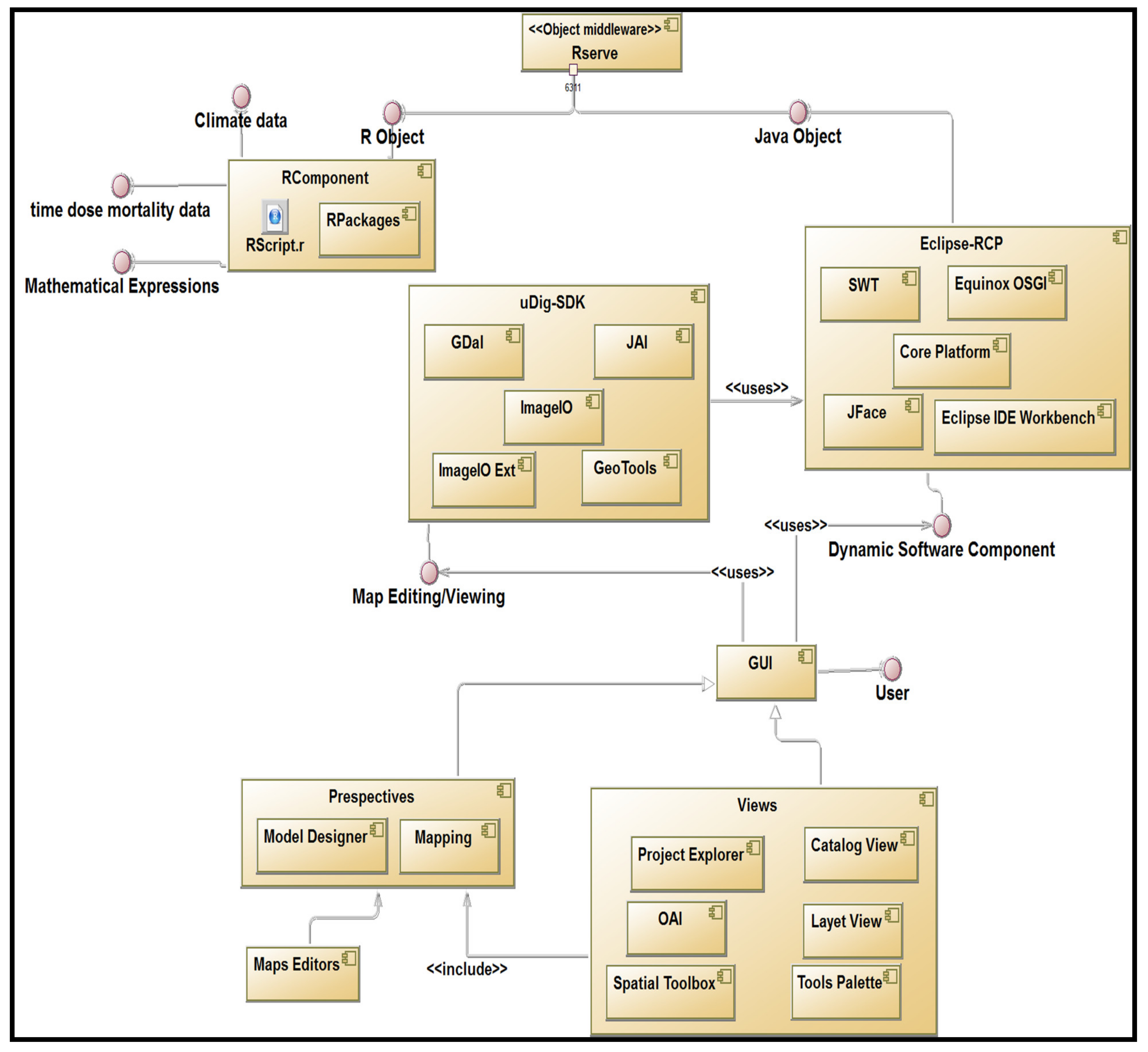
2.4. Software Design and Architecture

The tool is designed using the component-based software architectural approach centered on the Rich Client Platform (RCP) framework. The adopted approach for the software development is proven to simplify and facilitate the productivity and the quality of the end product by enhancing the concepts of software reuse, modularity, extensibility, customization, and reduction of development time [24]. The platform extends all the properties of the Udig framework (Figure 3). Moreover, software developed using RCP can run on a variety of operating systems (e.g., Windows, Linux, or Mac).
The Eclipse integrated development environment (EDI), which is one of the most commonly used tools for the programming of component-based software [24], was used to develop the tool (see “Supplementary Materials” for the link to source code and setup). Eclipse has the advantage that it allows modular and object-oriented programming, which accepts simple development and extension of the tool product [24]. The platform is structured into five major components (see Section 2.4.1, Section 2.4.2, Section 2.4.3, Section 2.4.4 and Section 2.4.5) including the RComponent, Eclipse RCP, Rserve, Udig-SDK, and the graphical user interface (GUI) (Figure 3). A procedural approach is used in RComponent for the fitting of mathematical equations and statistical criteria, while object-oriented programming is used to interconnect all the components and implement the software GUI.

2.4.1. RComponent

RComponent integrates the features to import data, carry out the analytics, and display the results. RComponent consists of R-scripts encompassing the mathematical expressions, fitting algorithms with procedures for equations and parameter estimations, statistical criteria for selection, and the mapping environment. RComponent enables selecting the equation that best fits the data, which is then applied to temperature raster files for spatial projection. Different R packages (minpack.lm, MASS for nonlinear regression and equation fitting; sp, maptools, rgdal, maps, doRNG for spatial operations leading to the creation of the map) are used within RComponent [25,26,27,28,29,30]. The nls.lm() function implemented in the minpack.lm package was used to simulate the Levenberg–Marquardt algorithm. Spatial objects representing climate data are imported using the function readGDAL () from the rgdal package and writeAsciiGrid(), while the maptools package is used to export spatial grid data into ASCII format. Commonly used statistical criteria for comparing and selecting mathematical expressions such as R-squared, R-squared adjusted, Akaike information criterion (AIC), root-mean-squared error (RMSE), and the sum of squared residual (SSR) are implemented into RComponent of the platform.

2.4.2. Eclipse RCP

The Eclipse RCP component enables the building of fast and reliable end-user interfaces to guide users during the interactions with the software functionalities. This component consists of different low-level frameworks that offer ways to rapidly develop client-side applications. The software includes the following key features from the RCP framework: the Equinox OSGI (Open Services Gateway initiative) for describing the modular approach used in Java application under Eclipse; the core platform that contains the runtime engine responsible for the run of plug-ins; the JFace dialog preference and wizard framework; the Standard Widget Toolkit (SWT), which provides objects with subclasses of image, color, and font; the Eclipse IDE workbench. All of these features are used to provide a user-friendly and flexible solution.

2.4.3. Rserve

Rserve is a software component used for the creation of objects and the evaluation of the RComponent scripts, as well as their integration into the Java application [31]. This component is used in the developed tool as an object middleware to enable communication and exchange of information between RComponent and the Eclipse RCP component. It is also called an object request broker, which allows the application to send objects and request responses via object-oriented systems. Once a request is issued, Rserve opens a connection to collect the parameters of the request and establishes another connection with RComponent to provide resources for the execution of the request. When the task is completely executed, the output produced by RComponent is sent back to the GUI.

2.4.4. Udig-SDK

Udig-SDK is an open-source desktop application framework built with Eclipse RCP technology, which can be used as a plug-in in RCP applications. To handle the mapping process, the software extends Udig properties to provide a complete Java solution for desktop geographic information system (GIS) data access, editing, and visualization of maps. It is based on GeoTools, ImageIO-Ext, ImageIO, JAI (Java Advanced Imaging), and Gda; the Udig-SDK component allows the mapping of spatial data. Among the key features offered by Udig for map edition, we have layers, style, (AOI (Area of Interest), and catalog. These features allow the user of the developed tool to add or create layers and customize maps.

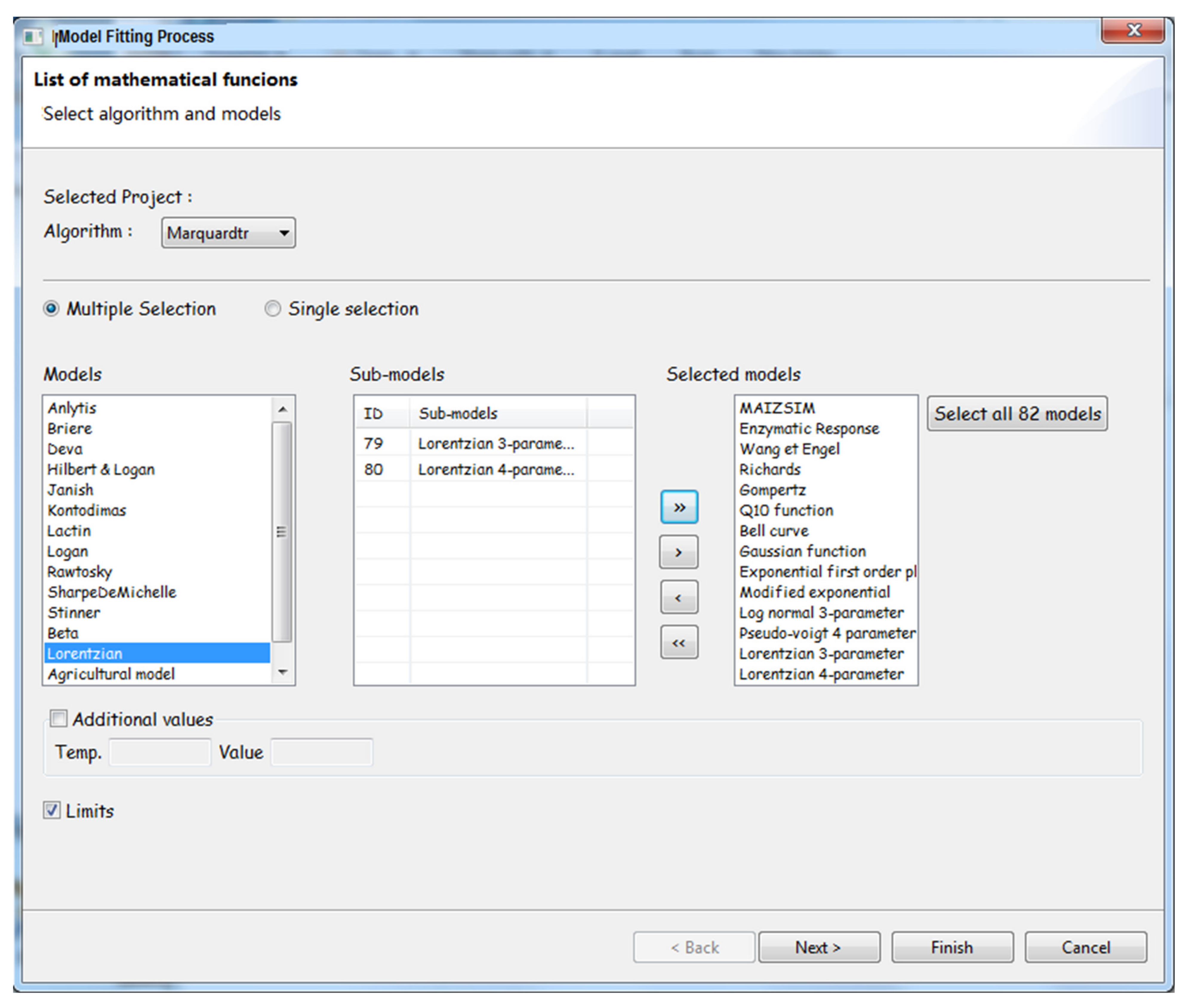
2.4.5. Graphical User Interface (GUI)

This component is the direct link between the user and the software system. Different perspectives are used to bring key functionalities together in a screen layout that is simple and interactive. The software GUI consists of two perspectives: the model designer and the mapping perspective. The model designer displays functionalities needed for the analytics to (i) import, modify, plot, and visualize experimental data, and (ii) carry out equation fitting. The mapping perspective includes all functionalities for the mapping process. Both perspectives include views, a toolbar, a menu bar, and other graphic components needed for a user graphic interface.

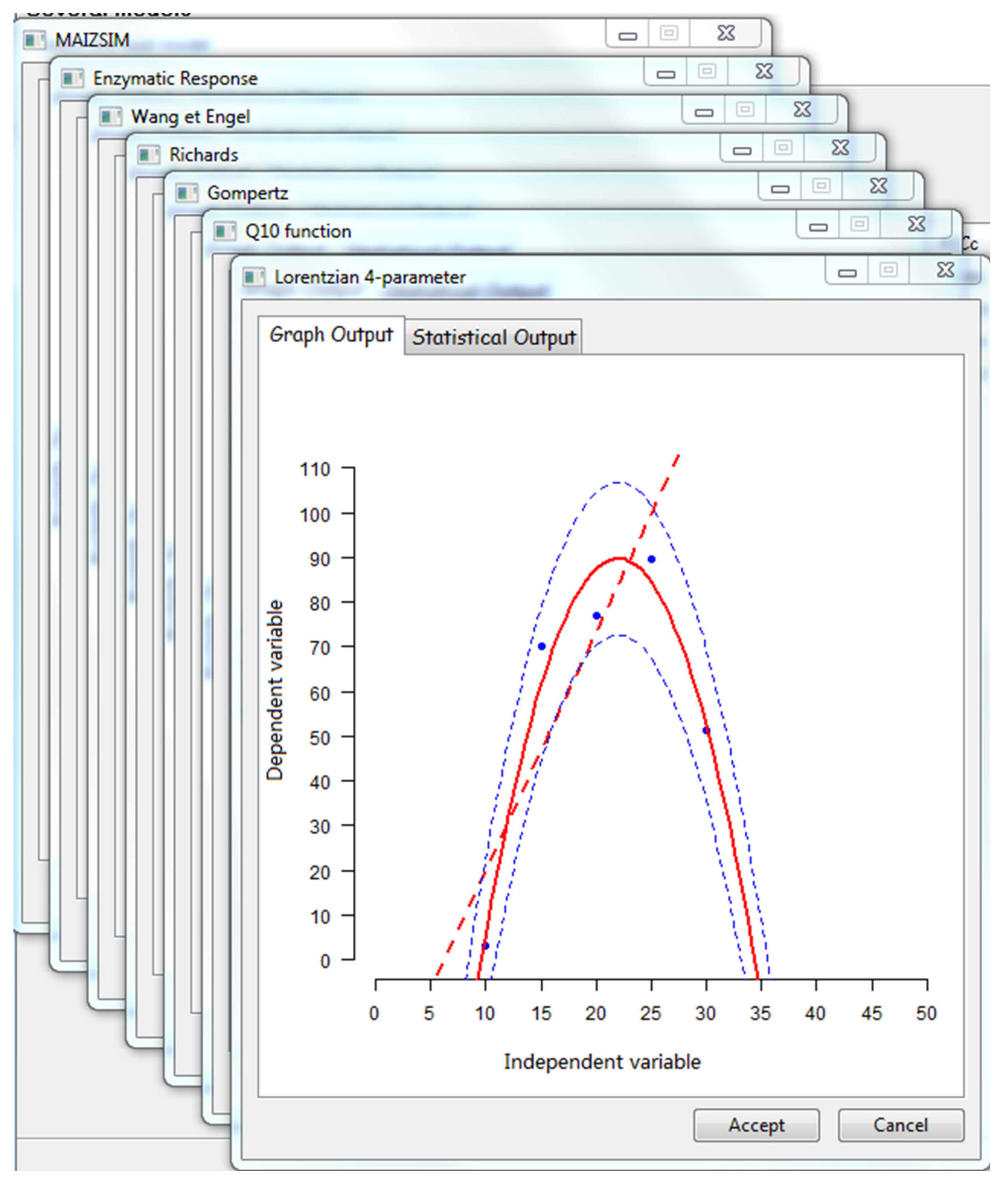
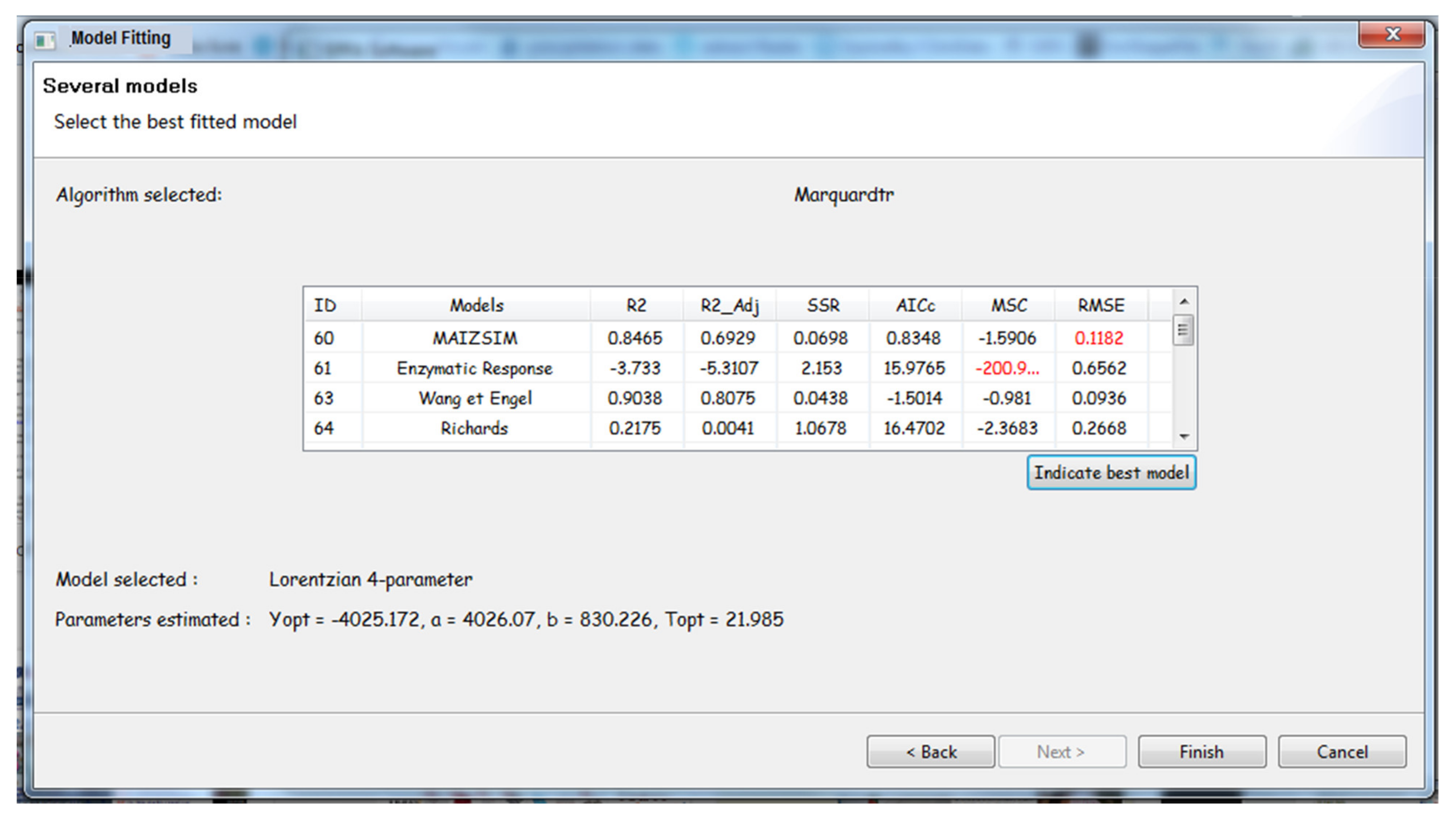
2.4.6. DSS Output Evaluation

The developed DSS produces two main outputs: the model that best fit the experimental data and the geographical distribution map displaying areas of suitability or application of control measures. To evaluate the prediction accuracy of the outputs, users are requested to conduct additional investigations in natural conditions and use the model (if fitted with data from the laboratory) to mimic the field behavior or vice versa. When the output of the DSS is a map, ground scouting is necessary to confirm the projections.

3. Case Study: Using the DSS to Fit Time–Dose–Mortality Data to Mathematical Expressions and Mapping the Potential Zone of Efficacy of Fungal-Based Biopesticides in the Killing of Insect Pests

The case study consisted of using the DSS features to map the potential zone of efficacy for the virulence of the biopesticide Metarhizium anisopliae isolate ICIPE 62 against mustard aphids.
Fungi are the most widespread entomopathogenic organisms in terrestrial ecosystems [32,33], gaining many interest for their potential use as biopesticides, due to their ability to infect and kill insects [32,34,35]. Their efficacies were demonstrated both in laboratories and in the field, leading to a worldwide increasing interest in the development of EPF-derived products for commercialization. They are, however, highly influenced by biotic (e.g., pest dynamics) and abiotic (e.g., sunlight, rainfall, temperature, humidity) factors. The platform is used to fit the time- and temperature-dependent mortality data to temperature-dependent virulence mathematical expressions. Thereafter, the virulence equation that best fitted the data is spatially projected to map the areas of the potential efficacy of the biopesticide in controlling the targeted pest.
Data on the mortality (dependent parameter) of mustard aphids caused by the biopesticide Metarhizium anisopliae isolate ICIPE 62 were obtained in the laboratory at five different temperatures (independent parameter): 10, 15, 20, 25, and 30 °C. Many isolates of Metarhizium anisopliae were reported to have high pathogenicity against several insect pests [36,37,38]. Lipaphis pseudobrassicae, commonly known as turnip aphid or mustard aphid, is a pest that can feed on many types of crops; it was recorded from host plants belonging to over 10 families including Brassicaceae, Cucurbitaceae, and Solanaceae [39]. This pest is globally distributed with the highest level of infestation occurring in Africa, while it is also present in Europe, Asia, and America [40]. The optimal temperature for its development is reported to be around 20 °C [41]. The virulence map was produced for Kenya and Cameroon after completing the fitting process. The spatial evaluation of the generated map was made by comparing the known locations of successful field application of the biopesticide in controlling targeted insect pests to the predicted level of virulence. Illustrations are done below in an interactive way through the features of the designed tool.

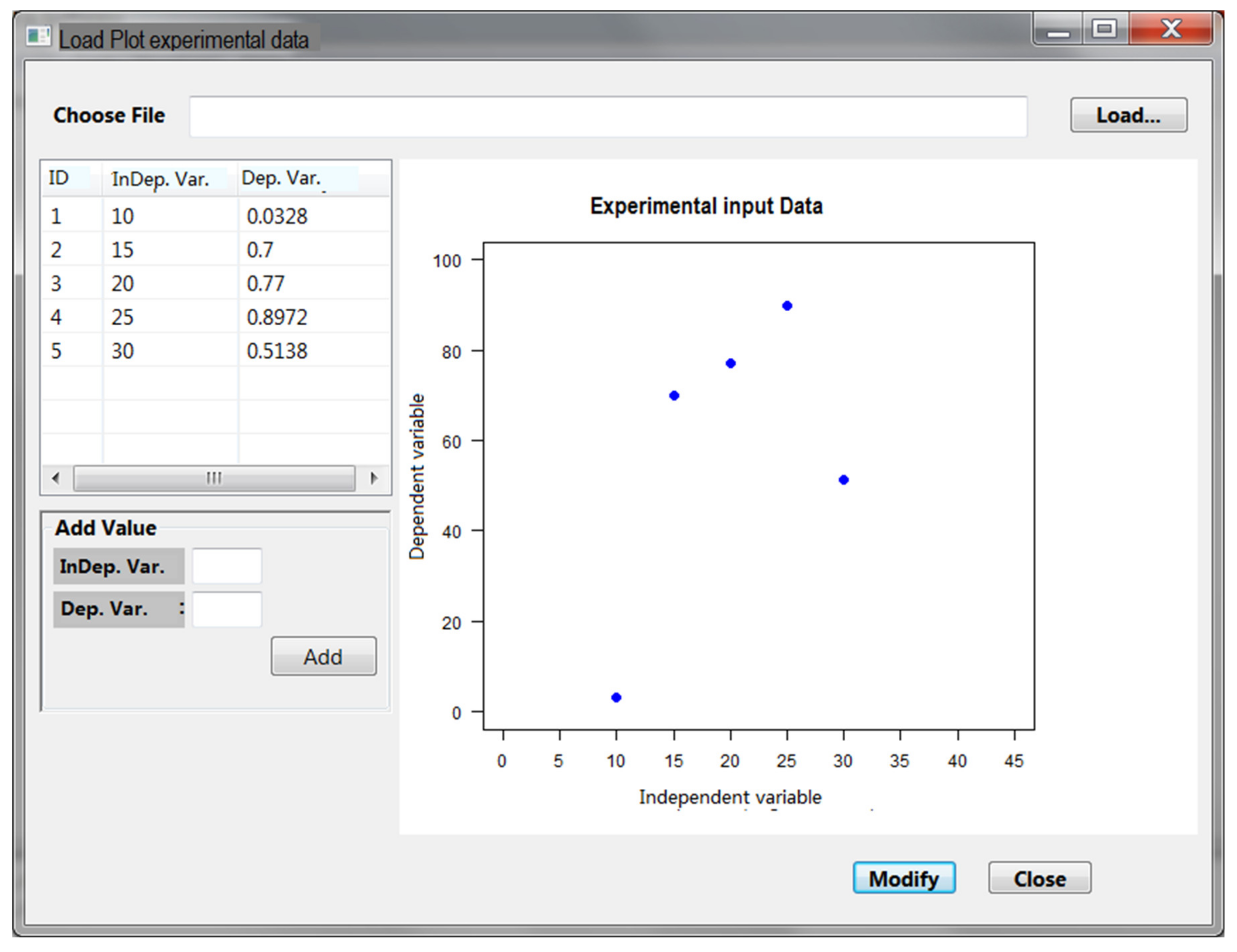
3.1. Data Input, Visualization, and Model Fitting Features

The fitting exercise starts with the creation of a new project using the provision of general information such as the project name and name of the EPF, the name of the author, and a brief description of the project. After the creation of the project, the default display in the environment of the tool is the model designer perspective, which is interactive and intuitive in guiding the user through different steps. The independent and dependent variables, in this case, are temperature and insect mortality due to the interaction with EPF, respectively. For example, the virulence rates of the EPF on the targeted insects at temperatures of 15 and 25 °C are 0.7 and 0.89, respectively (Figure 4). The next step consists of loading the experimental data file, which is displayed in Figure 5 on the left side of the user frame. On the right side of the GUI, the recorded mortality is plotted against the corresponding temperature values (Figure 4). Furthermore, the tool offers the user the possibility to include additional temperature values not included in the initial input data file. The new data could be obtained from the literature.
The user can choose to fit a single or many mathematical equations among the 82 available in the software to the input data (Figure 5).
For each equation selected to be fitted to the data, the graph and statistical parameters are generated and displayed in the user interface (Figure 6). By combining the graphical display of the output with the different values of the goodness of fit (Figure 7), the fitted equation with the best performance is selected as the temperature-dependent virulence model for mapping purposes.

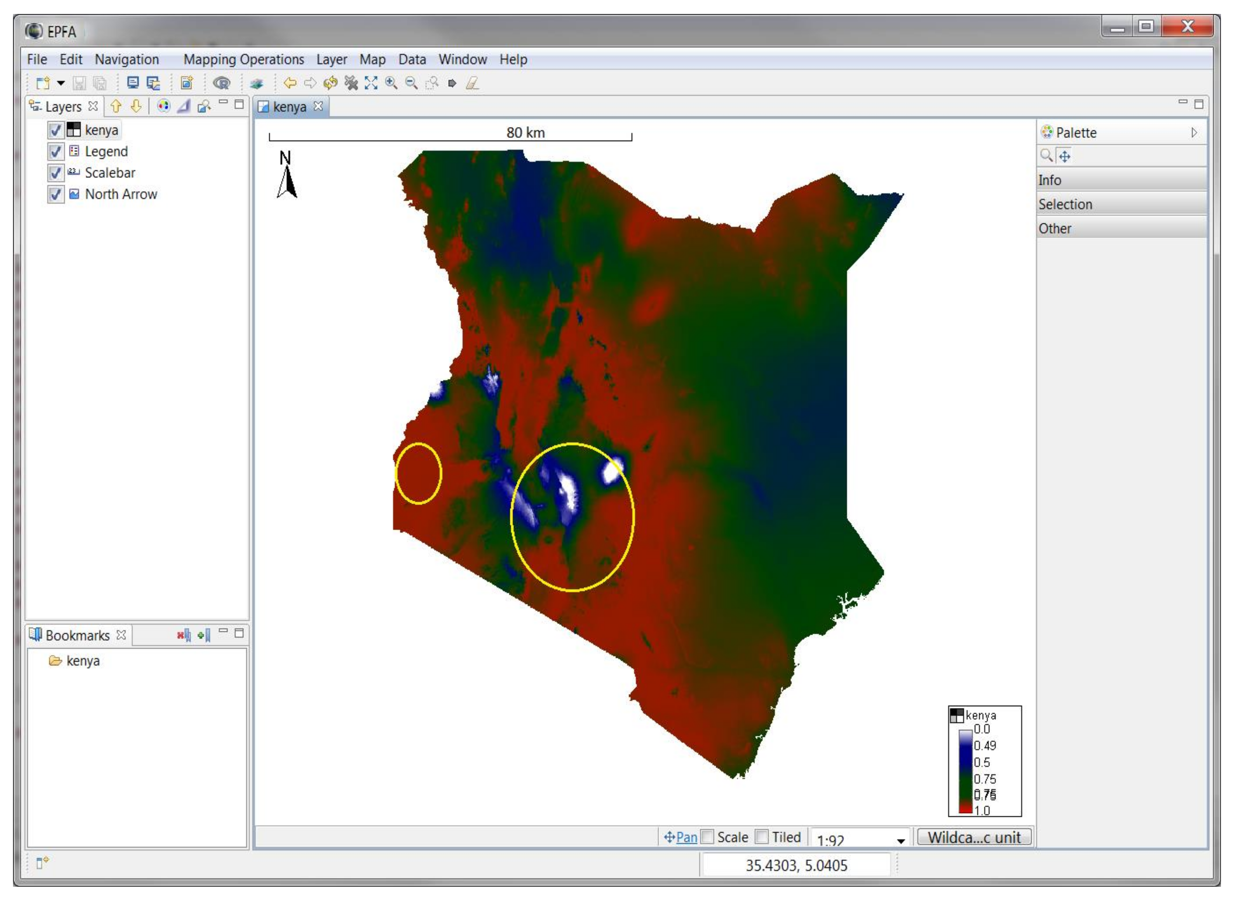
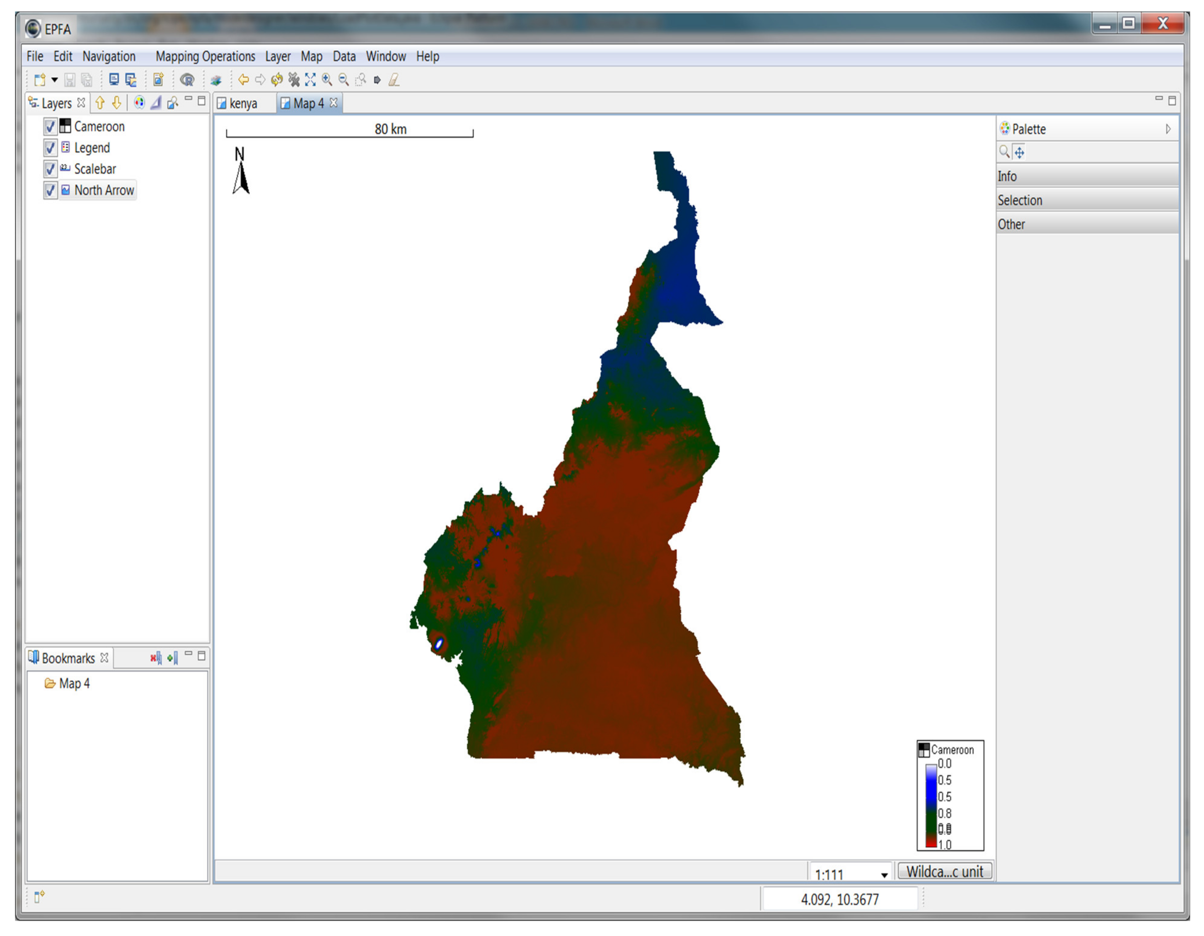
3.2. Mapping Features

Within the mapping perspective, the selected model is linked to climatic data to generate the map (ASCII file) of the potential virulence efficacy. Layers for minimum and maximum temperatures can be imported, and the extent of the area of interest can be defined. Optionally, a filter can be applied to limit the minimum and maximum temperature values that are considered suitable for the process. After the model is linked with a climatic database, a map is produced through a spatial interpolation technique. The user has the option to use the features provided through Udig for additional editing and layouts of the efficacy map or to transfer the generated ASCII file to another GIS software such as QGIS.
The results considered in the case study indicate that the optimum temperature to apply the EPF isolate ICIPE 62 with the highest level of virulence is 22 °C (Topt = 21.98 °C ± 0.29). Based on the Lorentzian four-parameter model results, the maps of the potential zones of the efficacy of EPF isolate ICIPE 62 when applied against mustard aphid were produced for Kenya and Cameroon (Figure 8 and Figure 9, respectively). A level of efficacy that varies between 0 and 1 characterizes the virulence level of ICIPE 62 against the targeted pest.
Locations with a virulence level of efficacy ranging from 0 to 0.5 are locations with an average environmental temperature below 15 °C. Locations with a virulence level of efficacy ranging from 0.5 to 0.8 are locations with an average environmental temperature varying from 15 °C to 17 °C and from 26 °C to 30 °C. Locations with a virulence level of efficacy ranging from 0.8 to 1 correspond to locations with an average environmental temperature varying from 17 °C to 26 °C.
To evaluate the prediction accuracy of the output map, field releases of the EFP were conducted at the point locations circled in Figure 8. The outcome, which was a successful control measure, is compared with the model-predicted level of virulence that is greater than or equal to 50%.

4. Discussion

This paper presented the design and implementation of an interactive platform for fitting experimental data to mathematical expressions and generating the spatial projection of the result at the local, regional, and continental scales. The platform was developed with the combination of R programming language, RCP architecture, and Udig, which makes it an interactive decision support tool with multiple components, as described in the literature [12,13,14]. The most important components of the platform are RComponent and the graphical user interface (GUI). However, the trigger of the iterative procedure is the acquisition of the experimental data used as input.
The fitting procedure implemented in the platform applied the LM algorithm. The LM algorithm combines two approaches; it operates like the gradient descent method when the equation parameters are far from their optimal values, while it performs like the Gauss–Newton method when the parameter values are close to their optimum (Nelles, 2001). The main advantage of the LM algorithm is its ability to converge to optimum values faster than the gradient descent or the Gauss–Newton method. This allows the LM algorithm to still find the optimal value of parameters when the initial values of equation parameters are distant from the optimum. This makes the LM algorithm very robust when compared to other minimization algorithms usually used in the fitting procedure (Nelles, 2001).
The GUI is considered as a key component of the tool as it is used directly by the end-user to interact and communicate with the system. The design of the software GUI satisfies the requirements for a software development interface as described in Reference [42]. The component-based approach is adopted to rely on the possibilities to extend and reuse developed components. By employing such a development concept, the maintenance of the software architecture can be secured while new functionalities can be easily integrated. Component-based UIs further enable functional and logical decomposition of the software GUI into perspectives, which helps in defining features needed by the end-users. Component-based UIs accelerate the development process, which is contrary to the iterative or agile development approach that tends to slow the process of developing software. The modularity offered by the RCP component allows easily integrating additional features in the tool.
In comparison to other fields such as education or finance, the need for such tools in agriculture and IPM research activities is lacking despite their importance. This is particularly required to assist in monitoring numerous processes in the crop production system, such as field release of biological control agents. In recent years, progress was perceptible with the proliferation of DSS [43,44], which can be web-based [43] or standalone like the proposed DSS. Despite disparities among conceptual approaches, what they all have in common is the emphases put on input data and the user interface. One advantage of a web-based DSS is the possibility it offers to directly access real-time environmental data to carry out analytics [44], which make these categories of tools highly dependent on an internet connection that is not always available in most of Africa. A standalone DSS, once installed, only requires acquiring input data to be used anywhere and offline. Moreover, the uniqueness of this tool is the flexibility it offers to easily provide spatial distribution maps using gridded values of temperature for delimiting potential areas of field application of control measures. A similar attempt was presented in References [45,46]; however, it is not directly applicable as users still need to be knowledgeable in statistical and geospatial sciences. The current platform generalizes and combines all the steps used in these studies to provide researchers, with no computational skills, the opportunity to process the fitting and select the models that can further be projected spatially at the landscape level.
Application: The Lorentzian 4-parameter model obtained in the application section estimates an optimum temperature for the higher virulence of ICIPE62 in killing the aphid at about 21 °C. When comparing the current distribution map of the Lipaphis pseudobrassicae [40] with the map of the potential zone of the efficacy of ICIPE 62 isolate in Kenya and Cameroon, we observed that many invaded locations fit well with a potential zone of efficacy with virulence level greater than or equal to 0.5. Although the estimates were made without full inclusion of other environmental variables that have impacts on the fungi efficacy in killing insects, the outputs are promising. However, it will be useful to explore the association of temperature with other factors such as relative humidity to improve the accuracy of the prediction, especially for mapping the virulence level of the EPF. Indeed, many studies highlighted the key role played by both temperature and relative humidity in enhancing the virulence of EPF on insect pests [47,48,49]. On this note, a good perspective to consider for improving the current tool will be to consider the association of at least two factors (temperature and relative humidity, for example) as independent variables in the fitting process.

5. Conclusions and Future Works

Herein, we presented an interactive generic platform for predicting agro-ecological processes through the use of experimental data that are fitted to mathematical expressions, whereby the resulting best-fitted equation can be applied at the landscape level. The platform is a useful tool for anyone interested in fitting and conducting a spatial visualization of data. The current platform could be of great help for science pathologists and IPM practitioners worldwide in their attempt to increase the use and application of control measures within an agriculture IPM context. To further improve DSS development, the economic injury level (EIL) concepts that rely on economic threshold models may be added as a guide in evaluating the cost and benefit of deploying any control measure. The added module will integrate a combination of environmental and biological factors which are linked to economic factors, yielding an environmental economic threshold module. However, to avoid complexity, it is also possible that outputs from the developed tool can be used as input in other software specifically developed to conduct econometric analysis.

Supplementary Materials

The source code of the software is available online at https://github.com/Atoundem/EPFA_RCP. The setup and installation requirements can be downloaded at https://github.com/Atoundem/EPFA_RCP/tree/master/Setup_Intall_Requirement.

Author Contributions

Conceptualization, S.E. and H.E.T.; Methodology, R.A.G. and H.E.Z.T.; Software, R.A.G. and H.E.Z.T.; Writing—original draft preparation, R.A.G.; Writing—review and editing, R.A.G., L.B.-F., C.B. and H.E.Z.T.; Supervision, S.A.M., W.M. and H.E.Z.T.; Funding acquisition, S.E. and H.E.Z.T. All authors have read and agreed to the published version of the manuscript.

Funding

This work was supported by the Volkswagen Foundation under Grant [VW-94362].

Acknowledgments

The first author of this study is a PhD student working in the fellowship project (VW-89362) of Henri E.Z. Tonnang funded by the Volkswagen Foundation under the funding initiative Knowledge for Tomorrow: Cooperative Research Projects in Sub-Saharan on Resources, their Dynamics, and Sustainability—Capacity Development in Comparative and Integrated Approaches. The authors thank the Federal Ministry for Economic Cooperation and Development (BMZ), Germany, which provided the financial support through the Tuta IPM project, the German Academic Exchange Service (DAAD), and the STRIVE project funded by the German Federal Ministry of Education and Research.

Conflicts of Interest

The authors declare no conflict of interest.

Appendix A

Figure A1. Experimental data: Var1 represents the range of the independent variable (temperature); Var2 is the number of replicates in the experiment, Var3 is the time duration of each experiment; Var4 and Var5 are records of the dependent variable (mortality) with the variation of the independent variable.
Algorithms 13 00104 g0a1
Figure A2. Algorithm: model fitting and mapping processes.
Algorithms 13 00104 g0a2

References

  1. Jones, J.W.; Antle, J.M.; Basso, B.; Boote, K.J.; Conant, R.T.; Foster, I.; Godfray, H.C.J.; Herrero, M.; Howitt, R.E.; Janssen, S.; et al. Brief history of agricultural systems modeling. Agric. Syst. 2017, 155, 240–254. [Google Scholar] [CrossRef] [PubMed]
  2. Lepenioti, K.; Bousdekis, A.; Apostolou, D.; Mentzas, G. Prescriptive analytics: Literature review and research challenges. Int. J. Inf. Manag. 2020, 50, 57–70. [Google Scholar] [CrossRef]
  3. Archontoulis, S.V.; Miguez, F.E. Nonlinear Regression Models and Applications in Agricultural Research. Agron. J. 2015, 107, 786. [Google Scholar] [CrossRef] [Green Version]
  4. Klosterman, R.E. Simple and Complex Models. Environ. Plan. B Plan. Des. 2012, 39, 1–6. [Google Scholar] [CrossRef]
  5. Eva, Y.-H.; Wu, M.-C. Hung, Comparison of Spatial Interpolation Techniques Using Visualization and Quantitative Assessment. Appl. Spat. Stat. 2016, 11, 17–34. [Google Scholar] [CrossRef] [Green Version]
  6. Patel, N.R.; Mandal, U.K.; Pande, L.M. Agro-ecological Zoning System-A Remote Sensing and GIS Perspective Upscaling of photosynthesis through Sun-induced fluorescence (SIF) View project 1. Regional Carbon Cycle Modeling for India and surrounding oceans View project. J. Agrometeorol. 2000, 2, 1–13. Available online: https://www.researchgate.net/publication/270683979 (accessed on 3 April 2020).
  7. Gimond, M. Intro to GIS and Spatial Analysis. 2019. Available online: https://mgimond.github.io/Spatial/index.html (accessed on 9 October 2019).
  8. FAO. Agro-Ecological Zoning: Guidelines, Rome. 1996. Available online: https://books.google.com/books?hl=fr&lr=&id=IWFD2zGLyrYC&oi=fnd&pg=PA1&dq=AGRO-ECOLOGICAL+ZONING+Guidelines&ots=bAH-Or-Nn0&sig=XdhPDm3WBbN8ckFjP2d5Zj5qaIc (accessed on 3 April 2020).
  9. Mardani, A.; Jusoh, A.; Nor, K.M.D.; Khalifah, Z.; Zakwan, N.; Valipour, A. Multiple criteria decision-making techniques and their applications—A review of the literature from 2000 to 2014. Econ. Res. Istraž. 2015, 28, 516–571. [Google Scholar] [CrossRef]
  10. Belton, V.; Stewart, T.J. Multiple Criteria Decision Analysis: An Integrated Approach; Springer: New York, NY, USA, 2002. [Google Scholar]
  11. Stojčić, M.; Zavadskas, E.; Pamučar, D.; Stević, Ž.; Mardani, A. Application of MCDM Methods in Sustainability Engineering: A Literature Review 2008–2018. Symmetry (Basel) 2019, 11, 350. [Google Scholar] [CrossRef] [Green Version]
  12. Sprague, R.H.; Carlson, E. Building Effective Decision Support Systems; Prentice Hall College Div: Englewood Cliffs, NJ, USA, 1982. [Google Scholar]
  13. Dan, P. Ask Dan about DSS—What Are the Components of A Decision Support System? 2005. Available online: http://dssresources.com/faq/index.php?action=artikel&id=101 (accessed on 5 April 2017).
  14. Karacapilidis, N. An Overview of Future Challenges of Decision Support Technologies; Springer: London, UK, 2006; pp. 385–399. [Google Scholar] [CrossRef] [Green Version]
  15. Huber, G.P. Organizational science contributions to the design of decision support systems. 1980. Available online: http://pure.iiasa.ac.at/id/eprint/1221/1/XB-80-512.pdf#page=55 (accessed on 17 January 2020).
  16. Fick, G.; Sprague, R.H. Decision Support Systems: Issues and Challenges: Proceedings of the an International Task Force Meeting June 23–25, 1980; Elsevier: Oxford, UK, 1980. Available online: http://www.sciencedirect.com/science/book/9780080273211 (accessed on 5 April 2017).
  17. Wierzbicki, A.P.; Makowski, M.; Wessels, J. Model-Based Decision Support Methodology with Environmental Applications. Interfaces 2000, 32(2), 84. [Google Scholar] [CrossRef]
  18. Power, D.J. Understanding Data-Driven Decision Support Systems. Inf. Syst. Manag. 2008, 25, 149–154. [Google Scholar] [CrossRef]
  19. Hijmans, R.J.; Cameron, S.E.; Parra, J.L.; Jones, P.G.; Jarvis, A. Very high resolution interpolated climate surfaces for global land areas. Int. J. Climatol. 2005, 25, 1965–1978. [Google Scholar] [CrossRef]
  20. Jaqaman, K.; Danuser, G. Linking data to models: Data regression. Nat. Rev. Mol. Cell Biol. 2006, 7, 813–819. [Google Scholar] [CrossRef] [PubMed]
  21. Marquardt, D. An Algorithm for Least-Squares Estimation of Nonlinear Parameters. J. Soc. Ind. Appl. Math. 1963, 11, 431–441. [Google Scholar] [CrossRef]
  22. Gavin, H. The Levenberg-Marquardt method for nonlinear least squares curve-fitting problems. 2011. Available online: http://people.duke.edu/~hpgavin/ce281/lm.pdf (accessed on 5 December 2019).
  23. Lourakis, M.I.A. A Brief Description of the Levenberg-Marquardt Algorithm Implemened by levmar. Found. Res. Technol. 2005, 4, 1–6. [Google Scholar] [CrossRef]
  24. Silva, V. Practical Eclipse Rich Client Platform Projects; Apress: New York, NY, USA, 2009. [Google Scholar] [CrossRef]
  25. Gaujoux, R. doRNG: Generic Reproducible Parallel Backend for “Foreach” Loops. 2017. Available online: https://cran.r-project.org/web/packages/doRNG/index.html (accessed on 9 October 2017).
  26. Pebesma, E.; Bivand, R.; Rowlingson, B.; Gomez-Rubio, V.; Hijmans, R.; Sumner, M.; MacQueen, D.; Lemon, J.; O’Brien, J. sp: Classes and Methods for Spatial Data. 2017. Available online: https://cran.r-project.org/web/packages/sp/index.html (accessed on 9 October 2017).
  27. Ripley, B.; Venables, B.; Bates, D.M.; Hornik, K.; Gebhardt, A.; Firth, D. MASS: Support Functions and Datasets for Venables and Ripley’s MASS. 2017. Available online: https://cran.r-project.org/web/packages/MASS/index.html (accessed on 9 October 2017).
  28. Elzhov, T.V.; Mullen, K.M.; Spiess, A.-N.; Bolker, B. Minpack.lm: R Interface to the Levenberg-Marquardt Nonlinear Least-Squares Algorithm Found in MINPACK, Plus Support for Bounds. 2016. Available online: https://cran.r-project.org/web/packages/minpack.lm/index.html (accessed on 9 October 2017).
  29. Bivand, R.; Lewin-Koh, N.; Pebesma, E.; Archer, E.; Baddeley, A.; Bearman, N.; Bibiko, H.-J.; Brey, S.; Callahan, J.; Carrillo, G.; et al. Maptools: Tools for Reading and Handling Spatial Objects. 2017. Available online: https://cran.r-project.org/web/packages/maptools/index.html (accessed on 9 October 2017).
  30. Becker, R.A.; Wilks, A.R.; Brownrigg, R.; Minka, T.P.; Deckmyn, A. Maps: Draw Geographical Maps. 2017. Available online: https://cran.r-project.org/web/packages/maps/index.html (accessed on 9 October 2017).
  31. Urbanek, S. Rserve—A Fast Way to Provide R Functionality to Applications. 2003. Available online: https://www.r-project.org/conferences/DSC-2003/Proceedings/Urbanek.pdf (accessed on 14 April 2017).
  32. Augustyniuk-Kram, A.; Kram, K.J. Entomopathogenic Fungi as an Important Natural Regulator of Insect Outbreaks in Forests (Review). 2012. Available online: https://www.intechopen.com/books/forest-ecosystems-more-than-just-trees/entomopathogenic-fungi-as-an-important-natural-regulator-of-insect-outbreaks-in-forests-review- (accessed on 21 September 2016).
  33. Lacey, L.A.; Grzywacz, D.; Shapiro-Ilan, D.I.; Frutos, R.; Brownbridge, M.; Goettel, M.S. Insect pathogens as biological control agents: Back to the future. J. Invertebr. Pathol. 2015, 132, 1–41. [Google Scholar] [CrossRef] [Green Version]
  34. Roberts, D.W.; Humber, R.A. Entomogenous Fungi. Biol. Conidial Fungi 1981, 2(201), 201–236. Available online: http://linkinghub.elsevier.com/retrieve/pii/B9780121795023500145 (accessed on 21 September 2016).
  35. Shahid, A.A.; Rao, A.Q.; Bakhsh, A.; Husnain, T. Entomopathogenic fungi as biological controllers: New insights into their virulence and pathogenicity. 2012. Available online: http://agris.fao.org/agris-search/search.do?recordID=RS2012000992 (accessed on 21 September 2016).
  36. Bayissa, W.; Ekesi, S.; Mohamed, S.A.; Kaaya, G.P.; Wagacha, J.M.; Hanna, R.; Maniania, N.K. Selection of fungal isolates for virulence against three aphid pest species of crucifers and okra. J. Pest Sci. 2004, 90, 355–368. [Google Scholar] [CrossRef]
  37. Migiro, L.N.; Maniania, N.K.; Chabi-Olaye, A.; Vandenberg, J. Pathogenicity of Entomopathogenic Fungi Metarhizium anisopliae and Beauveria bassiana (Hypocreales: Clavicipitaceae) Isolates to the Adult Pea Leafminer (Diptera: Agromyzidae) and Prospects of an Autoinoculation Device for Infection in the Field. Environ. Entomol. 2010, 39, 468–475. [Google Scholar] [CrossRef] [Green Version]
  38. Niassy, S.; Maniania, N.K.; Subramanian, S.; Gitonga, M.L.; Maranga, R.; Obonyo, A.B.; Ekesi, S. Compatibility of Metarhizium anisopliae isolate ICIPE 69 with agrochemicals used in French bean production. Int. J. Pest Manag. 2012, 58, 131–137. [Google Scholar] [CrossRef]
  39. Akhtar, K.U.S.; Dey, D. Spatial Distribution of Mustard Aphid Lipaphis erysimi (Kaltenbach) Vis-à-vis its Parasitoid, Diaeretiella rapae (M’intosh). World Appl. Sci. 2010, 11, 284–288. [Google Scholar]
  40. CABI. Mustard Aphid (Lipaphis Erysimi) Plantwise Technical Factsheet, Plantwise Knowledge Bank. 2020. Available online: http://www.plantwise.org/KnowledgeBank/Datasheet.aspx?dsid=30913 (accessed on 20 June 2017).
  41. Awaneesh, Mustard Aphid agropedia. 2009. Available online: http://agropedia.iitk.ac.in/node/4578 (accessed on 29 June 2017).
  42. Scott, D. 6 Reasons for Component-based UI Development. 2016. Available online: https://www.tandemseven.com/technology/6-reasons-component-based-ui-development/ (accessed on 14 July 2017).
  43. Jones, V.P.; Brunner, J.F.; Grove, G.G.; Petit, B.; Tangren, G.V.; Jones, W.E. A web-based decision support system to enhance IPM programs in Washington tree fruit. Pest Manag. Sci. 2010, 66(6), 587–595. [Google Scholar] [CrossRef] [PubMed]
  44. Damos, P. Modular structure of web-based decision support systems for integrated pest management: A review. Agron. Sustain. Dev. 2015, 35, 1347–1372. [Google Scholar] [CrossRef] [Green Version]
  45. Klass, J.I.; Blanford, S.; Thomas, M.B. Use of a geographic information system to explore spatial variation in pathogen virulence and the implications for biological control of locusts and grasshoppers. Agric. For. Entomol. 2007, 9, 201–208. [Google Scholar] [CrossRef]
  46. Klass, J.I.; Blanford, S.; Thomas, M.B. Development of a model for evaluating the effects of environmental temperature and thermal behaviour on biological control of locusts and grasshoppers using pathogens. Agric. For. Entomol. 2007, 9, 189–199. [Google Scholar] [CrossRef]
  47. Mishra, S.; Kumar, P.; Malik, A. Effect of temperature and humidity on pathogenicity of native Beauveria bassiana isolate against Musca domestica L. J. Parasit. Dis. 2015, 39, 697–704. [Google Scholar] [CrossRef] [PubMed] [Green Version]
  48. Hsiao, W.-F.; Bidochka, M.J.; Khachatourians, G.G. Effect of temperature and relative humidity on the virulence of the entomopathogenic fungus, Verticillium lecanii, toward the oat-bird berry aphid, Rhopalosiphum padi (Hom., Aphididae). J. Appl. Entomol. 1992, 114, 484–490. [Google Scholar] [CrossRef]
  49. Athanassiou, C.G.; Kavallieratos, N.G.; Rumbos, C.I.; Kontodimas, D.C. Influence of Temperature and Relative Humidity on the Insecticidal Efficacy of Metarhizium anisopliae against Larvae of Ephestia kuehniella (Lepidoptera: Pyralidae) on Wheat. J. Insect Sci. 2017, 17, 22. [Google Scholar] [CrossRef]
Figure 1. Use case diagram presenting the interactions among the platform components and their functionalities. Each circle represents a feature implemented within the decision support system (DSS). The links from the user to a feature represent the direct interactions of the user with the DSS, while the arrows with labels “include” characterize the relationships and level of dependency between features.
Algorithms 13 00104 g001
Figure 2. Detailed flowchart diagram of the platform; the figure displays two processes: the fitting process in which experimental data are fitted to nonlinear mathematical expressions using the Marquardt optimization algorithm and the mapping process that begins by linking the obtained best-fitted model to the climate database for map creation. The GUI represents the graphical user interface, and the KMS is the knowledge management system that processes all the simulations.
Algorithms 13 00104 g002
Figure 3. Unified modeling language (UML) component diagram. The users interact with the inbuilt software environment through the perspectives (model designer and mapping perspective) of the GUI. The GUI is based on the Eclipse-RCP (Rich Client Platform) and Udig-RCP components. Rserve allows the communication between R and Java by creating objects with port 6311.
Algorithms 13 00104 g003
Figure 4. User interface (UI) for importing, plotting, and modifying experimental data.
Algorithms 13 00104 g004
Figure 5. Wizard for the selection list for the fitting process. This frame assists the user in the selection of equations to be fitted with experimental data.
Algorithms 13 00104 g005
Figure 6. Display of all the fitted equations for the selection of the model.
Algorithms 13 00104 g006
Figure 7. Evaluation criteria and goodness of fit for each fitted equation. Cells in red suggest the best-performing function for each evaluation criterion.
Algorithms 13 00104 g007
Figure 8. Kenyan map of the potential efficacy of ICIPE 62 isolate when used against mustard aphid, modeled with the software. The level of efficacy varies between 0 and 1. Locations with 0% level of efficacy are displayed in white, values between 0 and 0.5 are displayed in blue, values between 0.5 and 0.75 are displayed in green, and values between 0.75 and 1 are displayed in red. Red indicates the highest efficacy levels. The yellow circles surround areas in Kenya where the EPF isolate ICIPE 62 is successfully used, and results were used for validation of the developed model.
Algorithms 13 00104 g008
Figure 9. Cameroon map of the potential efficacy of ICIPE 62 isolate when used against mustard aphid, modeled with the software. The level of efficacy varies between 0 and 1. Locations with 0% level of efficacy are displayed in white, values between 0 and 0.5 are displayed in blue, values between 0.5 and 0.75 are displayed in green, and values between 0.75 and 1 are displayed in red. Red indicates the highest efficacy levels.
Algorithms 13 00104 g009
Table 1. Summary of key functions used for fitting. The “Name” column gives the name of the model, the “Equation” column gives the mathematical expression of the model, the “comment” column gives the number of derived sub-models from the original main model, and the last column gives the reference for the model. T is the independent variable, and m(T) represents the virulence model. ID—identifier.
IDModel NameModel Main Mathematical ExpressionCommentReference
1Sharpe and DeMichele m T = p . T T 0 . e Δ H A R 1 T 0 1 T 1 + e Δ H L R 1 T L 1 T + e Δ H H R 1 T H 1 T 12 sub-modelsSharpe and DeMichele 1977
Sharpe and DeMichele 1–13
2Deva m ( T ) = b T T min T ≥ Tmax
m ( T ) = 0 T < Tmax
1 sub-modelDallwits and Higgins 1992
Deva 1 and 2
3Logan m ( T ) = Y * ( e p * T e p * T max T max T v ) 4 sub-modelsLongan 1976
Logan 1–5
4Briere m ( T ) = a * T T T o T max T 1 sub-modelBriere et al. 1999
Briere 1 and 2
5Stinner m ( T ) = R max 1 + e k 1 + k 2 T o p c 1 + e k 1 + k 2 T 3 sub-modelsStinner et al. 1974
Stinner 1–4
6Hilber and Logan m ( T ) = Y T 2 T 2 + d 2 e T max T v 2 sub-modelsHilber and logan 1983
Logan 1–3
7Lactin 1 m ( T ) = e p * T e p * T l T T l d t + λ 2 sub-modelsLactin et al. 1995
Logan 1–3

