To Wait or Not to Wait? Use of the Flexibility to Postpone Investment Decisions in Theory and in Practice


1
School of Business and Management, LUT University, 53850 Lappeenranta, Finland
2
Department of Economics and Management, University of Trento, 38122 Trento, Italy
3
International School, Vietnam National University, Hanoi 100000, Vietnam
*
Author to whom correspondence should be addressed.
Sustainability 2020, 12(8), 3451; https://doi.org/10.3390/su12083451
Submission received: 25 February 2020
/
Revised: 14 April 2020
/
Accepted: 21 April 2020
/
Published: 23 April 2020
(This article belongs to the Special Issue Real Option Valuation for Business Sustainability under Uncertainty)
Abstract
:Business sustainability and real options are closely connected, as real options are managerial flexibility that allows organizations to adapt to changes in their environment, thus making the organization more robust and economically sustainable. Studies in real options theory abound, yet there is still a lack of evidence on whether people make decisions consistently with the predictions made by real options models. We run a laboratory experiment to study the role of option value and the laboratory time required to resolve uncertainty in individuals’ decision to price and adopt an option to wait. Specifically, we compare decision makers’ choices in two investment scenarios: One with a short time to maturity (implying a low option value), and another with a longer time to maturity (implying a high option value). In the lab, both scenarios are implemented with the waiting time of twenty and sixty minutes. Our results show that decision makers deviate from the theoretical predictions, recognizing the benefit of waiting, when the value of the option is higher, or when the waiting time is shorter. Our study does not only bring more insights into real options adoption at the individual level, but also emphasizes the great potential of behavioral and experimental approach to bridge the gap between theory and practice in the real options literature.
1. Introduction
Managers often have to make investment decisions under uncertain conditions in order to grow their businesses. Investments are typically surrounded by uncertainty over future rewards, questions about their irreversibility, and the possible availability of new relevant information about them later on. Under these real-world conditions, scholars have recognized the superiority of real options thinking and the approach of using real options analysis (ROA) over the classical net present value (NPV) approach in supporting investment decision-making. The main difference between ROA and NPV is that NPV does not take into consideration the different types of managerial flexibility to adjust to any future changes that might occur [1,2]. This means that NPV does not account for the value of managerial flexibility. The term “managerial flexibility” is often used interchangeably with the term “real options”. Therefore, real options can be used to protect firms’ investment and operational strategies against uncertainty, to increase the efficiency of the use of resources, and hence, to ensure economic sustainability of businesses. By economic sustainability, we refer generally to economic practices that support long-term economic growth without negatively impacting social, environmental, and cultural aspects of the community.
Real option analysis has been used in many industries to support investment decision-making. Good examples include the mining [3] and the energy [4] industries, and there are a number of different types of approaches for real option valuation available [5,6]. While ROA is winning ground in some industries, and the number of academic contributions on real options are steadily growing, the approach has not been universally adopted in the industry [7,8]. One reason for this may be that the most well-known “classical” normative real options models, originally based on the valuation of financial options, do not take into account the nature of bounded rational agents of the real decision makers [9]. In the words of Thaler and Mullainathan [10], the traditional real options valuation methods are “un-behavioral” and disregard the typical cognitive biases of managers [11].
In this journal, the use of real options has been discussed a number of times in connection with economic sustainability. Focus has been on economic evaluation in the context of public private partnerships [12,13,14], technology, research, and development investments [15,16], investment in real-estate [17], and environmental investments [18,19].
There are increasing attempts to study the real-world behavior of decision makers in the context of real options. The most novel method is to use the experimentally-grounded approach. Laboratory experiments have been used to investigate the behavioral aspects of managing real options. Miller and Shapira [20] asked the participants of their experiment to state the price at which they would buy and sell call and put options. They found that participants tended to price these options below their theoretical value and, thus, undervalue the value of the options. In a real-option laboratory experiment involving 114 students, Yavas and Sirmans [21] studied inter-temporal decision-making and the flexibility to postpone investments, and found that the participants invested earlier than the optimal time suggested by real option theory. This indicates that the participants were not able to fully and correctly recognize the benefit (value) arising from waiting or, in other words, the benefit of exercising the real option to wait. In an experiment that studied investment decision-making into a risky asset with a continuously evolving value, Oprea et al. [22] found that the participants “learn to wait” until the very last rounds of a multi-round experiment. In fact, this strategy coincides with the theoretically optimal time of investment.
Anderson et al. [23] extended, both theoretically and experimentally, the previous model of Oprea et al. [22] into a competitive environment. The results confirm most of the theoretical predictions. Murphy et al. [24] investigated investment decision-making in a dynamic real option setting, and found that participants’ behavior is not in line with the predictions of real option theory. Morreale et al. [25] studied investment decision-making under stochastic (fundamental) uncertainty and under human-related (strategic) uncertainty, and found that theory-based expectations are met to a higher degree in the absence of strategic uncertainty due to an observed “disutility of loss-of-control” bias. Overall, the previous findings from the experimental behavioral research in real options generally show that human decision-making differs from what can be expected from a “fully rational” decision maker according to real option theory. Specifically, decision makers seem to have a tendency to invest earlier than what would be theoretically optimal.
In the same vein, in this study, we also examine whether decision makers behave as predicted by the real options theory by means of a laboratory experiment. We take the cue from the works mentioned above to investigate the impact induced on the choices of the participants by different combinations of option values and duration of the laboratory time required to resolve the uncertainty regarding the value of the investment. Our experimental results confirm the deviation from the perfectly rational behavior of decision makers modeled by real options theory: One’s willingness to pay for and the adoption of real options depend on either the option value or the waiting time. As a by-product of our investigation, we obtained behavioral cues based on the effects caused when decision makers focused respectively on the values of the options or on the length of time necessary to resolve the uncertainty. To the best of our knowledge, ours is the first experimental study that investigates on the role played by these psychological mechanisms on the choice to buy a real option. As the real options approach has been considered as an effective tool for strategic decision-making, its adoption can affect the survival and success of organizations. Hence, to unearth the behavioral factors of real options’ adoption will definitely shed light on how to promote the application of real options to managerial practice and corporate decision-making.
The remainder of the paper is organized as follows: Section 2 provides a short background for the method and the benchmark used in this research, Section 3 describes the experimental design used, Section 4 presents the development of the theoretical and behavioral hypotheses, Section 5 presents and discusses the results from the experiment, and Section 6 concludes the paper by presenting conclusions and a discussion about avenues for further research.
2. Background and the Benchmark
As discussed above, managerial flexibility to take actions with regard to real-world investments decisions are real options—flexibility is conditional, and a real option is hence “the right, but not the obligation, to take a specific action (in the future)” [26]. There are many different types of actions that can be taken, which means that there are also different types of real options. Brach divides the “basic” managerial options to six categories: Waiting (postponement), abandonment, changing scale, switching, growth, and compound options [27]. In this research, we concentrate on the “option to wait”—that is, the possibility to postpone an uncertain decision (to invest) to a future time. The option to postpone decision-making is a typical real-world real option that allows managers an element of control over the risk of uncertain investments and supports sustainable decision-making. The time that is waited is often used to find out more about the uncertain situation, and the option to wait becomes an option to learn. Investing only after (a part of) the uncertainty has been resolved allows for less risky and more resource efficient, and hence economically more sustainable, decision-making. The value of the option to wait has been discussed previously also in this journal in the context of having inter-temporal flexibility in starting a rental housing investment [13], the method used in the paper is the same we have adopted here.
Traditional NPV analysis designates an investment opportunity as a “now-or-never” action, thus implicitly assuming an immediate commitment to future plans [28]. In other words, it does not take into account managerial flexibility to adopt a “wait-and see” strategy until conditions are less uncertain. Conversely, according to Smit and Trigeorgis [28], investment decisions should be made on an Expanded NPV model that extends the passive NPV and incorporates such flexibility. That is,
Expanded NPV = Passive NPV + Flexibility value (option premium)
For what it regards a project, the passive NPV implies that there is no value attributed to flexibility. The option premium captures the intrinsic value of managerial flexibility to reconsider future decisions (e.g., the value of postponing a decision).
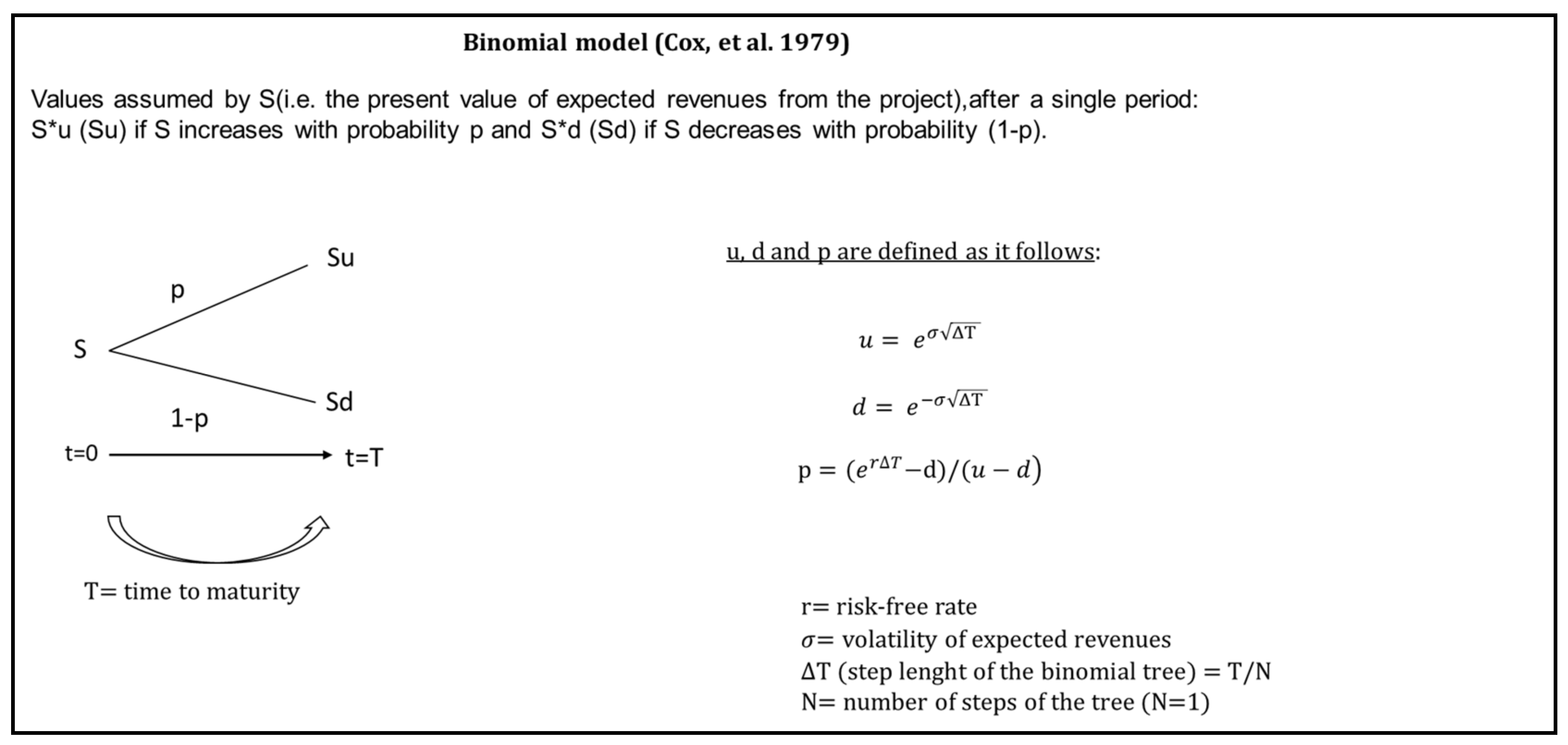
The value of such “wait and see” investment opportunity, or Expanded NPV, is a typical call option, and the version of the option used in this research is analogous to what is found with financial call options. For the purpose of valuing the option to wait and deriving the theoretical benchmark value needed, we use the principles outlined in the well-known and simple-to-use binomial option pricing model by Cox et al. [29], known to have a good fit with valuing simple real options of the type used in the experiment. For details on the method and how it works, we refer the interested readers to see the seminal article or to consult one of the better known textbooks on finance (e.g., [30]). The model we use is very simple, but suitable for the purposes of studying investment decision-making behavior under uncertainty and in the presence of an option to wait to make the investment-decision. Substantially, what we are looking at is a single period binomial option problem—we consider a simplified decision-making situation, where two possible outcomes for an investment are available: A higher outcome with probability p, and a lower outcome with probability (1 − p) (see Figure 1).
Whether the project will generate a higher or a lower outcome is revealed only after a period of time at time T, and is unknown at the beginning of the experiment, i.e., at time 0 (t0).
The participants are asked to choose between a strategy of making an investment up front and taking their chances with the project, and the strategy of (attempting) to acquire an option (at a cost) and making the decision to invest at T, when the outcome of the project is known The first choice means facing a situation that corresponds to using a passive “net present value logic” (NPV), and is here called the “NPV-strategy”, and the second corresponds to a situation where the decision maker can acquire a real option that allows her to postpone the investment decision until the uncertainty is resolved, and is here called the “RO-strategy”. These two alternative strategies are in the heart of this research, as we investigate which one of them is adopted by the decision makers. For the purposes of this study, we use two investment cases that differ by the time to maturity, and correspondingly by the revealed payoffs from the project, that is, whether the project has a higher or a lower outcome, at the time to maturity. Details of the two cases are discussed in the following two subsections.
2.1. NPV-Strategy, the Two Cases
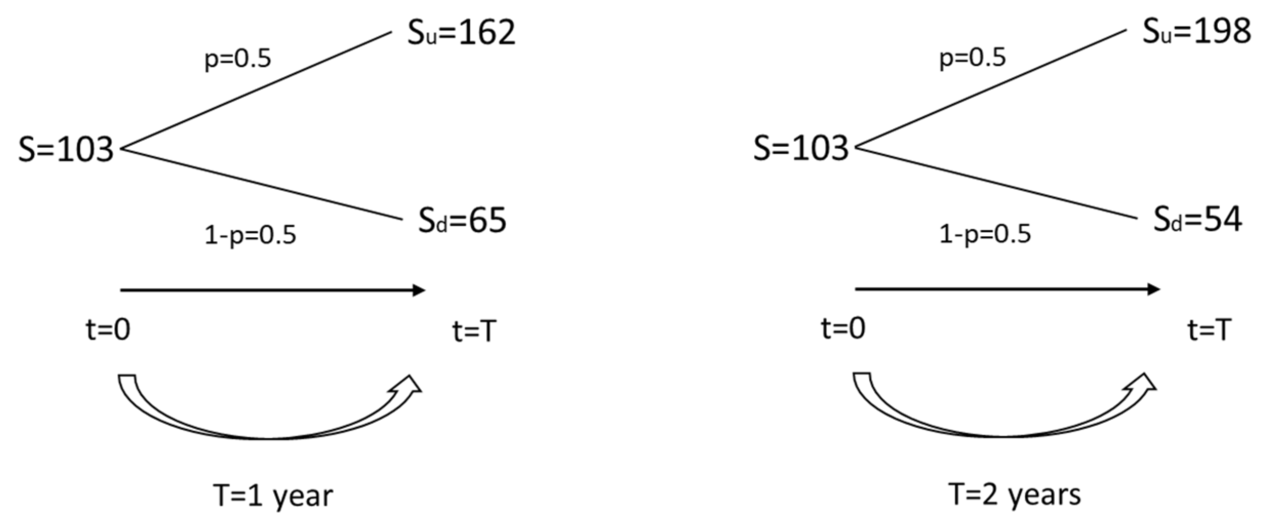
As discussed above, in the NPV-strategy an irreversible investment (I) of 100 experimental currency units (ECU) is made into the project at t0. The outcome of the project is revealed only at time T, during which the pay-off from the project is also clarified. In the first case, the time to maturity is one year (T = 1), and in the second case, two years (T = 2). Moreover, assuming that the risk-free rate (r) is set at 10%, the yearly volatility is assumed to be ~0.46, and the present value of expected revenues (S) is assumed to be 103, two equally probably outcomes may arise: A positive outcome (where the investment is profitable), and a negative outcome (where the investment creates a loss).
Figure 2 shows the positive (Su) and the negative (Sd) outcomes in terms of ECU for both cases, and the expected value of the NPV-strategy (S) at the start of the experiment t0.
The ECU values for the project outcomes have been calculated in line with the standard practice of binomial tree generation illustrated in Figure 1. For the sake of clarity, we note that the numbers used have been rounded for the purposes of the experiment. The expected value of the project at t0 (i.e., the passive NPV which disregards flexibility) is in both cases 103, which makes, in both cases, the net payoff from the project equal to 3 (S − I = 103 − 100 = 3). This means that in both cases, the NPV-strategy has a positive expected NPV, before the uncertainty is resolved, but the decision maker takes a risk and can end up with a loss in the case the project will generate the lower value (Sd).
2.2. RO-Strategy, the Two Cases
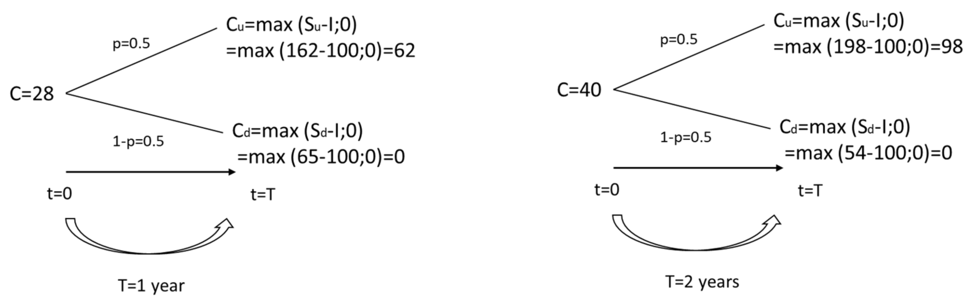
In the RO-strategy, the decision maker postpones the decision-making by acquiring a real option (to postpone). The investment is made at the maturity of the option, time T, only if the outcome of the project is positive, that is, the decision maker will have full knowledge of the outcome at the time, when the decision has to be made—the uncertainty has been resolved. The decision maker will only enter the project if the outcome is the positive one. If the outcome is the negative one, the decision maker will not make an investment into the project. The outcome from the project at time T with the RO-strategy is max In both cases, the decision maker will pay the cost of the option, set at 20 ECU, after time T (see Figure 3).
Again, we account for two cases, where in the first case the time to maturity is one year (T = 1), and in the second case, two years (T = 2). In the first RO-strategy case, by applying the risk-neutral probability measure, the expected value of the project, seen as a call option, at t0 is C = (0.5 × 62 + 0.5 × 0) × e-0.1 = 28. Therefore, the expected payoff from the project, i.e., the expanded NPV including the value of the option to postpone the opportunity to invest in 1 year-time, net of the cost of the option, is 8. This is higher than the expected payoff from the NPV-strategy ceteris paribus (8 > 3). In the second RO-strategy case, respectively, the expected value of the project at t0 is C = (0.5 × 98 + 0.5 × 0) × e-0.1×2 = 40. Therefore, the expected payoff from the project, i.e., the expanded NPV including the value of the option to postpone the opportunity to invest in 2 years-time, net of the cost of the option, is 20. We note that the expected payoff from the RO-strategy in the second case is (considerably) higher than that from the NPV-Strategy in the second case (20 > 3).
The above four cases, two NPV-strategy cases (two passive NPV values) and two RO-strategy cases (two expanded NPV values), are used in the experiments to investigate the decision maker’s behavior.
3. The Experiment
A laboratory experiment was designed and conducted to investigate decision-making behavior in the presence of the flexibility to postpone the investment decision by using the investment problem described above. The experiment consisted of two main stages: In the first stage, subjects performed a real-effort task in order to earn “money” to finance the investment in the second stage. In the second stage, the subjects are obligated to make an investment-decision according to what is explained above.
3.1. Experimental Design and Tasks
Stage 1: Real-Effort Task
Subjects are asked to complete the “slider task” introduced by Gill and Prowse [31] under a fixed pay scheme. The task consists of moving the mouse on a computer to adjust the cursor to a pre-specified position on a slider. Subjects have 10 min to complete as many tasks as they can. They earn 100 ECU for the slider-task. This stage is designed to mandate the subjects to exert effort to earn an endowment for the next stage—the logic is that this task should trigger the participants to perceive the ECU as legitimately earned (asset legitimacy), and not as a sort of wind-fall gift without a true value. Here we depart from the previous experimental studies [21,24], in which the endowment was given to the subjects by the experimenters without inducing any kind of asset legitimacy. Prior research in experimental economics has provided evidence that the origin of the endowment (earned vs. windfall) may influence subject behavior (see, [32]). Most importantly, the design used here is more in line with the real-world situations, where investors make decisions with their earned, not windfall, money.
Stage 2: Investment Decision-Making Under Uncertainty
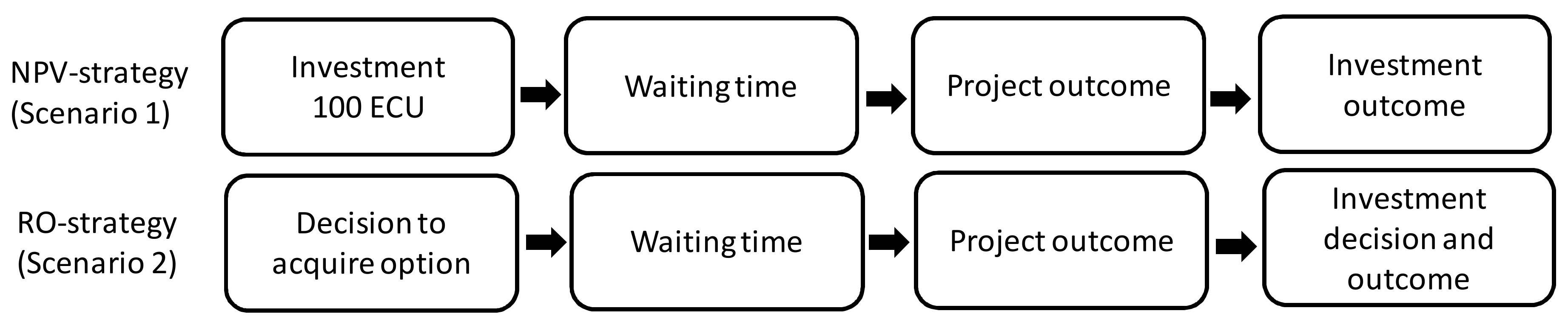
In this stage of the experiment, the subjects have to invest 100 ECU they have earned in Stage 1 into a project with a 50% chance of success. The decision problem is of the type already described above, that is, the choice is between investing with the NPV-strategy immediately and taking the chance between a good and a bad alternative (Scenario 1), and investing with the RO-strategy by committing to pay for an option and having the flexibility to make the investment decision only after the uncertainty about the project outcome has been resolved (Scenario 2). The two scenarios are illustrated in Figure 4.
To be able to invest by using the RO-strategy (Scenario 2) the subjects need to make the decision to acquire the option at a cost. In order to do this, the subjects who want to use the RO-strategy are asked to indicate a cost X from a range between 0 ECU and 30 ECU that they are willing to pay for the option to wait (and for entering Scenario 2). The option has a price Y, which is predetermined and unknown to the subjects. If the X indicated by the subjects is equal or higher than Y, the subjects pay Y for the option and use the RO-strategy. If the indicated X is lower than Y, they do not get the option, and have to invest according to Scenario 1. Here the Y was set at 20 ECU. This technique is a slightly modified version of a famous method used to elicit the reservation prices of consumer goods, originally proposed by Becker et al. [33].
Two experimental treatments are made, where in the first treatment the parameters correspond to the above-described “first case” with the time to maturity of 1 year, and where in the second the parameters correspond to the above-described “second case” with the time to maturity of 2 years. In the first treatment, the laboratory waiting time to mimic the time to maturity of 1 year, was set equal to 20 min—respectively, the laboratory waiting time was set to 60 min for the second treatment (to mimic the 2 years, longer time to maturity).
However, increasing the time to maturity from 1 year to 2 years not only implies that people in the laboratory had more time to wait (from 20 min to 60 min), but it also affects the project outcomes (payoffs). To disentangle the effect of waiting (in real-time) from the effect caused by the different payoffs, we also test for the cases where the call option values corresponding to T = 2 are realized, when the waiting time is 20 min, and where the call option values corresponding to T = 1 are realized, when the waiting time is 60 min. These four choices are called here the “low option value 20/60” and the “high option value 20/60” treatments, respectively. Table 1 shows the details of the four different treatments (see Appendix A for the experimental instructions).
Having the chance to investigate “all” four combinations between the experimental waiting time used and the value parameters, we can disentangle the role played by the “theoretical time” of the model (captured by the option value) and the role played by the experimental “real time”. In fact, the experimental design allows us to investigate two (opposite) situations:
- (a)
- Participants are considered as perfect rational decision makers, which means that they make decisions focalizing exclusively on the consequences generated by the value of the option computed given the theoretical time. Therefore, the participants make decisions based on an evaluation of the investment outcomes, independently from the fact that they are requested to wait 20 min or 60 min in the laboratory.
- (b)
- Participants are considered as decision makers who are psychologically influenced by the length of the real-time they have to spend in the laboratory. Therefore, the participants evaluate differently the utility that they gain from equal investment-outcomes as a consequence of the amount of real time that they spend in the laboratory.
Situation a) indicates a condition in which the participants cognitively "sterilize" the effect of the duration of real-time in the laboratory because the experimental time does not determine the outcome of the investment. On the other hand, situation b) indicates a condition in which the participants psychologically "calibrate" the outcome values, weighing them differently, depending on whether the game is resolved in a short, or in a long real-time.
During the waiting time, participants are presented with two tasks, including the Convex Time Budgets (CTB) task introduced by Andreoni and Sprenger [34] and the Bomb Risk Elicitation task (BRET) introduced by Crosetto and Filippin [35]. In the BRET, participants are given 64 boxes. They are told that, among the boxes, there is one with a bomb, while the other 63 boxes contain 1 ECU each. Participants are asked to collect as many boxes as they want, being informed that in the case the box with the bomb is collected, it would nullify the total amount of ECU earned in this task. The boxes are then opened. If participants do not collect the box containing the bomb, then their earnings increase with the number of accumulated boxes. Conversely, in the case the box with the bomb is collected, participants’ earnings are null. The higher the number of collected boxes, the more risk-taking the participants are. In the CTB task, participants are given an endowment of 80 ECU and 15 budget decisions. In each decision, they are asked to choose their preferred payment between a soon payment date and a delay payment one. The dates and interest rates are different across budget decisions. At the end of the experiment session, one of the participants is randomly chosen, and one of his 12 decisions is randomly selected for payment. The CTB and BRET tasks are used to elicit the subjects’ time and risk preferences, respectively.
If subjects complete the two tasks in less than 20 min/60 min, they watch a nature documentary until the time is up. After the waiting time, subjects are informed about the project outcome and about their final payoffs.
3.2. Participants and Procedures
We ran 8 experimental sessions in October and November 2019 at the Cognitive and Experimental Economics Lab (CEEL) at the University of Trento using the oTree software introduced by Chen et al. [36]. The experiment involved 185 subjects, who are students of the University of Trento and were recruited through an on-line recruitment software. Among the 185 subjects, 60% are economics students and about 44% male—their age ranges from 18 to 31 years old.
Before an experimental session started, subjects were randomly assigned a number which corresponds to their computer position. After they settled down, we delivered to each of them a printed version of the experimental instructions for Stage 1, read instructions out loud, and asked if subjects have any questions. After they completed Stage 1, the same procedures were repeated before Stage 2. Moreover, before subjects made decisions in Stage 2, we gave them 4 control questions about their understanding of the task. Subjects could only proceed further after answering all 4 control questions correctly. During the course of the experiment, subjects could still ask questions at any time by raising their hands. By doing so, their understanding of the experiment is guaranteed.
It is worth underlining that the use of students as experimental subjects is a widely consolidated practice in experimental economics. A number of studies have addressed the question about whether there exists a difference between student and non-student subject pools, and found that the use of students as experimental subjects does not matter much, as the results are much the same (e.g., [37,38,39]).
A between-subject design was implemented, where each subject participated in one treatment only. During the experiment, all the monetary values were expressed in experimental currency units (ECU), and their exchange rate to Euros was 10 ECU = 1 Euro. Subjects were given the exchange rate in advance, and they were privately paid the earnings from their investment into the project resulting from their chosen strategy in cash at the end of each experimental session. Subjects earned, on average, 16.40 euro, including a show-up fee of 3 euro.
4. Predictions Development
The theoretical framework discussed in Section 2 assumes risk neutrality to evaluate the decision to buy or not the right to exercise the option to “wait and invest” after a given time interval. Under such assumption, we have seen that the decision maker should always purchase the opportunity to wait, regardless of the length of the time interval. The ingredients of this decisional dilemma are two: The first is represented by the uncertainty component of the consequences, while the second one is linked to the duration of the time interval that separates the choices from the consequences. Assuming a perfectly rational decision maker, the normative predictions made by the theoretical model are straightforward, because what matters ultimately are only the expected values of the alternative outcomes from the investment, given a discounting factor r, which in the model is assumed to be equal to the risk-free rate. The preferences of the decision maker are trivial: Given risk neutrality, the decision maker always prefers the alternative that ensures the greatest expected discounted outcome, no matter how long she has to wait. These considerations allow us to make the following theory-based hypothesis:
H1T (Theoretical):
If players are risk-neutral and profit maximizing, they should always wait and make the investment decisions at maturity.
This theoretical prediction could change, if we should abandon the standard assumption of perfect rationality for what it regards the role played by time in this decisional setting. In fact, the Behavioral Economics literature has demonstrated that real decision makers almost never behave as the standard inter-temporal decision-making models predict [40]. More precisely, there are more streams of literature that specifically deal with inter-temporal decisions, and among them, at least two are of some relevance for our topic. The first line of literature has shown that the standard exponential inter-temporal discounting model is not able to predict actual choices. The second one has highlighted how decision makers’ anticipated utility may influence their choices.
The failure of the assumption of inter-temporal dynamic consistency implied by the adoption of an exponential discounting function is primarily supported by the empirical evidence that people tend to ask for higher interest rates when the time horizon is short, and for lower interest rates when they cope with a long term time horizon. To model this type of (dynamically inconsistent) inter-temporal preferences, it is correct to use a hyperbolic, or a quasi-hyperbolic discounting function. Quoting Laibson [41] (pp. 445–446):
“Hyperbolic discount functions are characterized by a relatively high discount rate over short horizons and a relatively low discount rate over long horizons. This discount structure sets up a conflict between today’s preferences, and the preferences that will be held in the future. For example, from today’s perspective, the discount rate between two far-off periods, t and t + 1, is the long-term low discount rate. However, from the time t perspective, the discount rate between t and t + 1 is the short-term high discount rate. This type of preference change is reflected in many common experiences.”
This theoretical setting is also supported by many empirical results reported from several Behavioral Economics papers (see [42] for a literature review). More in general, the empirical results reported by this literature show how decision makers often prefer immediate gratification to a delayed one when the choice is very close in time, while they tend to prefer delayed outcomes when they decide over a long-term horizon. This kind of hyperbolic discounting preference applies to a wide array of decisions, including food consumption choices [43,44], choices regarding virtues and vices [42], and choices related to monetary rewards [45]. By trying to extract a general teaching from the literature, it could be concluded that decision makers tend to use different systems of preferences according to whether the consequences of their choices manifest themselves more or less remotely over time.
More precisely, a shorter time horizon induces a higher evaluation of a given outcome than a longer time horizon does. Transferred in our experimental setting, this means that among the participants who have decided to buy the option, the value of the utility attributed to the option in the 20-min treatment is higher than the utility value attributed to the equivalent option in the 60-min treatment. From this line of reasoning, it follows that the decision makers, who have decided to try to buy the option, should pay more for buying the option in the shorter experimental time horizon than in the longer.
The behavioral pattern just described is captured by our first behavioral prediction that applies only to those who prefer the Scenario 2:
H1B (Behavioral):
If the inter-temporal preferences of decision makers are hyperbolic, individuals should be willing to pay a higher price to buy the right to exercise the “wait and see” option when the real time (the laboratory time) is short, compared to the long-time condition, assuming the same value of the option.
It is worth underlining that prediction 1B is exclusively referred to what we have just defined “real time” or “experimental time”. Vice versa, if the decision makers decided according to the "theoretical time" no phenomenon of the type described by prediction 1B should be observed. In fact, the parameters used by the model are calibrated assuming a perfectly rational behavior, and therefore sterilize the psychological impact induced on the choices by intervals of longer or shorter time spent in the laboratory.
Moving now to the second strand of literature already mentioned a few lines above, it is useful to refer to the so-called “savoring” and “dread” effects, originally proposed by Loewenstein and Thaler [46]. This psychological mechanism is well described by the following sentence by Loewenstein and Thaler [46] (p. 190):
“We will use the terms savoring to refer to the positive utility derived from anticipating future pleasant outcomes and dread to refer to the negative contemplation of unpleasant outcomes.”
To better explain the concept of savoring and dread, Loewenstein and Thaler [46] mention the results from an experiment discussed in a previous paper by Loewenstein [47], where the experimental subjects were requested to declare their willingness to pay for delaying or anticipating five positive and five negative outcomes. More precisely, quoting Loewenstein [47] (pp. 667–668), the participants were required to state:
…the ’most you would pay now’ to obtain (avoid) each of five outcomes, immediately, and following five different time delays. The outcomes were: (1) obtain four dollars; (2) avoid losing four dollars; (3) avoid losing one thousand dollars; (4) avoid receiving a (non-lethal) one hundred and ten volt (5) obtain a kiss from the movie star of your choice. Time delays were: (1) immediately (no delay); (2) in twenty-four hours; (3) in three days; year; (4) in one year; (5) in ten years. Subjects were asked to specify the most they would pay for every combination of outcome and time delay.
The main and more interesting results reported by Loewenstein [47] are those referred to the non-pecuniary outcomes (the electric shock and the movie star kiss). The results referred to these two items are counterintuitive if we adopted a standard rationality perspective. In fact, a perfect rational decision maker should be willing to anticipate the positive outcome (the kiss) and to delay the negative one (the shock). On the contrary, the results shown a mirror-like behavior with a sharp tendency of the participants to postpone the kiss and to anticipate the shock. Loewenstein [47] explains this phenomenon by introducing the idea that the decision makers sometime decide by looking their “anticipated utility”. More precisely in the case of the kiss, they prefer to postpone it (obviously not forever) because they are “savoring” the pleasure of being kissed by the movie star, while in the case of the shock, they prefer to anticipate it in order to eliminate the anticipated grief.
Going back to our experimental setting, it is difficult to build a direct relationship between the anticipation of utility and the alternatives that our decision makers were confronting. To buy the option means to go for a safer choice, while to invest immediately means to bet on a riskier but potentially higher outcome. In particular, one could reasonably assume that to wait for the resolution of the uncertain event, implied by the decisional dilemma here designed, would induce some kind of negative utility on the participants due to the psychological feeling of anxiety induced by the fear to incur a loss. This implies that the decision to buy the option is a way to “close the gap” between the present (the time when the decision is taken) and the future, eliminating the anxiety to discover that the investment was a failure. A corollary of this situation is that the longer the delaying, the more “costly” should be perceived the expecting of the potentially negative outcome. This allow us to formulate a second alternative behavioral hypothesis:
H2B (Behavioral):
If the decision makers perceive the risk of an unsuccessful investment as a negative anticipated utility, they should be more likely to buy the right to exercise the option (Scenario 2) when the experimental time is longer compared to the short time condition.
It is worth noticing that the H2B is conflicting with the preceding H1B. This does not mean that only one or the other of the two psychological mechanisms that support these hypotheses is at work, while the other is completely absent. More realistically, it can be said that in the observed behaviors, one or the other of the two cognitive/psychological processes prevails over the other.
5. Results
We first examine whether subjects made decisions consistent with the normative solution of our theoretical model. Assuming decision makers to be risk-neutral profit maximizers, they should always choose Scenario 2, that is, they should always wait and make decisions at maturity. It should be noted that before subjects stated their willingness to pay to obtain the right to exercise the option, they are asked which Scenario they would choose. Those who immediately chose Scenario 1 are not asked about their willingness to pay for the option, whereas those who chose Scenario 2 are asked. Hence, in our setting, there are three types of decision makers:
- Type 1—are those who did not want to benefit from flexibility and always chose Scenario 1;
- Type 2—are those who wanted to buy the right to exercise the real option, but were not willing to pay enough to buy it;
- Type 3—are those who successfully obtained the right to exercise the option.
Table 2 tabulates the proportion of types across treatments.
As Table 2 shows, 39.5% of the participants behave fully in accordance with the RO logic (the Type 3 participants). Meanwhile, the same number tried to enter in Scenario 2, but made an offer to buy the real option, which was below the rational offer (Type 2 participants). Therefore, our experimental results show that a non-negligible percentage of participants violates the predictions of the theoretical model. Moreover, about 21.1% of subjects (Type 1) chose directly Scenario 1. This evidence leads us to the first result.
Result 1:
Overall, nearly 60% of subjects did not enter in Scenario 2, thus revealing a behavior that departs from fully rational decision-making. Among these, more than 20% of subjects do not recognize any benefit from the adoption of the real option logic.
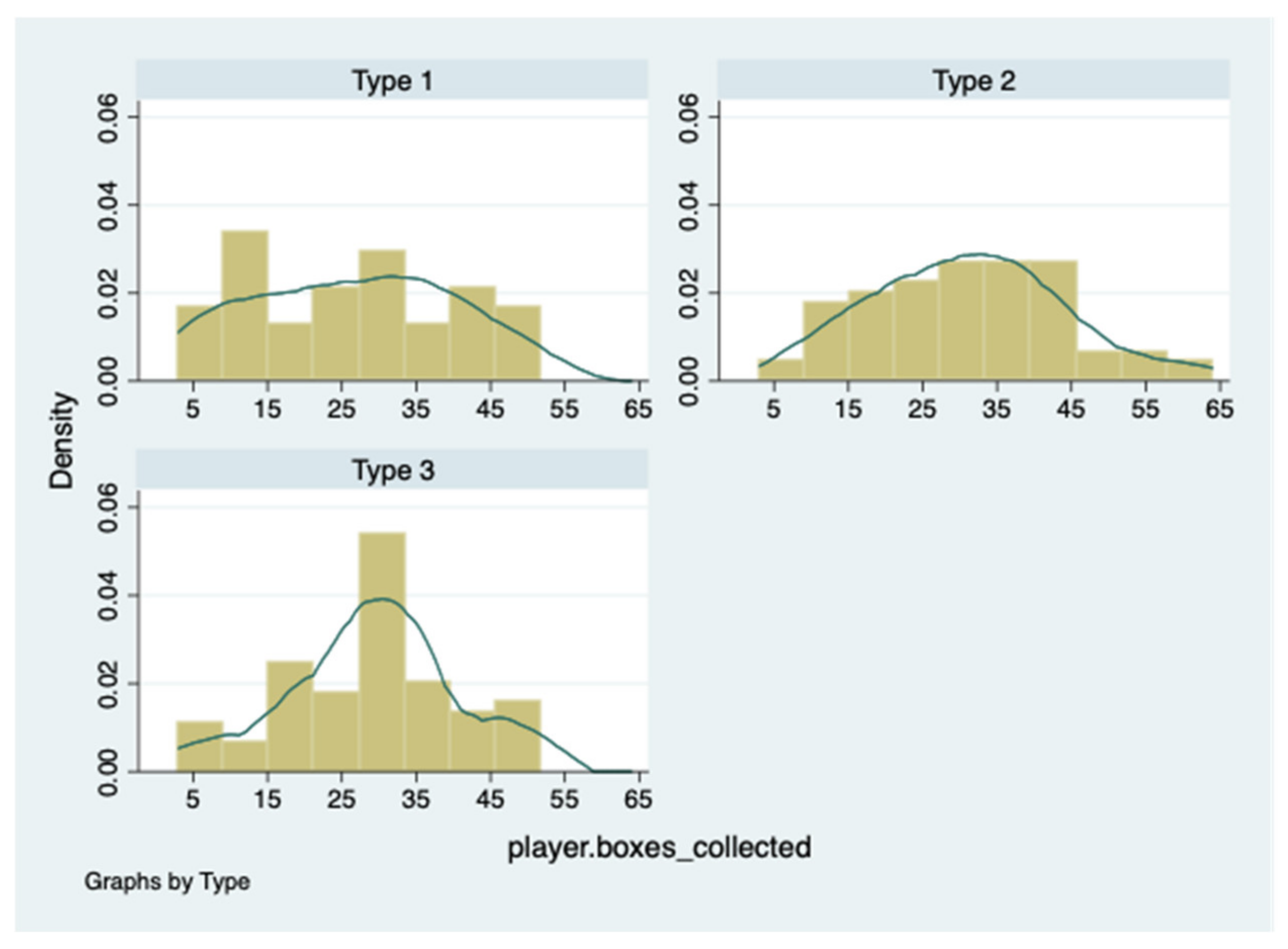
It is important to underline that this result is not affected by the risk attitudes of the participants that are uniformly distributed across the types. Figure 5 illustrates the distribution of number of collected boxes in BRET across types. On average, Type 1, Type 2, and Type 3 collected, respectively, 26, 31, and 29 boxes.
Using the Mann–Whitney test, we do not find any significant differences in risk attitudes across subject types. The results of the test in terms of p-values are presented in Table 3.
To investigate the effect induced by the experimental parameters (that in turn influence the project outcomes) regardless of the real laboratory waiting time, we compare choices in the low option value 20 and low option value 60 treatments with the choices made in the high option value 20 and high option value 60 treatments. Specifically, we compare the number of Type 3 participants in the low option value treatments (26 out of 89) with the number of the same Type in the high option value treatments (47 out of 96). We notice that when the experimental parameters are calibrated on the theoretical 2-year time (high option value), a significantly higher number of subjects is willing to enter into the Scenario 2 and make an offer accordingly with the theoretical model (two-sided Fisher’s exact test, p = 0.007). We summarize these results as follows:
Result 2:
Overall, subjects are more prone to adopt the real options logic when the experimental parameters are calibrated on a theoretical longer time to maturity (2 years), that is, when the value of the option is higher.
This result seems to show that the participants do focalize on the theoretical properties of the decisional dilemma when the parameters are calibrated on a longer theoretical time interval instead of focalizing on the duration of the laboratory real-time. That is, when the option value is higher. This also allows us to say that the participants behave according to a perfect rationality assumption, regardless of the time they have to spend in the laboratory, only when the value of the option is higher. Hence our H1T is only partially supported.
We now look at the effect induced by the laboratory real-time regardless of the option value, (that is 20 min, or 60 min), thus comparing choices in the low option value 20 and high option value 20 treatments with choices in low option value 60 and high option value 60 treatment. Specifically, we compare the number of Type 3 participants in the 20-minute treatments (43 out of 92) with the number of the same Type in the 60-minute treatments (30 out of 93). We notice that participants behave more in accordance with the theoretical model when the laboratory real-time is shorter (20 min). Indeed, in such a case, the percentage of subjects of Type 3 is significantly higher than it is in the longer laboratory real-time condition (two-sided Fisher’s exact test, p = 0.051). In the laboratory real short time, compared to the laboratory real long time, subjects are more prone to avoid uncertainty. That is, the psychological cost of waiting is lower in the actual short time rather than in the actual long time.
Result 3:
Overall, participants are more prone to adopt the real option logic when the laboratory real time is shorter.
Next, we investigate on the effect induced by the option values when the laboratory real time is either short or long. Thus, we compare choices between the low option value 20 and the high option value 20 treatments, as well as the choices between low option value 60 and high option value 60 treatments. We observe that in the high option value 60 treatment, there is a significantly higher number of subjects of Type 3 than in the low option value 60 treatment (two-sided Fisher’s exact test, p = 0.016). However, there is no such a difference between the low option value 20 treatment and the high option value 20 treatment. These findings suggest that only when making decisions in a longer laboratory real time, the value of the option represents a crucial factor on subjects’ investment decisions.
Result 4:
The value of the option (i.e., the value of the option calibrated on 1- year time or 2-year time) has an effect only when the laboratory real time is long (i.e., 60 min): When the value of option is high (i.e., when the option values are calibrated on 2-year time), subjects are more prone to adopt a real option logic. Conversely, the value of the option has no effect when the laboratory real time is short.
Moreover, we investigate on the effect induced by the laboratory real time when the option values are either calibrated on a 1-year time or a 2-year time. Thus, we compare choices between the low option value 20 and low option value 60 treatments, as well as choices between high option value 20 and high option value 60 treatments. We observe that, in the low option value 20 treatment, there is a significantly higher number of subjects of Type 3 than in the low option value 60 treatment (two-sided Fisher’s exact test, p = 0.065). However, there is no such difference between the high option value 20 treatment and high option value 60 treatment. These findings suggest that only when the option values are calibrated on a 1-year time, the waiting laboratory real-time represents a crucial factor on subjects’ investment decisions. This allows us to summarize as follows:
Result 5:
The laboratory real-time has an effect only when the value of the option is low (i.e., when the option value is calibrated on a 1-year time): When the laboratory real-time is short, subjects are more prone to adopt the real option logic. Conversely, the laboratory real-time has no effect, when the value of the option increases (i.e., when the option value is calibrated on 2-year time).
Lastly, we shed light on the subjects’ Willingness To Pay (WTP) for the option to wait to make the investment decision. On average, subjects in the different treatments were willing to pay 20.3 ECU (low option value 20), 19.8 ECU (high option value 20), 17.5 ECU (low option value 60) and 21.2 ECU (high option value 60). The distribution of subjects’ willingness to pay across treatments is depicted in Figure 6.
Table 4 tabulates the Tobit-regression result of WTP on treatments, subjects’ risk (captured by the variable BRET) and time preferences (captured by the variable “delta_ind”), as well as demographic characteristics including gender, age, and the field of study. We found the treatment effect only between the low option value 20 and the low option value 60 treatment. This result confirms the findings summarized in Result 5: The real-laboratory waiting time plays an important role only when the option value is lower.
Result 6:
When the value of the option is low (i.e., when the option values are calibrated on 1-year time), subjects are more willing to pay for acquiring the right to exercise the real options when the laboratory real time is shorter.
It follows that our first behavioral Hypothesis is only partially supported (i.e., only when the option value is low) while our second behavioral hypothesis is not confirmed.
By means of Mann–Whitney tests, we find that the WTPs are significantly higher in the treatment with long real experimental time and high option value (high option value 60) than in the treatment again with long real experimental time but with low option value (low option value 60) (Mann–Whitney test, p = 0.025). Additionally, we confirm that the WTP in the treatment with low option value and short experimental time (low option value 20) is significantly higher than the WTP in the treatment with low option value and high experimental time (low option value 60) (Mann–Whitney test, p = 0.049).
6. Conclusions
Our study focuses on examining the investment decision-making process at the individual level. We join the emerging and promising stream of studies that utilize experimental laboratory designs to closely investigate decision-making behavior in a real options based mechanism [12,13,14,15,16,17]. By doing so, we contribute to the managerial literature regarding micro-foundations of investment decision-making under uncertainty.
Despite several real options theory-based contributions having been developed and have helped decision-makers cope with uncertainty in theoretical terms, they have ignored important aspects of the behavioral environments in which investment decisions take place [20]. Our research is in line with experimental studies on real options (e.g., [20]) that offer support for applying recent findings from behavioral research to comprehend how individuals really think about real options.
Specifically, we designed an experiment that presents two fundamental features of the classical real options approach. First, decision makers have to make an irreversible investment. They can choose between a risky decision (i.e., to invest immediately, accepting the risk to waste the investment) and a safe alternative (i.e., wait and invest only if conditions are favorable). Second, the benefit of waiting is emphasized: It is optimal for decision makers to delay and keep the option alive until the uncertainty is solved. We find that, regardless of the laboratory waiting time, decision makers recognize the benefit of waiting only when the value of the option is higher, i.e., when the experimental parameters are calibrated on a theoretically longer time to maturity (2 years). On the other hand, when the option assumes a lower value (i.e., when the option values are calibrated on a 1-year time), subjects are more willing to pay for acquiring the right to exercise the real option, when the laboratory waiting time is shorter.
Our results provide interesting implications for policy makers because they demonstrate that people make different decisions based on whether they pay more or less attention respectively on the value of the option or on the duration of the laboratory time required to solve uncertainty. The tendency to focalize more intensely on the value of the option, neglecting the temporal component of the decisional dilemma, typically happens when the option value is high. Conversely, when the value of the option is low, the decision makers tend to address their attention more on the time needed to solve uncertainty. As a consequence, people make decisions that are different from those that they would make if they were perfect rational agents. Actually, perfect rationality implies that the decision makers are not influenced by any kind of distortions induced by the decisional context (framing). This also means that if the decision makers were managers, one must be aware of the risk that they could assume in an “irrational” way the decisions regarding this kind of financial tools (real options). In fact, from the results of our experiments, we know that both the values attributed by the participants to the option and to the time needed to solve uncertainty are a matter of subjective “perception”. Hence, they cannot be considered like an objective, inter-personally constant and equal dimension of the choice problem. These findings suggest to build the company strategy towards a direction which is different from the theoretical normative optimal, and more importantly, more sustainable path.
Our results are in line with earlier findings on the ability of experiment participants not being able to fully rationally price the flexibility brought by options [20], and in line with previously recorded behavior with regards to inter-temporal decision-making [21].
A number of further directions can be taken to build upon this work. First, in order to better understand the role of the theoretical time to maturity which influences the value of the option as well as of the laboratory waiting time, future laboratory studies could employ investment scenarios where different theoretical and laboratory times are implemented. Second, in this study, we focused, both theoretically and experimentally, on call options where subjects need to decide whether to acquire the right to postpone an investment opportunity. It would be interesting to extend such analysis in the domain of put options where subjects must decide whether to acquire the right to abandon an investment opportunity.
Another interesting setting would be introducing strategic interactions. In fact, the introduction of competition may change the optimal investment timing theoretically. For instance, in the case subjects compete for buying the option, instead of waiting, anticipating the time of acquiring the right to exercise such an option may be more convenient. It would be useful to experimentally test this particular setting and to investigate on the role of both the theoretical time to maturity, and of the laboratory waiting time in such a situation. Finally, further studies with field experiments on different target populations, such as real-world investors, MBA students, and managers, would be necessary to enhance the external validity of our results.
Author Contributions
Conceptualization, A.M. and L.M.; formal analysis, A.M. and T.-T.-T.V.; investigation, A.M., L.M. and T.-T.-T.V.; methodology, A.M. and L.M.; software, T.-T.-T.V.; visualization, A.M., L.M., T.-T.-T.V. and M.C.; writing – original draft, A.M., L.M., T.-T.-T.V.; writing – review & editing, A.M., L.M., T.-T.-T.V. and M.C.; supervision, L.M.; funding acquisition, A.M., L.M. and M.C. All authors have read and agreed to the published version of the manuscript.
Funding
This research was supported by Arvopaperimarkkinoiden Edistämissäätiö research grant.
Acknowledgments
The authors would like to thank Marco Tecilla for programming the experimental software.
Conflicts of Interest
The authors declare no conflict of interest.
Appendix A.
Experimental instructions of the two 20-minute treatments (parameters of the “high option value 20” treatment are in brackets) are translated from Italian. Instructions of the 60-minute treatments only differ in the waiting time.
Welcome! This is a study of economic decision making. The study includes three tasks and a questionnaire. After completing a task, you will participate in the next task and earn more money. All tasks will be computerized. In each task, all participants will receive the same instruction. In all instructions, we will always provide you true information that never deceives you in any way.
The choices made by each participant will be confidential unless explicitly specified. Anonymity will be maintained both during and after the study: Your identity will not be made known to any participant at any time.
You will have the opportunity to earn tokens in each of the three tasks. The tokens you earn in each task cumulate and will be converted into Euro at the end, at the rate of 1 Euro for every 10 tokens. You will also receive 3 euros for showing up in this study. The money you earn will be paid to you in private, and in cash, at the end of the study.
We ask you to turn off your phone now and not to communicate in any way with the people present in the room until the end of the study. If you have any questions, please raise your hand and we will assist you in private. You are free to leave the study if you want to, however, you will not receive any sum of money.
- 1. Task 1
Your task is to adjust each slider from the initial position 0 to the desired position by pressing the cursor with your mouse and dragging it. When you drag the cursor, the number on the right will tell you the current position of the cursor. The cursor is positioned correctly when the current position equals the “target” number. By clicking “Next”, you will be presented new sliders to adjust.
You have 10 min and will earn 100 tokens in this task.
- 2. Task 2
In this task, you have to make an investment decision with the 100 tokens you earned in Task 1.
You can choose two Scenarios.
Scenario 1
In this Scenario, you invest immediately 100 tokens. Your investment outcome will depend on the result of lottery: With 50%, the lottery outcome is 162 [198] tokens, and with 50%, the lottery outcome is 65 [54] tokens. It means that you will earn 162 [198] tokens with probability 0.5, and 65 [54] tokens with probability 0.5. It should be noted that by choosing this Scenario, you will invest your 100 tokens before knowing the lottery outcome. You have to wait 20 min to know the lottery outcome. In other words, in Scenario 1, you invest immediately 100 tokens and after 20 min, you will have a 50% chance getting 162 [198] tokens or 65 [54] tokens. The table below summarizes your payoff possibilities in Scenario 1:

Table A1.
Summary of payoff possibilities in Scenario 1.
| Investment | Wait 20 min | Lottery Outcome | Final Payoffs |
|---|---|---|---|
| 100 tokens | YES | 162 [198] tokens with 50% | 162 [198] tokens |
| 100 tokens | YES | 65 [54] tokens with 50% | 65 [54] tokens |
Scenario 2
In this Scenario, you invest 100 tokens after you already know the lottery outcome. It means that you will also wait for 20 min to know the lottery outcome and make an investment decision. Like in Scenario 1, the result of the lottery is that with 50%, the lottery outcome is 162 [198] tokens, and with 50%, the lottery outcome is 65 [54] tokens. However, your payoff will be different: If the lottery outcome is 162 [198] tokens, you will earn 198 tokens, but if the lottery outcome is 65 [54 tokens, you can get back your 100 tokens.
To access this Scenario, you have to pay some tokens. You have to state the number of tokens from 0 to 30 which you want to pay to access this Scenario. There is already a predefined price to get Scenario 2 called X, which is a number from 0 to 30. If the number you state, called Y, is bigger than or equal to the predefined price X, or Y > X, or Y = X, you will pay X tokens to access Scenario 2. If the number you state Y is smaller than the predefined price X, or Y < X, you will not access Scenario 2 and automatically access Scenario 1. It should be noted that you have to state Y before you know X. The table below summarize your payoff possibilities in Scenario 2:
Table A2.
Summary of payoff possibilities in Scenario 2.
| Wait 20 min | Lottery Outcome | Investment | Final Payoffs |
|---|---|---|---|
| YES | 162 [198] tokens | 100 UMS | (162 − X) [(198 − X)] tokens |
| YES | 65 [54] tokens | No investment | (100 − X) tokens |
References
- Smit, H.T.J.; Trigeorgis, L. Strategic Options and Games in Analysing Dynamic Technology Investments. Long Range Plann. 2007. [Google Scholar] [CrossRef]
- Cassimon, D.; De Backer, M.; Engelen, P.J.; Van Wouwe, M.; Yordanov, V. Incorporating technical risk in compound real option models to value a pharmaceutical R&D licensing opportunity. Res. Policy 2011. [Google Scholar] [CrossRef]
- Savolainen, J. Real options in metal mining project valuation: Review of literature. Resour. Policy 2016. [Google Scholar] [CrossRef]
- Kozlova, M. Real option valuation in renewable energy literature: Research focus, trends and design. Renew. Sustain. Energy Rev. 2017. [Google Scholar] [CrossRef]
- Collan, M. Thoughts about selected models for the valuation of real options. Acta Univ. Palacki. Olomuc. Fac. Rerum Nat. Math. 2011, 50, 5–12. [Google Scholar]
- Collan, M.; Haahtela, T.; Kyläheiko, K. On the usability of real option valuation model types under different types of uncertainty. Int. J. Bus. Innov. Res. 2016. [Google Scholar] [CrossRef]
- Borison, A. Real Options Analysis: Where Are the Emperor’s Clothes? J. Appl. Corp. Financ. 2005, 17, 17–31. [Google Scholar] [CrossRef]
- Hartmann, M.; Hassan, A. Application of real options analysis for pharmaceutical R&D project valuation-Empirical results from a survey. Res. Policy 2006. [Google Scholar] [CrossRef]
- Posen, H.E.; Leiblein, M.J.; Chen, J.S. Toward a behavioral theory of real options: Noisy signals, bias, and learning. Strateg. Manag. J. 2018. [Google Scholar] [CrossRef]
- Thaler, R.H.; Mullainathan, S. How Behavioral Economics Differs from Traditional Economics. Available online: https://www.econlib.org/library/Enc/BehavioralEconomics.html (accessed on 21 February 2020).
- Trigeorgis, L. Real Options Theory under Bounded Rationality; Kings College: London, UK, 2014. [Google Scholar]
- Ma, G.; Du, Q.; Wang, K. A concession period and price determination model for PPP projects: Based on real options and risk allocation. Sustainability 2018, 10, 706. [Google Scholar] [CrossRef] [Green Version]
- Shi, J.; Duan, K.; Wen, S.; Zhang, R. Investment valuation model of public rental housing PPP project for private sector: A real option perspective. Sustainability 2019, 11, 1857. [Google Scholar] [CrossRef] [Green Version]
- Lomoro, A.; Mossa, G.; Pellegrino, R.; Ranieri, L. Optimizing risk allocation in public-private partnership projects by project finance contracts. the case of put-or-pay contract for stranded posidonia disposal in the municipality of bari. Sustainability 2020, 12, 806. [Google Scholar] [CrossRef] [Green Version]
- Kim, S.; Giachetti, R.; Park, S. Real options analysis for acquisition of new technology: A case study of Korea K2 Tank’s Powerpack. Sustainability 2018, 10, 3866. [Google Scholar] [CrossRef] [Green Version]
- Park, J.H.; Shin, K. R & D project valuation considering changes of economic environment: A case of a pharmaceutical R & D project. Sustainability 2018, 10, 993. [Google Scholar] [CrossRef] [Green Version]
- Durica, M.; Guttenova, D.; Pinda, L.; Svabova, L. Sustainable value of investment in real estate: Real options approach. Sustainability 2018, 10, 4665. [Google Scholar] [CrossRef] [Green Version]
- Ranieri, L.; Mossa, G.; Pellegrino, R.; Digiesi, S. Energy recovery from the organic fraction of municipal solid waste: A real options-based facility assessment. Sustainability 2018, 10, 368. [Google Scholar] [CrossRef] [Green Version]
- Dai, H.; Sun, T.; Guo, W. Brownfield redevelopment evaluation based on fuzzy real options. Sustainability 2016, 8, 170. [Google Scholar] [CrossRef] [Green Version]
- Miller, K.D.; Shapira, Z. An empirical test of heuristics and biases affecting real option valuation. Strateg. Manag. J. 2004. [Google Scholar] [CrossRef] [Green Version]
- Yavas, A.; Sirmans, C.F. Real options: Experimental evidence. J. Real Estate Financ. Econ. 2005. [Google Scholar] [CrossRef]
- Oprea, R.; Friedman, D.; Anderson, S.T. Learning to wait: A laboratory investigation. Rev. Econ. Stud. 2009. [Google Scholar] [CrossRef]
- Andersion, S.T.; Friedman, D.; Oprea, R. Preemption games: Theory and experiment. Am. Econ. Rev. 2010, 100, 1778–1803. [Google Scholar] [CrossRef] [Green Version]
- Murphy, R.O.; Andraszewicz, S.; Knaus, S.D. Real options in the laboratory: An experimental study of sequential investment decisions. J. Behav. Exp. Financ. 2016. [Google Scholar] [CrossRef]
- Morreale, A.; Mittone, L.; Lo Nigro, G. Risky choices in strategic environments: An experimental investigation of a real options game. Eur. J. Oper. Res. 2019. [Google Scholar] [CrossRef] [Green Version]
- Amram, M.; Kulatilaka, N. Real options: Managing strategic investment in an uncertain worldChapter 1: Introduction. Harvard Bus. Sch. Press Bost. 1999. [Google Scholar]
- Brach, M. Real Options in Practice; John Wiley & Sons: Hoboken, NJ, USA, 2003. [Google Scholar]
- Smit, H.T.J.; Trigeorgis, L. Strategic Investment: Real Options and Games; Princeton University Express: Princeton, NJ, USA, 2012. [Google Scholar]
- Cox, J.C.; Ross, S.A.; Rubinstein, M. Option pricing: A simplified approach. J. Financ. Econ. 1979. [Google Scholar] [CrossRef]
- Brealey, R.A.; Myers, S.C. Principles of Corporate Finance; Mc-Graw-Hill Companies: New York, NY, USA, 1996. [Google Scholar]
- Gill, D.; Prowse, V. Measuring costly effort using the slider task. J. Behav. Exp. Financ. 2019. [Google Scholar] [CrossRef] [Green Version]
- Carlsson, F.; He, H.; Martinsson, P. Easy come, easy go: The role of windfall money in lab and field experiments. Exp. Econ. 2013. [Google Scholar] [CrossRef]
- Becker, G.M.; DeGroot, M.H.; Marschak, J. Measuring utility by a single-response sequential method. Behav. Sci. 1964. [Google Scholar] [CrossRef]
- Andreoni, J.; Sprenger, C. Estimating time preferences from convex budgets. Am. Econ. Rev. 2012. [Google Scholar] [CrossRef] [Green Version]
- Crosetto, P.; Filippin, A. The ‘bomb’ risk elicitation task. J. Risk Uncertain. 2013. [Google Scholar] [CrossRef] [Green Version]
- Chen, D.L.; Schonger, M.; Wickens, C. oTree-An open-source platform for laboratory, online, and field experiments. J. Behav. Exp. Financ. 2016. [Google Scholar] [CrossRef]
- Depositario, D.P.T.; Nayga, R.M.; Wu, X.; Laude, T.P. Should students be used as subjects in experimental auctions? Econ. Lett. 2009. [Google Scholar] [CrossRef]
- Exadaktylos, F.; Espín, A.M.; Brañas-Garza, P. Experimental subjects are not different. Sci. Rep. 2013. [Google Scholar] [CrossRef] [PubMed]
- Fréchette, G.R. Laboratory Experiments: Professionals Versus Students. In Handbook of Experimental Economic Methodology; Oxford University Press: Oxford, UK, 2015. [Google Scholar] [CrossRef]
- Fisher, I. The Theory of Interest; Macmillan: New York, NY, USA, 1930. [Google Scholar]
- Laibson, D. Golden Eggs and Hyperbolic Discounting on JSTOR. Q. J. Econ. 1997, 112, 443–477. [Google Scholar] [CrossRef] [Green Version]
- Read, D.; Loewenstein, G.; Kalyanaraman, S. Mixing virtue and vice: Combining the immediacy effect and the diversification heuristic. J. Behav. Decis. Mak. 1999. [Google Scholar] [CrossRef]
- Simonson, I. The Effect of Purchase Quantity and Timing on Variety-Seeking Behavior. J. Mark. Res. 1990. [Google Scholar] [CrossRef]
- Read, D.; Van Leeuwen, B. Predicting Hunger: The Effects of Appetite and Delay on Choice. Organ. Behav. Hum. Decis. Process. 1998. [Google Scholar] [CrossRef] [Green Version]
- Thaler, R. Some empirical evidence on dynamic inconsistency. Econ. Lett. 1981. [Google Scholar] [CrossRef]
- Loewenstein, G.; Thaler, R. Anomalies: Intertemporal Choice. J. Econ. Perspect. 1989, 3, 181–193. [Google Scholar] [CrossRef] [Green Version]
- Loewenstein, G. Anticipation and the Valuation of Delayed Consumption. Econ. J. 1987. [Google Scholar] [CrossRef] [Green Version]
Figure 1.
Binomial distribution of project revenues.

Figure 2.
Net present value (NPV)-strategy, both cases, with T = 1 (left) and with T = 2 (right).

Figure 3.
Real options (RO)-strategy, both cases, with T = 1 (left) and with T = 2 (right).

Figure 4.
Stylized illustration of the two alternative investment scenarios.

Figure 5.
The distribution of collected boxes across subject types.

Figure 6.
The distribution of willingness to pay across treatments.

Table 1.
Description of the treatments.
| Treatment | Waiting Time (min) | Project Outcomes | Net Expected Payoff | |
|---|---|---|---|---|
| NPV-Strategy Passive NPV (Scenario 1) | RO-Strategy Expanded NPV (Net of the Cost of the Option) (Scenario 2) | |||
| Low option value 20 | 20 | 162 / 65 (p = 50%) | 3 | 8 |
| High option value 20 | 20 | 198 / 54 (p = 50%) | 3 | 20 |
| Low option value 60 | 60 | 162 / 65 (p = 50%) | 3 | 8 |
| High option value 60 | 60 | 198 / 54 (p = 50%) | 3 | 20 |
Table 2.
Proportion of types across treatments.
| Treatment | Type 1 | Type 2 | Type 3 | Total |
|---|---|---|---|---|
| Low option value 20 | 12 (27.3%) | 15 (34.1%) | 17 (38.7%) | 44 (100%) |
| High option value 20 | 6 (12.5%) | 16 (33.3%) | 26 (54.2%) | 48 (100%) |
| High option value 60 | 10 (20.8%) | 17 (35.4%) | 21 (43.8%) | 48 (100%) |
| Low option value 60 | 11 (24.4%) | 25 (55.6%) | 9 (20%) | 45 (100%) |
| All | 39 (21.1%) | 73 (39.5%) | 73 (39.5%) | 185 (100%) |
Table 3.
Two-tailed p-values from Mann–Whitney test on risk preferences across types.
| Comparison | Mann–Whitney Test (p-Values) |
|---|---|
| Type 1 vs. Type 2 | 0.16 |
| Type 2 vs. Type 3 | 0.49 |
| Type 1 vs. Type 3 | 0.26 |
Table 4.
Tobit regression of Willingness To Pay (WTP).
| Dependent Variable: WTP | Coef | SE |
|---|---|---|
| low option value 20 | Reference | |
| high option value 20 | −0.83 | 1.98 |
| high option value 60 | 0.56 | 2.10 |
| low option value 60 | −3.60 * | 2.09 |
| BRET | 0.01 | 0.06 |
| Male | −0.15 | 1.41 |
| Age | 0.04 | 0.32 |
| Economics | 1.84 | 1.63 |
| delta_ind | −0.00 | 0.00 |
| sigma | 8.05 *** | 0.55 |
| Constant | 18.98 ** | 7.79 |
| Observations | 146 |
Note: *** p < 0.01, ** p < 0.05, * p < 0.1.
© 2020 by the authors. Licensee MDPI, Basel, Switzerland. This article is an open access article distributed under the terms and conditions of the Creative Commons Attribution (CC BY) license (http://creativecommons.org/licenses/by/4.0/).
Share and Cite
MDPI and ACS Style
Morreale, A.; Mittone, L.; Vu, T.-T.-T.; Collan, M. To Wait or Not to Wait? Use of the Flexibility to Postpone Investment Decisions in Theory and in Practice. Sustainability 2020, 12, 3451. https://doi.org/10.3390/su12083451
AMA Style
Morreale A, Mittone L, Vu T-T-T, Collan M. To Wait or Not to Wait? Use of the Flexibility to Postpone Investment Decisions in Theory and in Practice. Sustainability. 2020; 12(8):3451. https://doi.org/10.3390/su12083451
Chicago/Turabian StyleMorreale, Azzurra, Luigi Mittone, Thi-Thanh-Tam Vu, and Mikael Collan. 2020. "To Wait or Not to Wait? Use of the Flexibility to Postpone Investment Decisions in Theory and in Practice" Sustainability 12, no. 8: 3451. https://doi.org/10.3390/su12083451
Note that from the first issue of 2016, this journal uses article numbers instead of page numbers. See further details here.