Comparison of Cloud Cover Detection Algorithms on Sentinel–2 Images of the Amazon Tropical Forest

Abstract

Tropical forests regulate the global water and carbon cycles and also host most of the world’s biodiversity. Despite their importance, they are hard to survey due to their location, extent, and particularly, their cloud coverage. Clouds hinder the spatial and radiometric correction of satellite imagery and also diminishing the useful area on each image, making it difficult to monitor land change. For this reason, our purpose is to identify the cloud detection algorithm best suited for the Amazon rainforest on Sentinel–2 images. To achieve this, we tested four cloud detection algorithms on Sentinel–2 images spread in five areas of the Amazonia. Using more than eight thousand validation points, we compared four cloud detection methods: Fmask 4, MAJA, Sen2Cor, and s2cloudless. Our results point out that FMask 4 has the best overall accuracy on images of the Amazon region (90%), followed by Sen2Cor’s (79%), MAJA (69%), and S2cloudless (52%). We note the choice of method depends on the intended use. Since MAJA reduces the number of false positives by design, users that aim to improve the producer’s accuracy should consider its use.

1. Introduction

The world’s tropical forests are essential places for environmental sustainability and the future of our planet. They combine high biodiversity and significant carbon storage with ecological services [1,2]. Since the 1980s, the world’s tropical forests have undergone substantial change. Agricultural expansion worldwide happened at the expense of tropical forest areas [3]. In particular, the Brazilian Amazon rain forest has suffered significant deforestation. According to Brazil’s National Institute for Space Research (INPE), deforestation has reached 20% of the Amazon rain forest in the country [4]. Producing qualified assessments of land-use and land cover change in Amazonia is essential for evidence-based policies that can protect the forest [5,6].

Earth observation data is the primary source of assessments of deforestation in Amazonia. Since the late 1980s, INPE produces annual estimates of clear-cut areas of forest with the PRODES project and daily indications of deforestation alerts with the DETER initiative [7]. PRODES and DETER are the authoritative sources of information that support Brazil’s actions in protecting Amazonia [8,9]. As a companion to the monitoring of clear-cut areas, INPE and its partners also produce periodic maps of land-use change in deforested areas in Amazonia with the TerraClass project [10]. Universities and research groups complement INPE’s work [11,12]. Altogether, there is a substantial amount of land-use change information on the Brazilian Amazonia derived from remote sensing data.

Despite the widespread data availability, the complexity of land-use transitions in Amazonia requires continuous improvements in image classification. Law enforcement actions by the Brazilian federal government managed to reduce deforestation from 2.7 Mha (million hectares) in 2004 to an average of 0.6 Mha between 2009 and 2018. Despite such reduction, deforestation in Amazonia is still at a relatively high level. To understand the complex interplay between crop production, cattle ranching, and land speculation, ever more detailed data is required.

To improve monitoring of the Amazon forest from satellites, researchers are investigating the use of big data analytics [13,14]. Such methods rely on the increase of data provided by the new generation of satellites such as Sentinel–2 [15]. However, to use these large data sets in tropical forest areas, researchers need suitable methods of automated cloud detection in optical imagery.

Traditional alternatives for dealing with cloud cover include combining information from various dates and selecting a “best pixel” for an extended period [16]. These methods lead to the loss of temporal information required to identify crop types [14,17] and pasture management [18,19]. To capture temporal information, many researchers prefer methods that identify cloud-covered pixels and replace them with interpolated estimates [20]. When different satellites are combined to produce a denser time series [21], replacing cloudy pixels by interpolated values becomes feasible. For this reason, automated cloud detection algorithms are a necessary complement to big Earth observation data analytics.

Cloud detection algorithms are an active research field [20,22,23,24,25]. Each algorithm has specific characteristics and ad hoc techniques; thus, comparing them on a theoretical basis is hard. In practice, performance assessment is done by selecting representative images and assessing how well each algorithm performs in each image. As an example, Baetens et al. [26] compared three cloud detection methods (MAJA, Sen2Cor, and Fmask) using 32 images from 10 different locations. As a reference for comparison, the authors use a machine learning method to identify clouds for Sentinel–2 images. Given the different land cover, the diversity of sensors, and the advances in detection methods, such comparisons serve as general guidance only.

In this paper, we approach the problem of comparing different cloud detection algorithms from a regional viewpoint. Given the importance of monitoring land change in Amazonia, we consider cloud detection methods for Sentinel-2 MSI images in this region. We consider four cloud detection algorithms: Fmask 4 [25], MAJA [23], Sen2Cor 2.8 [22], and s2cloudless [27]. Cloud formation in Amazonia is distinct from most continental areas [28]. The forest produces its own rain [29]. The rainforest generates the aerosols that make up the cloud condensation nucleus in the region [30]. The probabilities of cloud coverage in satellite imagery depend not only on the month of the year but also on the location inside Amazonia [31]. Cloud types are heterogeneous in the Amazon biome; the southern region of the Amazonia has high aerosol concentration, whereas the northern and northwestern regions have low aerosol concentration and high precipitation [30,32]. These characteristics indicate different processes in cloud formation in subregions of the Amazon biome.

During the wet season, the precipitating clouds in the Amazon basin are either low-level stratus type clouds (up to 2–5 km altitude) or high-level convective systems (more than 6 km altitude) [30]. The different land cover influences the amount and type of clouds. Deep clouds are commonly found over the forest while shallow clouds are frequent over deforested areas [33,34]. Water bodies absorb visible and near-infrared radiation diminishing the reflectivity of the thin clouds above [35]. The high reflectivity of artificial surfaces induces commission errors in cloud detection over urban areas [36]. Such differences pose a challenge for cloud detection algorithms in Amazonia; they need to consider many types of cloud formations and associated shadows. These singular characteristics suggest that it is useful to take images over Amazonia as a study case when comparing cloud detection methods.

The rest of this article is organized as follows. We first introduce the study area and the sample regions. Then we present the cloud detection algorithms and how we configured them. Later we show how the classes resulting from each cloud detection algorithm compares to the others. Finally, we introduce our results and then we discuss some implications of this work.

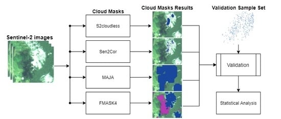
2. Materials and Methods

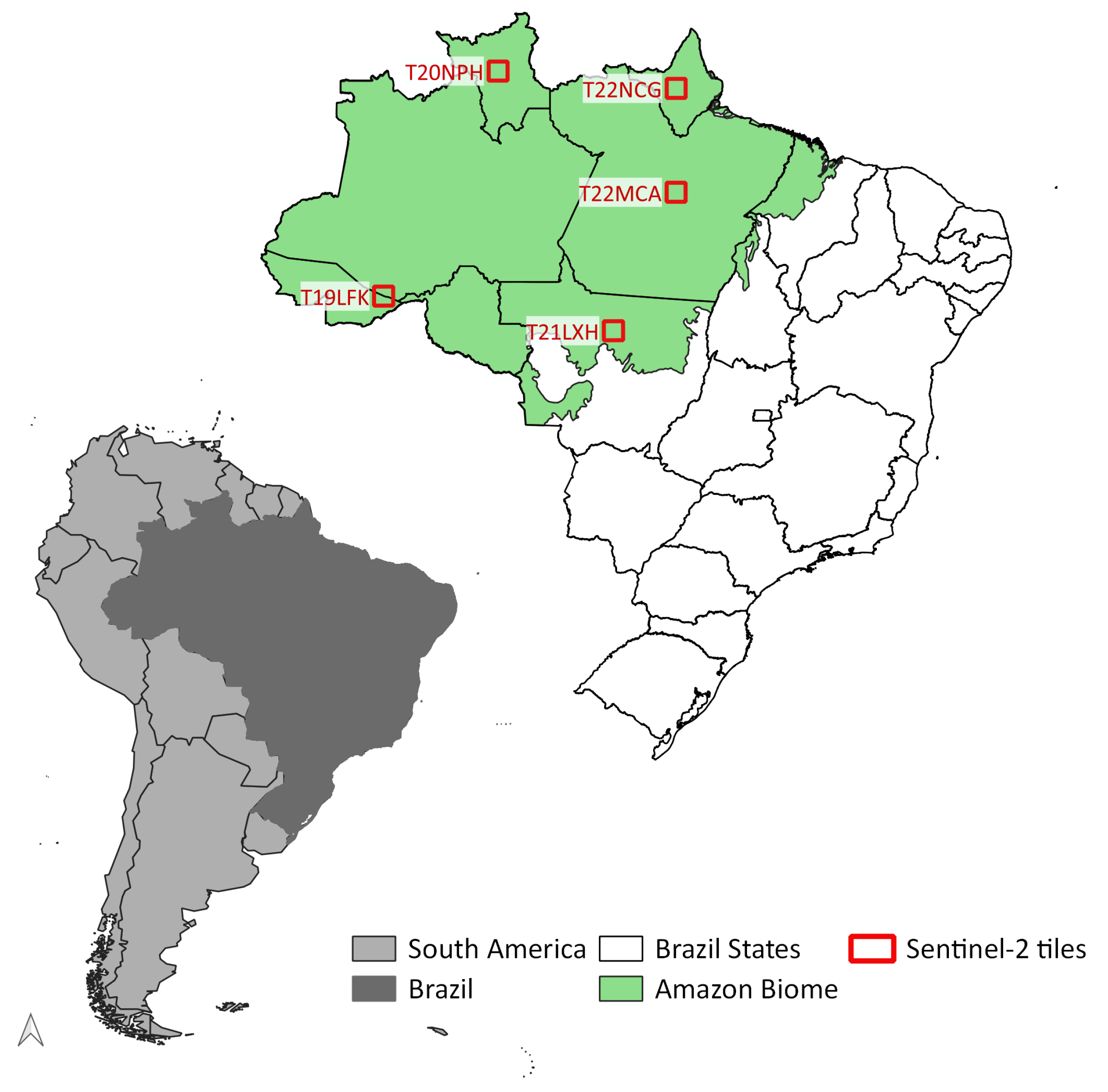
2.1. Study Area

The Amazon forest covers half of Brazil (49.3%) and provides four-fifths of its groundwater (81%) with an average rainfall of approximately 2300 mm per year [37]. Persistent cloud cover in Amazonia is a significant limitation for deforestation monitoring by satellite. Using the Landsat archive from 1984 to 1997, Asner [31] shows how the probability of cloud cover on Landsat images depends not only on the month of the year but also on its location inside Amazonia. From June to August, the chance of finding one image with less than 30% cloud cover is 60–90% in southeastern Amazonia. In the southwestern part, cloud cover is persistent all year round. While the recent availability of medium-resolution (10–100 m) sensors with higher temporal frequency than Landsat has improved the chances of obtaining cloud-free pixels, cloud cover in rain forests such as Amazonia will always be a challenge for optical remote sensing.

2.2. Data Selection

This study uses images from the Sentinel–2A satellite, launched in 2015. The satellite is part of the Copernicus Earth Observation program of the European Union, which is operated by the European Space Agency (ESA) and managed by the European Commission. It carries the Multispectral Instrument (MSI), which detects 13 bands of the electromagnetic spectrum spanning from the visible to the short infrared (SWIR) wavelengths at spatial resolutions of 10 m, 20 m, and 60 m, with a revisit period of 10 days [15] (see

Table 1. Sentinel-2 spatial, spectral, and temporal resolution. Source [39].

Band	Resolution (m)	Wavelength (nm)	Revisit Period (Days)
B01 Coastal aerosol	60	443	10
B02 Blue	10	490	10
B03 Green	10	560	10
B04 Red	10	665	10
B05 Vegetation red edge	20	705	10
B06 Vegetation red edge	20	740	10
B07 Vegetation red edge	20	783	10
B08 NIR	10	842	10
B8A Vegetation red edge	20	865	10
B09 Water vapour	60	945	10
B10 SWIR - Cirrus	60	1375	10
B11 SWIR	20	1610	10
B12 SWIR	20	2190	10

). MSI’s three bands at 60 m resolution are dedicated to atmospheric correction and cloud screening, leaving ten bands for land observation [38]. Sentinel-2A data enables researchers to explore the changes on Earth’s surface due to its open data access policy and its temporal, spatial, and spectral resolutions.

To assess cloud detection algorithms over Amazonia, we chose five areas representative of its climate heterogeneity. We identify them using the tiling system of Sentinel–2:

T19LFK: 

Covers part of the states of Acre and Amazonas, including an indigenous land (Terra Indígena Apurianã) and a protected area (Reserva Extrativista Chico Mendes). The region is associated with significant recent deforestation.

T20NPH: 

This area is in the state of Roraima and it partially covers a national forest (Floresta Nacional de Roraima) and an indigenous land (Terra Indígena Yanomami).

T21LXH: 

This area covers part of the state of Mato Grosso; it includes fragmented forest areas, soybean crops, pasture, and water reservoirs.

T22MCA: 

In the state of Para, this area overlaps various indigenous reserves (Arara, Araweté, Kararaô, Koatinemo, and Trincheira) and part of a conservation unit; most of the area is covered by native forest with some deforested areas to the North.

T22NCG: 

This area is in the state of Amapá, including part of a National Forest (Amapá), a national park (Montanhas do Tumucumaque), and an indigenous land (Waiãpi).

Tiles T21LXH and T18LFK represent areas where most of the deforestation in Amazonia occurred since the 1970s. Tile T21LXH is a hotspot of Brazil’s agricultural frontier with a well-defined dry season from July to September. Tile T18LFK is under the direct influence of the urban area of Rio Branco, the capital of Acre, including both deforestation and protected areas. Deforestation has increased recently in the region of tile T22MCA, threatening indigenous lands. Unlike the others, tiles T20NPH and T22NCG are in the Northern hemisphere, where the seasons and cloud patterns differ from areas to the south of the Equator. Tile T22NCG has much cloud cover all year round and low deforestation. Tile T20NPH overlaps forest and natural savanna, where emerging mining activities are menacing indigenous territories (Figure 1).

2.3. Cloud Detection Algorithms

The paper compares four algorithms: Fmask 4 [25], MAJA [23], Sen2Cor 2.8 [22], and S2cloudless [27]. Fmask 4 and s2cloudless are specific for cloud detection. MAJA and Sen2Cor 2.8 are image processors; they generate cloud masks as part of image conversion from radiance at the top of the atmosphere to reflectance from ground targets. To process Landsat 8 data, USGS uses a version of the Fmask method that requires the thermal band [40]. Fmask 4 is a version of Fmask that has been adjusted to be used with sensors without thermal bands. ESA uses Sen2Cor to process Sentinel–2 images. MAJA is developed by CNES and is used by applications such as Sen2Agri [41]. The Sentinel Hub uses S2cloudless for the fast generation of cloud masks [27]. These methods represent the latest generation of cloud detection algorithms for optical remote sensing images.

Fmask 4 [25] is the most recent version of Fmask [20]. Earlier versions of Fmask required a thermal band and worked only on Landsat images. The latest version also works on Sentinel–2 images [25]. To distinguish between clouds and bright surfaces in Landsat 8 images, Fmask 4 uses the thermal band. In the case of Sentinel–2 images, it takes the view angle parallax of the NIR bands [24]. To reduce false positives resulting from snow and built-up areas, Fmask 4 uses spectral and contextual features. To distinguish land from water, it relies on global surface water map [42]. Fmask 4 matches clouds with their shadows based on similarity. It iterates cloud height from a minimum to a maximum level; for each possible height, it computes the similarity between cloud and cloud shadows [43]. When processing Sentinel–2 images, its cloud and cloud shadow masks have a 20 m resolution [25].

Sen2Cor processes Sentinel–2 data to estimate Bottom-Of-Atmosphere (BOA) reflectances from Top-Of-Atmosphere (TOA) data [22]. It takes Level-1C images and adjusts for atmospheric effects, generating Level-2A surface reflectance products [22,39]. It generates two types of results: (1) atmospheric correction products, such as aerosol optical thickness, surface reflectance, and water vapor maps; and (2) cloud screening and scene Classification (SCL), which assigns a class to each pixel. Sen2Cor provides two quality indicators: A cloud confidence map and a snow confidence map with values ranging from 0 to 100%. The distinction between cloudy, clear and water pixels in the SCL and the output of the cloud confidence map are used to produce the cloud confidence information [39]. The current version of Sen2Cor (2.8) increases the accuracy of classification on water, urban, and bare areas while reducing false positives for snow. Other improvements include cirrus detection, false cloud detection due to permanent bright targets, classification of water pixels inside of cloud borders, and discrimination between topographic and cloud shadow pixels [44].

Sentinel Hub’s S2cloudless is a machine-learning-based cloud detector [27]. Its input is Level-1C top of atmosphere data from 10 Sentinel–2 bands (bands 1-5 and 8-12) combined with pairwise band differences and band ratios. It uses the LightGBM algorithm [45] trained over multiple clouded and non-clouded samples over the world. As training data, is uses cloud masks provided by MAJA as a proxy for ground truth. S2cloudless trained its classification model with $\mathrm{15,000}$ Sentinel–2 tiles from 596 geographically unique areas in 77 different countries.

MAJA (MACCS–ATCOR Joint Algorithm) combines two methods: (a) the Multi-sensor Atmospheric Correction and Cloud Screening (MACCS) and (b) the Atmospheric and Topographic Correction (ATCOR). It builds on these methods by including time-series of images to improve detection of reflectance changes due to clouds [46]. The method assumes that surface reflectances without clouds are stable in time, while clouds or cloud shadows result in quick variations [23]. MAJA uses multi-temporal images that contain the most recent cloud-free observation for each pixel. At each new image, the algorithm updates this composite with the newly-available cloud-free pixels. Thus, it processes the data for a given location in chronological order [26]. The algorithm needs to be initialized to fix cases where a given pixel has no cloud-free observations. To cover these specific cases, MAJA also uses a mono-temporal criterion based only on spectral information [23].

2.4. Algorithm Configuration

To run Fmask 4, MAJA 3.2.2, and Sen2Cor 2.8, we used Linux Docker containers. The Fmask 4 implementation uses the MATLAB code available at GitHub (https://github.com/GERSL/Fmask). For Sen2Cor 2.8, we installed the version provided by ESA (https://step.esa.int/main/third-party-plugins-2/sen2cor/). The MAJA implementation was obtained from CNES (https://logiciels.cnes.fr/fr/content/maja). We downloaded S2cloudless 1.4.0 from the Sentinel Hub (https://www.sentinel-hub.com/). Run-time parameters are described below.

Fmask 4: 

Dilation parameters for cloud, cloud shadows, and snow were set to 3, 3, and 0 pixels, respectively. The cloud probability threshold was 20%, following Qiu et al. [47].

S2cloudless: 

Cloud probability threshold was set to 70%, using a four-pixel convolution for averaging cloud probabilities and dilation of two pixels, following the parameters set by Zupanc et al. [27].

Sen2Cor 2.8: 

The tests used the same configuration as that of the Land Cover maps of ESA’s Climate Change Initiative (http://maps.elie.ucl.ac.be/CCI/viewer/download.php).

MAJA: 

The evaluation used the same configuration as that of the Sen2Agri application (http://www.esa-sen2agri.org).

2.5. Validation Sample Set

To validate the resulting cloud masks, we used sample points tagged by remote sensing experts through visual interpretation, following the work of Foga et al. and Zhu et al. [36,40]. We selected a set of random locations inside each Sentinel–2 tile. Since Sentinel–2 images at 10 m resolution have over 120 million pixels, standard statistical techniques indicate that using about 400 samples per image is enough to achieve a 95% confidence level with a 5% margin of error [48]. Five experts labeled those points in all 20 images. The labels were “cloud”, “cloud shadow”, “clear”, and “other”. The “other” label is a placeholder for samples that the experts could not tag. Since the areas of cloud shadow are small compared to other labels, we tried to ensure there were at least 50 samples of cloud shadows. Two different experts classified each point; only those where both experts agreed were selected. Because of the need for agreement between experts, the final number of selected samples changes from image to image (see

Table 2. Number of samples per image in which two experts agreed.

Tile	Date	Samples
T19LFK	4 October 2016	382
T19LFK	2 January 2017	437
T19LFK	7 May 2018	392
T19LFK	3 November 2018	452
T20NPH	1 September 2016	326
T20NPH	10 November 2016	246
T20NPH	18 February 2017	353
T20NPH	18 July 2017	311
T21LXH	28 March 2017	496
T21LXH	11 June 2018	474
T21LXH	19 September 2018	436
T21LXH	9 October 2018	457
T22MCA	3 June 2017	368
T22MCA	23 June 2017	404
T22MCA	19 April 2018	445
T22MCA	28 June 2018	447
T22NCG	29 September 2016	464
T22NCG	19 October 2016	426
T22NCG	27 May 2017	346
T22NCG	6 July 2017	433

).

2.6. Label Compatibility

Since the algorithms tested use different labels, we recoded their results to match the labels in the validation sample set. In particular, MAJA produces an 8-bit mask, so that many labels can be applied to a pixel, allowing combinations that are not available in the results of other algorithms. For example, MAJA’s mask allows tagging a pixel as a shadow projected on top of a cloud from another cloud in a neighboring image. To make MAJA’s more detailed results compatible with the output of the other methods, we prioritize clouds over cloud shadows and cloud shadows over clear pixels.

Table 3. Label recoding of the detection algorithms.

Expert label	Fmask4	MAJA	s2cloudless	Sen2Cor
Clear	0 Clear land	0–1 Clear	0 Clear	4 Vegetation
	1 Clear water			5 Non vegetated
	3 Snow			6 Water
				11 Snow
Cloud	4 Cloud	2–3 Cloud	1 Cloud	8 Cloud medium probability
		6–7 Cloud		9 Cloud high probability
		10–11 Cloud		10 Thins cirrus
		14–63 Cloud
		64–127 Cirrus
		128–191 Cloud
		192–255 Cirrus
Cloud shadow	2 Cloud shadow	4–5 Cloud shadow		2 Dark area pixels
		8–9 Cloud shadow		3 Cloud shadows
		12–13 Cloud shadow
Other				0 No data
				1 Saturated or defective
				7 Unclassified

shows how the original codes for each method were relabelled for compatibility.

2.7. Validation Metrics

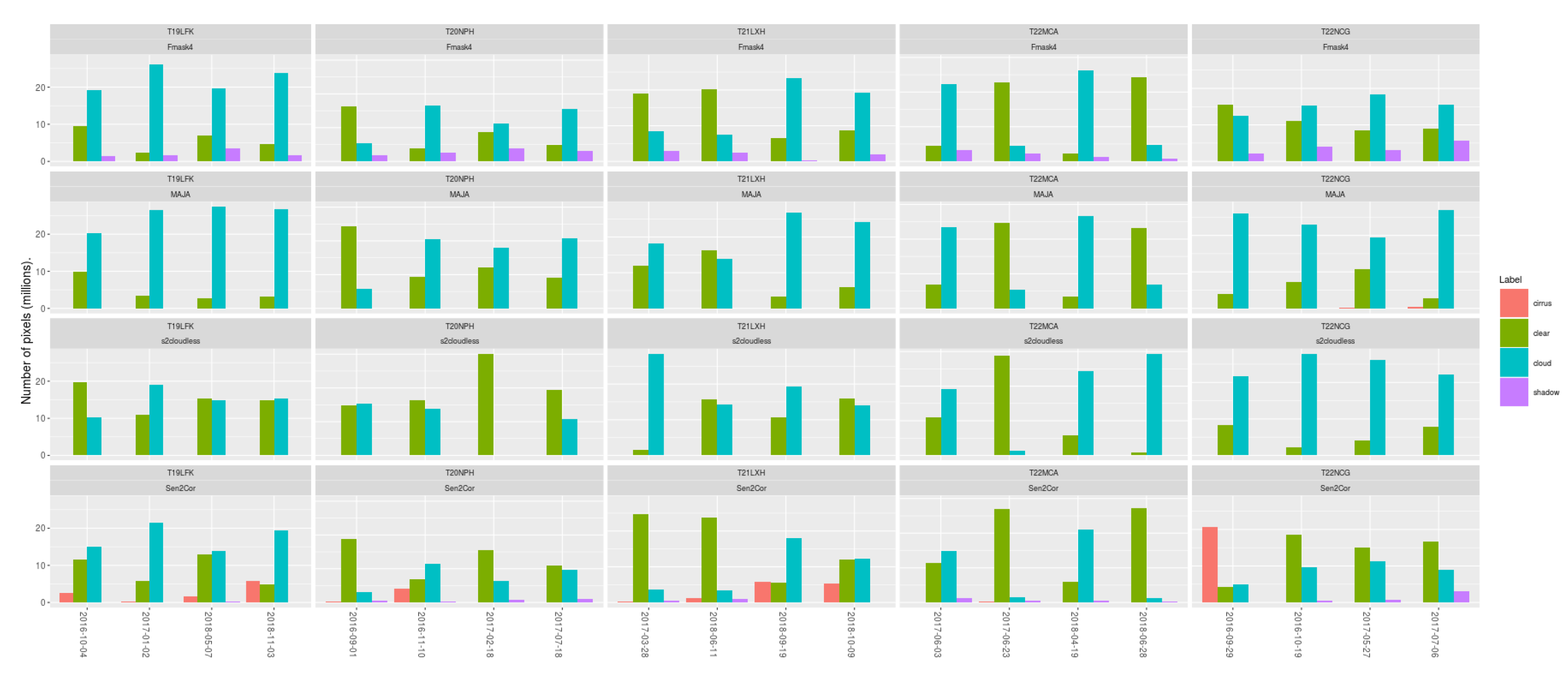
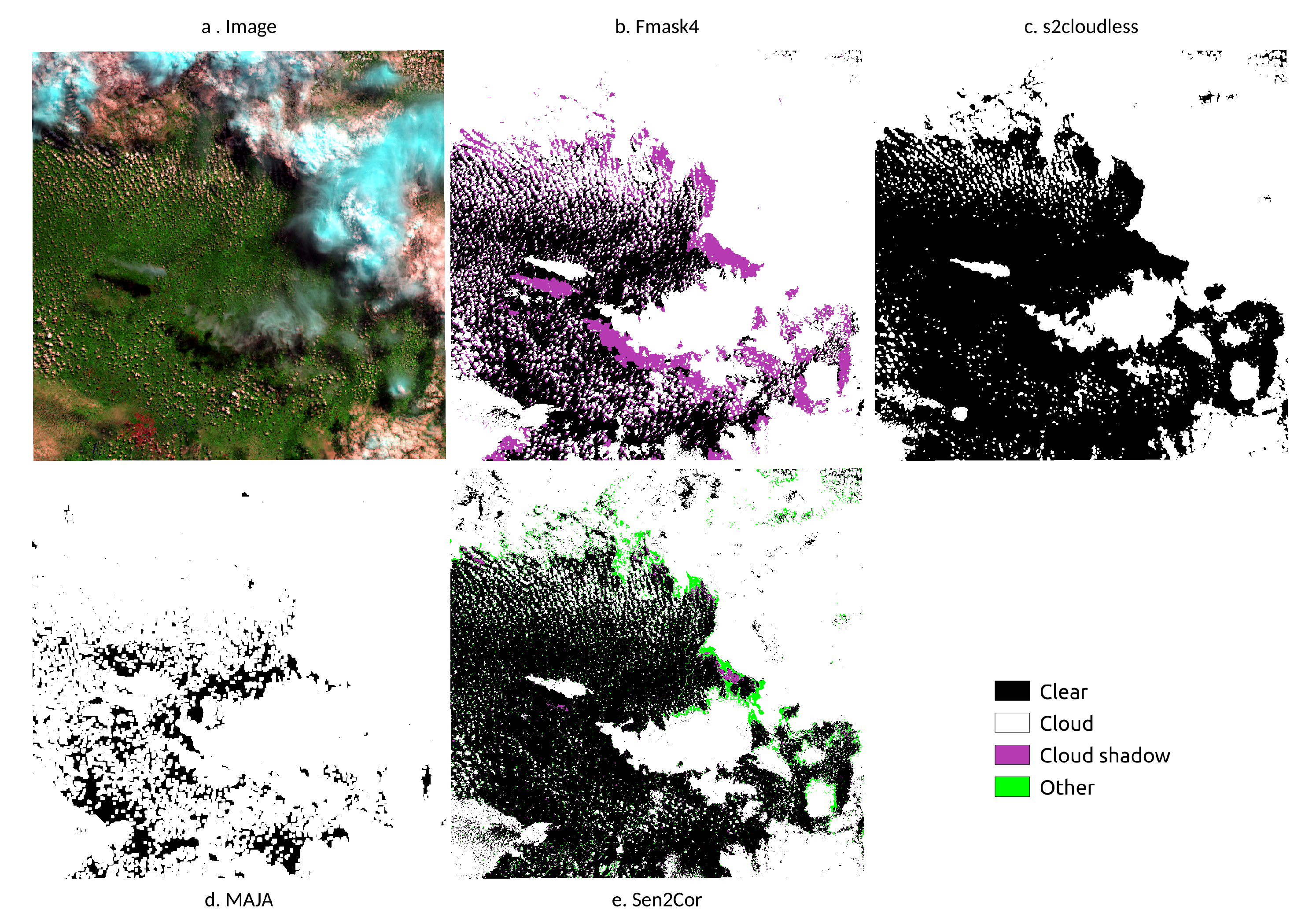
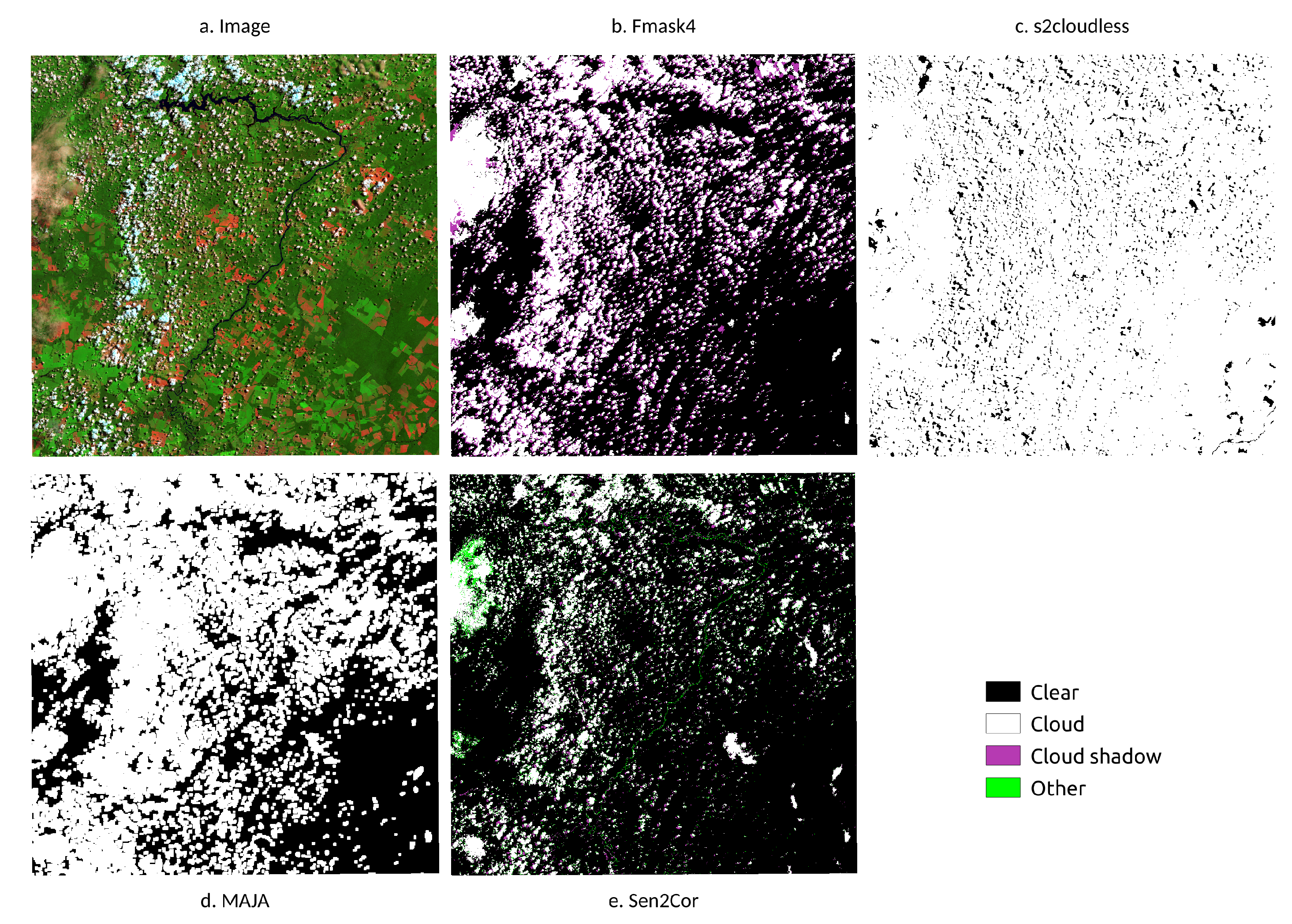
To compare the results of the algorithms, we use the F1 score [49] and the user’s, producer’s, and overall accuracies [50]. The F1 score (Equation (1)) is the harmonic mean of the precision (Equation (2)) and recall rates (Equation (3)). The producer’s accuracy measures how well a certain label has been classified. It is computed by dividing the correctly classified pixels in each class by the total number of pixels of the corresponding class. The user’s accuracy indicates the probability that prediction represents reality. It is computed by dividing the correctly classified pixels in each label by the total number of pixels classified in that label. The overall accuracy indicates the quality of the map classification. It is calculated by dividing the total number of correctly classified pixels by the total number of reference pixels.

$$F1score=2\times \frac{Precision\times Recall}{Precision+Recall}$$

(1)

$$Precision=\frac{TruePositives}{TruePositives+FalseNegatives}$$

(2)

$$Recall=\frac{TrueNegatives}{TrueNegatives+FalsePositives}$$

(3)

3. Results

In our experiments, Fmask 4 has the best overall accuracy, followed by Sen2Cor, MAJA, and S2cloudless (see

Table 4. F1 scores, user, and producer accuracies for each cloud detection algorithm.

	Fmask 4			MAJA			s2cloudless			Sen2Cor
Label	F1	User	Prod	F1	User	Prod	F1	User	Prod	F1	User	Prod
Clear	0.90	0.90	0.89	0.73	0.82	0.66	0.44	0.42	0.46	0.77	0.67	0.89
Cloud	0.94	0.91	0.96	0.77	0.64	0.97	0.66	0.59	0.75	0.89	0.90	0.88
C. Shadow	0.79	0.84	0.75			0.00			0.00	0.50	0.95	0.34
Overall	0.90			0.69			0.52			0.79

). Fmask 4 consistently outperforms the other algorithms in overall, user’s and producer’s accuracies for all classes. It also has the best results considering individual tiles. For cloud shadow detection, Fmask 4 has a better performance than Sen2Cor. Although MAJA has the ability to detect cloud shadows, in practice the methods extend its cloud mask to include shadows. MAJA is a conservative method that uses dilation operators to improve the user’s accuracy of the clear sky. Therefore, no shadows are reported by MAJA. This is observable in either the images themselves or Figure 2, in which MAJA consistently detects more cloud pixels than the other methods. Furthermore, Fmask 4 and Sen2Cor also distinguish cirrus clouds from clouds, as shown in Figure 2. For accuracy assessment, we merged both types of clouds for computing the information in Table 4 and

Table 5. User and producer accuracies for each tile and cloud-detection algorithm.

		Fmask 4			MAJA			s2cloudless			Sen2Cor
Tile	Label	F1	User	Prod	F1	User	Prod	F1	User	Prod	F1	User	Prod
T19LFK	Clear	0.83	0.81	0.86	0.66	0.69	0.63	0.47	0.31	0.94	0.66	0.52	0.92
	Cloud	0.96	0.96	0.96	0.90	0.85	0.97	0.77	0.94	0.66	0.94	0.96	0.92
	C. Shadow	0.68	0.71	0.66			0.00			0.00			0.00
	Overall	0.92			0.82			0.64			0.84
T20NPH	Clear	0.91	0.95	0.88	0.78	0.89	0.70	0.53	0.47	0.62	0.84	0.73	1.00
	Cloud	0.95	0.90	1.00	0.71	0.56	0.98	0.57	0.54	0.60	0.93	0.99	0.88
	C. Shadow	0.80	0.82	0.78			0.00			0.00	0.59	1.00	0.42
	Overall	0.91			0.67			0.50			0.84
T21LXH	Clear	0.88	0.82	0.95	0.80	0.89	0.72	0.35	0.33	0.36	0.78	0.64	0.99
	Cloud	0.94	0.96	0.92	0.77	0.64	0.98	0.60	0.52	0.70	0.91	0.99	0.83
	C. Shadow	0.81	0.89	0.75			0.00			0.00	0.58	0.98	0.41
	Overall	0.90			0.71			0.45			0.81
T22MCA	Clear	0.94	0.94	0.94	0.88	0.83	0.93	0.58	0.62	0.54	0.85	0.74	0.98
	Cloud	0.94	0.90	0.98	0.82	0.71	0.97	0.70	0.56	0.93	0.95	1.00	0.90
	C. Shadow	0.81	0.89	0.74			0.00			0.00	0.49	0.87	0.34
	Overall	0.92			0.77			0.58			0.83
T22NCG	Clear	0.87	0.95	0.80	0.42	0.70	0.30	0.23	0.34	0.18	0.63	0.64	0.63
	Cloud	0.87	0.79	0.96	0.58	0.43	0.92	0.61	0.46	0.94	0.71	0.62	0.83
	C. Shadow	0.80	0.82	0.77			0.00			0.00	0.53	0.97	0.36
	Overall	0.86			0.48			0.43			0.65

to be able to compare Fmask 4 and Sen2Cor with the other methods.

When comparing the overall accuracy of Sen2Cor with that of MAJA, their design choices stand out. MAJA has a better user’s accuracy for clear sky pixels than Sen2Cor; for producer’s accuracy of this class, Sen2Cor is superior. Conversely, MAJA has a better producer’s accuracy than Sen2Cor for cloud pixels; for the user’s accuracy, the situation is inverted. This situation also holds in individual tiles (see Table 5). The designers of MAJA have chosen to maximize the probability that pixels labeled as a clear sky are correct.

The behavior of S2cloudless is erratic; sometimes it produces results visually similar to those of Fmask 4 or Sen2Cor (see Figure 3), while in some other occasions it misclassifies clear pixels as clouds (see Figure 2). For example, for tile T21LXH on 28 March 2017 and tile T22MCA on 28 June 2018, S2cloudless has a particularly poor performance. Figure 4 shows tile T21LXH on 28 March 2017, a case where S2cloudless performs differently from the other methods.

These results showed that the four algorithms produce their best results on images with few well-defined (crisp) clouds. Except for s2cloudless, the algorithms agree on the shape and the number of areas classified as either cloud or clear. However, they cannot adequately approximate the shape of clouds and their shadows on thin semi-transparent cirrus or tightly packed clouds (see Figure 5). The accurate detection of cloud shadows is challenging because dark surfaces, such as wetlands, burned areas, and terrain shadows can be easily confused with cloud shadows [25].

The pictures shown in Figure 4 confirm the results discussed above. While Fmask4 has the best performance, it is interesting to compare MAJA with Sen2Cor. MAJA uses squircles (i.e., a shape between a circle and a rectangle) to fill in the cloud shape, ensuring the total coverage of each cloud in detriment of cloud shadows. Thus, MAJA sometimes incorporates clear pixels in its cloud mask, as also reported by [26]. By contrast, Sen2Cor approximates the shape of the cloud from the inside, filling in the clouds’ boundaries with saturated labels—particularly with thin cirrus clouds—which produces rough borders (see Figure 5). Furthermore, Sen2Cor cannot detect small clouds which are correctly identified by Fmask 4 and MAJA (e.g., see the small clouds at the center of Figure 3).

The shadow masks produced by Fmask 4 are displaced regarding to the shadows visible in the images. This is a consequence of the coarse spatial resolution of the digital elevation model used by the method. As for their shapes, Fmask 4 matches well the cloud shadows respect to the clouds producing them, while in Sen2Cor the cloud shadows have smoother and different boundaries than their clouds (see Figure 5). Our results confirm the work of Qiu et al. [25] and Baetens et al. [26], who report that Fmask 4 works better in detecting clouds and cloud shadows than Sen2Cor for Sentinel–2A images.

We could not compute the accuracies for cloud shadow detection for MAJA and S2cloudless. This is expected from s2cloudless but it comes as a surprise in the case of MAJA. An explanation is MAJA’s greedy behavior regarding clouds; it tends to tag pixels as clouds in disregard of their shadows (see Figure 2). An alternative explanation is due to our interpretation of the MAJA’s bit mask where we prioritized clouds over cloud shadows (see Section 2.6).

Sen2Cor tags many pixels as saturated, defective, or unclassified which we labelled as other (see Table 3). A visual inspection reveals most of the saturated pixels are the external border of clouds (see Figure 3). On the other hand, Sen2Cor in tile T21LXH for 08 March 2017 (see Figure 4) mistakenly displays cloud and cloud shadow pixels along the riverbank, almost perfectly profiling the whole river; this could be caused by suspended matter in the water. Sen2Cor problems to detect cloud cover over water were also reported by [25,51]. As discussed above, the shapes of clouds in the Sen2Cor mask are rougher compared to the smoother results using the other algorithms. Despite these issues, Sen2Cor is a reliable method for cloud detection. Its producer’s accuracies for clear sky and clouds are respectively 89% and 88%. If its errors in detecting cloud shadows can be tolerated by the user, its efficiency and ease of use may justify its choice for bulk processing.

S2cloudless erratically mixes land features and clouds, particularly on images with few clouds. It does not spot cloud shadows. We could not confirm the claims made by the authors of this method [27] about the good performance of this algorithm. One explanation is that the clouds in tropical forests such as Amazonia are not adequately included in the S2cloudless training set.

4. Discussion

The results of this study show that the Fmask 4 algorithm consistently performs better than the alternatives for Sentinel-2 images of the Amazon rain forest. Fmask 4 had an overall accuracy of 90%, followed by Sen2Cor (79%), MAJA (69%) and s2cloudless (52%). Our results are different from those of Baetens et al. [26] who concluded that MAJA and Fmask 4 perform similarly with an overall accuracy around 90%, while Sen2Cor had an overall accuracy of 84%. We now consider some hypothesis that could account for such significant differences.

As noted by Baetens et al. [26], for satellites without thermal bands cloud detection methods use thresholds. Different thresholds are set for the visible bands, the $1.38$ $\mathsf{\mu }$$\mathrm{m}$ band, and the Normalized Difference Snow Index. These approximations address important challenges for cloud detection methods: distinguishing clouds from snow, mountain tops, bright deserts, and large built-up objects. Since each cloud detection method relies on different ad hoc hypotheses, its usefulness varies from scene to scene. For this reason, no single study can provide definitive guidance. Studies that target specific regions, such as the current paper, provide valuable advice even though its results cannot be generalized to non-forest areas.

The comparison done by Baetens et al. [26] uses 10 different sites, including equatorial forests, deserts and semi-deserts, agricultural areas, mountains, and snowy areas. Their results provide a balance between different targets that could be confused with clouds. By contrast, our study deals only with forest and agriculture areas; the images tested have no deserts, mountains or snow. By focusing on the Amazon biome, our results are intended as guidance for experts interested in measuring land change in the region. Given its focus, these results cannot be generalized to non-forest regions.

A further consideration that could explain part of the differences between our work and that of Baetens et al. [26] is the choice of training data sets. While we use random sampling, those authors preferred to rely on active learning. An active learning model uses a few good quality samples instead of a large ensemble of random points. These good quality samples are used to train a machine learning model (random forest) whose output provides labels to a large set point for classification. In theory, this method has the advantage of being able to provide a larger number of points to test the algorithm. Machine learning models have a tendency to overfit their training data, which could cause wrong predictions [52]. The alternative is to use random samples, which rely on standard statistical assumptions. However, random samples can miss some cloud properties. Clouds come in different shapes, sizes, and transparencies; it is often hard to distinguish overlapping clouds at different heights from images. Random samples can also misrepresent minority labels such as cloud shadows. Therefore, both random sampling and active learning have their advantages and shortcomings for evaluating cloud detection algorithms. Further testing and comparison are required to evaluate these approaches.

Another source of divergence between our result and that of Baetens et al. [26] is due to class relabeling. Cloud detection algorithms codify their results using different levels of detail. To enable comparisons, we had to recode them to the same set of labels. This process implies a loss of information, in particular for MAJA, which provides the most detailed data about its detection process. Thus, our recoding process could have had a negative impact on our evaluation of MAJA.

Despite the differences discussed above, there are points of convergence between our work and earlier papers such as Baetens et al. [26] and Qiu et al. [25] related to Fmask 4 performance. The overall user’s and producer’s accuracy values for Fmask 4 are broadly consistent in the three studies. Qiu et al. [25] report producer’s accuracies for clouds, shadows and clear pixels to be 93%, 70%, and 97%, while our results are 96%, 75%, and 90%. Thus, we consider that Fmask 4 to be a reliable method that we recommend to be used for cloud detection in Sentinel-2 images of the Amazon rain forest.

5. Conclusions

In this work, we compared four cloud detection algorithms on Sentinel–2A images of the Amazon tropical forest, and we found that Fmask 4 performs the best. We tested four cloud detection algorithms—FMask 4, Sen2Cor, MAJA, and S2cloudless—on 20 images with a different amount of cloud coverage, spread over five regions of Amazonia. We validated the results of the cloud detection algorithms using the criteria of experts on remote sensing who classified approximately 400 random points on each image. To determine the best algorithm, we computed the F1 score and the overall, user, and producer accuracies. We found that FMask 4 has an overall accuracy of 90% to detect clouds, while Sen2Cor’s OA is 79%, MAJA’s OA is 69%, and S2cloudless’s OA is 52%. Based on these results, we recommend the use of Fmask 4 for cloud detection of Sentinel-2 images of the Amazon region.

The choice of method depends on the intended use. Therefore, users should consider the benefits of each method before making their choices. Since MAJA reduces the number of false positives by design, users that aim to improve the producer’s accuracy should consider its use. These characteristics could make MAJA suitable, for example, to build cloud-free monthly mosaics. Despite the poor performance of S2cloudless in our study, we consider that the use of machine learning methods for cloud detection is a promising way forward. As more good quality samples become available, its performance will improve. Finally, Sen2Cor is an efficient method to detect clouds in Sentinel-2 images. Despite not having the best performance, its ease of use may appeal to those that need fast processing of large data sets.

We expect our work to impact on the building of data cubes of analysis-ready data from satellite imagery, like those currently under construction by the Brazil Data Cube project. (Brazil Data Cube project http://brazildatacube.org/) Another application is for improving the time series analysis of Land Use and Land Cover change of deforested areas, which is particularly hard because of cloud coverage. Given the performance of FMask 4, space agencies and committees such as CEOS should consider the value of working together to develop a standardized best quality cloud detection methods that could be shared and used for remote sensing optical imagery.

The R and Python scripts used to compare the performance of cloud detection algorithms are available on GitHub: https://github.com/brazil-data-cube/compare-cloud-masks.

References

1. Antonelli, A.; Zizka, A.; Carvalho, F.A.; Scharn, R.; Bacon, C.D.; Silvestro, D.; Condamine, F.L. Amazonia Is the Primary Source of Neotropical Biodiversity. Proc. Natl. Acad. Sci. USA 2018, 115, 6034–6039. [Google Scholar] [CrossRef] [PubMed] [Green Version]
2. Ometto, J.; Aguiar, A.; Assis, T.; Soler, L.; Valle, P.; Tejada, G.; Lapola, D.; Meir, P. Amazon Forest Biomass Density Maps: Tackling the Uncertainty in Carbon Emission Estimates. Clim. Chang. 2014, 124, 545–560. [Google Scholar] [CrossRef]
3. Gibbs, H.K.; Ruesch, A.S.; Achard, F.; Clayton, M.K.; Holmgren, P.; Ramankutty, N.; Foley, J.A. Tropical Forests Were the Primary Sources of New Agricultural Land in the 1980s and 1990s. Proc. Natl. Acad. Sci. USA 2010, 107, 16732–16737. [Google Scholar] [CrossRef] [PubMed] [Green Version]
4. INPE. Amazon Deforestation Monitoring Project (PRODES); Technical Report; National Institute for Space Research: São José dos Campos, Brazil, 2019. [Google Scholar]
5. Nepstad, D.; McGrath, D.; Stickler, C.; Alencar, A.; Azevedo, A.; Swette, B.; Bezerra, T.; DiGiano, M.; Shimada, J.; Seroa da Motta, R.; et al. Slowing Amazon Deforestation through Public Policy and Interventions in Beef and Soy Supply Chains. Science 2014, 344, 1118–1123. [Google Scholar] [CrossRef] [PubMed]
6. Soterroni, A.C.; Mosnier, A.; Carvalho, A.X.Y.; Camara, G.; Obersteiner, M.; Andrade, P.R.; Souza, R.C.; Brock, R.; Pirker, J.; Kraxner, F.; et al. Future Environmental and Agricultural Impacts of Brazil’s Forest Code. Environ. Res. Lett. 2018, 13, 074021. [Google Scholar] [CrossRef] [Green Version]
7. Shimabukuro, Y.E.; Santos, J.R.; Formaggio, A.R.; Duarte, V.; Rudorff, B.F.T. The Brazilian Amazon Monitoring Program: PRODES and DETER Projects. In Global Forest Monitoring From Earth Observation; Taylor and Francis: New York, NY, USA, 2012; 354p. [Google Scholar]
8. Assuncao, J.; Gandour, C.; Rocha, R. Deforestation Slowdown in the Brazilian Amazon: Prices or Policies? Environ. Dev. Econ. 2015, 20, 697–722. [Google Scholar] [CrossRef] [Green Version]
9. Gibbs, H.K.; Rausch, L.; Munger, J.; Schelly, I.; Morton, D.C.; Noojipady, P.; Soares-Filho, B.; Barreto, P.; Micol, L.; Walker, N.F. Brazil’s Soy Moratorium. Science 2015, 347, 377–378. [Google Scholar] [CrossRef]
10. Almeida, C.; Coutinho, A.; Esquerdo, J.; Adami, M.; Venturieri, A.; Diniz, C.; Dessay, N.; Durieux, L.; Gomes, A. High Spatial Resolution Land Use and Land Cover Mapping of the Brazilian Legal Amazon in 2008 Using Landsat-5/TM and MODIS Data. Acta Amaz. 2016, 46, 291–302. [Google Scholar] [CrossRef]
11. Souza, C., Jr.; Siqueira, J.; Sales, M.; Fonseca, A.; Ribeiro, J.; Numata, I.; Cochrane, M.; Barber, C.; Roberts, D.; Barlow, J. Ten-Year Landsat Classification of Deforestation and Forest Degradation in the Brazilian Amazon. Remote Sens. 2013, 5, 5493–5513. [Google Scholar] [CrossRef] [Green Version]
12. Tyukavina, A.; Hansen, M.C.; Potapov, P.V.; Stehman, S.V.; Smith-Rodriguez, K.; Okpa, C.; Aguilar, R. Types and Rates of Forest Disturbance in Brazilian Legal Amazon, 2000–2013. Sci. Adv. 2017, 3, e1601047. [Google Scholar] [CrossRef] [PubMed] [Green Version]
13. Hansen, M.C.; Potapov, P.V.; Moore, R.; Hancher, M.; Turubanova, S.A.; Tyukavina, A.; Thau, D.; Stehman, S.V.; Goetz, S.J.; Loveland, T.R.; et al. High-Resolution Global Maps of 21st-Century Forest Cover Change. Science 2013, 342, 850–853. [Google Scholar] [CrossRef] [PubMed] [Green Version]
14. Picoli, M.; Camara, G.; Sanches, I.; Simoes, R.; Carvalho, A.; Maciel, A.; Coutinho, A.; Esquerdo, J.; Antunes, J.; Begotti, R.A.; et al. Big Earth Observation Time Series Analysis for Monitoring Brazilian Agriculture. ISPRS J. Photogramm. Remote Sens. 2018, 145, 328–339. [Google Scholar] [CrossRef]
15. Drusch, M.; Del Bello, U.; Carlier, S.; Colin, O.; Fernandez, V.; Gascon, F.; Hoersch, B.; Isola, C.; Laberinti, P.; Martimort, P.; et al. Sentinel-2: ESA’s Optical High-Resolution Mission for GMES Operational Services. Remote Sens. Environ. 2012, 120, 25–36. [Google Scholar] [CrossRef]
16. Griffiths, P.; Linden, S.; Kuemmerle, T.; Hostert, P. A Pixel-Based Landsat Compositing Algorithm for Large Area Land Cover Mapping. IEEE J. Sel. Top. Appl. Earth Obs. Remote Sens. 2013, 6, 2088–2101. [Google Scholar] [CrossRef]
17. Brown, J.C.; Kastens, J.H.; Coutinho, A.C.; Victoria, D.d.C.; Bishop, C.R. Classifying Multiyear Agricultural Land Use Data from Mato Grosso Using Time-Series MODIS Vegetation Index Data. Remote Sens. Environ. 2013, 130, 39–50. [Google Scholar] [CrossRef] [Green Version]
18. Rufin, P.; Mueller, H.; Pflugmacher, D.; Hostert, P. Land Use Intensity Trajectories on Amazonian Pastures Derived from Landsat Time Series. Int. J. Appl. Earth Obs. Geoinf. 2015, 41, 1–10. [Google Scholar] [CrossRef]
19. Jakimow, B.; Griffiths, P.; Linden, S.; Hostert, P. Mapping Pasture Management in the Brazilian Amazon from Dense Landsat Time Series. Remote Sens. Environ. 2018, 205, 453–468. [Google Scholar] [CrossRef]
20. Zhu, Z.; Woodcock, C.E. Object-Based Cloud and Cloud Shadow Detection in Landsat Imagery. Remote Sens. Environ. 2012, 118, 83–94. [Google Scholar] [CrossRef]
21. Claverie, M.; Ju, J.; Masek, J.G.; Dungan, J.L.; Vermote, E.F.; Roger, J.C.; Skakun, S.V.; Justice, C. The Harmonized Landsat and Sentinel-2 Surface Reflectance Data Set. Remote Sens. Environ. 2018, 219, 145–161. [Google Scholar] [CrossRef]
22. Louis, J.; Debaecker, V.; Pflug, B.; Main-Knorn, M.; Bieniarz, J.; Mueller-Wilm, U.; Cadau, E.; Gascon, F. SENTINEL-2 Sen2Cor: L2A Processor for Users. In Proceedings Living Planet Symposium; ESA: Paris, France, 2016; p. 8. [Google Scholar]
23. Hagolle, O.; Huc, M.; Auer, S.; Richter, R.; Richter, R. MAJA Algorithm Theoretical Basis Document. 2017. Available online: https://zenodo.org/record/1209633#.XpdnZvnQ-Cg (accessed on 29 November 2019). [CrossRef]
24. Frantz, D.; Haß, E.; Uhl, A.; Stoffels, J.; Hill, J. Improvement of the Fmask Algorithm for Sentinel-2 Images: Separating Clouds from Bright Surfaces Based on Parallax Effects. Remote Sens. Environ. 2018, 215, 471–481. [Google Scholar] [CrossRef]
25. Qiu, S.; Zhu, Z.; He, B. Fmask 4.0: Improved Cloud and Cloud Shadow Detection in Landsats 4–8 and Sentinel-2 Imagery. Remote Sens. Environ. 2019, 231, 111205. [Google Scholar] [CrossRef]
26. Baetens, L.; Desjardins, C.; Hagolle, O. Validation of Copernicus Sentinel-2 Cloud Masks Obtained from MAJA, Sen2Cor, and FMask Processors Using Reference Cloud Masks Generated with a Supervised Active Learning Procedure. Remote Sens. 2019, 11, 433. [Google Scholar] [CrossRef] [Green Version]
27. Zupanc, A. Improving Cloud Detection with Machine Learning. 2019. Available online: https://medium.com/sentinel-hub/improving-cloud-detection-with-machine-learning-c09dc5d7cf13 (accessed on 29 November 2019).
28. Roberts, G.C.; Andreae, M.O.; Zhou, J.; Artaxo, P. Cloud Condensation Nuclei in the Amazon Basin: “Marine” Conditions over a Continent? Geophys. Res. Lett. 2001, 28, 2807–2810. [Google Scholar] [CrossRef]
29. Poschl, U.; Martin, S.T.; Sinha, B.; Chen, Q.; Gunthe, S.S.; Huffman, J.A.; Borrmann, S.; Farmer, D.K.; Garland, R.M.; Helas, G.; et al. Rainforest Aerosols as Biogenic Nuclei of Clouds and Precipitation in the Amazon. Science 2010, 329, 1513–1516. [Google Scholar] [CrossRef] [Green Version]
30. Artaxo, P.; Rizzo, L.V.; Paixão, M.; De Lucca, S.; Oliveira, P.H.; Lara, L.L.; Wiedemann, K.T.; Andreae, M.O.; Holben, B.; Schafer, J.; et al. Aerosol Particles in Amazonia: Their Composition, Role in the Radiation Balance, Cloud Formation, and Nutrient Cycles. In Amazonia and Global Change; American Geophysical Union (AGU): Washington, DC, USA, 2009; pp. 233–250. [Google Scholar] [CrossRef]
31. Asner, G.P. Cloud Cover in Landsat Observations of the Brazilian Amazon. Int. J. Remote Sens. 2001, 22, 3855–3862. [Google Scholar] [CrossRef]
32. Cecchini, M.A.; Machado, L.A.T.; Andreae, M.O.; Martin, S.T.; Albrecht, R.I.; Artaxo, P.; Barbosa, H.M.J.; Borrmann, S.; Fütterer, D.; Jurkat, T.; et al. Sensitivities of Amazonian Clouds to Aerosols and Updraft Speed. Atmos. Chem. Phys. 2017, 17, 10037–10050. [Google Scholar] [CrossRef] [Green Version]
33. Durieux, L. The Impact of Deforestation on Cloud Cover over the Amazon Arc of Deforestation. Remote Sens. Environ. 2003, 86, 132–140. [Google Scholar] [CrossRef]
34. Wang, J.; Chagnon, F.J.F.; Williams, E.R.; Betts, A.K.; Renno, N.O.; Machado, L.A.T.; Bisht, G.; Knox, R.; Bras, R.L. Impact of Deforestation in the Amazon Basin on Cloud Climatology. Proc. Natl. Acad. Sci. USA 2009, 106, 3670–3674. [Google Scholar] [CrossRef] [Green Version]
35. Sun, L.; Yang, X.; Jia, S.; Jia, C.; Wang, Q.; Liu, X.; Wei, J.; Zhou, X. Satellite Data Cloud Detection Using Deep Learning Supported by Hyperspectral Data. Int. J. Remote Sens. 2020, 41, 1349–1371. [Google Scholar] [CrossRef] [Green Version]
36. Zhu, X.; Helmer, E.H. An Automatic Method for Screening Clouds and Cloud Shadows in Optical Satellite Image Time Series in Cloudy Regions. Remote Sens. Environ. 2018, 214, 135–153. [Google Scholar] [CrossRef]
37. Davidson, E.A.; Araujo, A.C.; Artaxo, P.; Balch, J.K.; Brown, I.F.; Bustamante, M.M.C.; Coe, M.T.; DeFries, R.S.; Keller, M.; Longo, M.; et al. The Amazon Basin in Transition. Nature 2012, 481, 321–328. [Google Scholar] [CrossRef] [PubMed]
38. Wolanin, A.; Camps-Valls, G.; Gomez-Chova, L.; Mateo-Garcia, G.; Tol, C.; Zhang, Y.; Guanter, L. Estimating Crop Primary Productivity with Sentinel-2 and Landsat 8 Using Machine Learning Methods Trained with Radiative Transfer Simulations. Remote. Sens. Environ. 2019. [Google Scholar] [CrossRef]
39. Gascon, F.; Bouzinac, C.; Thepaut, O.; Jung, M.; Francesconi, B.; Louis, J.; Lonjou, V.; Lafrance, B.; Massera, S.; Gaudel-Vacaresse, A.; et al. Copernicus Sentinel-2A Calibration and Products Validation Status. Remote Sens. 2017, 9, 584. [Google Scholar] [CrossRef] [Green Version]
40. Foga, S.; Scaramuzza, P.L.; Guo, S.; Zhu, Z.; Dilley, R.D.; Beckmann, T.; Schmidt, G.L.; Dwyer, J.L.; Joseph Hughes, M.; Laue, B. Cloud Detection Algorithm Comparison and Validation for Operational Landsat Data Products. Remote Sens. Environ. 2017, 194, 379–390. [Google Scholar] [CrossRef] [Green Version]
41. Defourny, P.; Bontemps, S.; Bellemans, N.; Cara, C.; Dedieu, G.; Guzzonato, E.; Hagolle, O.; Inglada, J.; Nicola, L.; Rabaute, T.; et al. Near Real-Time Agriculture Monitoring at National Scale at Parcel Resolution: Performance Assessment of the Sen2-Agri Automated System in Various Cropping Systems around the World. Remote Sens. Environ. 2019, 221, 551–568. [Google Scholar] [CrossRef]
42. Pekel, J.F.; Cottam, A.; Gorelick, N.; Belward, A.S. High-Resolution Mapping of Global Surface Water and Its Long-Term Changes. Nature 2016, 540, 418–422. [Google Scholar] [CrossRef]
43. Zhu, Z.; Wang, S.; Woodcock, C.E. Improvement and Expansion of the Fmask Algorithm: Cloud, Cloud Shadow, and Snow Detection for Landsat 4-7, 8, and Sentinel 2 Images. Remote Sens. Environ. 2015, 159, 269–277. [Google Scholar] [CrossRef]
44. Mueller-Wilm, U. Sen2Cor 2.8 Software Release Note; Technical Report; ESA (European Space Agency) Report: Frascati, Italy, 2019. [Google Scholar]
45. Ke, G.; Meng, Q.; Finley, T.; Wang, T.; Chen, W.; Ma, W.; Ye, Q.; Liu, T.Y. Lightgbm: A Highly Efficient Gradient Boosting Decision Tree. In Advances in Neural Information Processing Systems; Curran Associates Inc.: Lane Red Hook, NY, USA, 2017; pp. 3146–3154. [Google Scholar]
46. Hagolle, O.; Huc, M.; Villa Pascual, D.; Dedieu, G. A Multi-Temporal and Multi-Spectral Method to Estimate Aerosol Optical Thickness over Land, for the Atmospheric Correction of FormoSat-2, LandSat, VENμS and Sentinel-2 Images. Remote Sens. 2015, 7, 2668–2691. [Google Scholar] [CrossRef] [Green Version]
47. Qiu, S.; Zhu, Z.; He, B. Fmask 4.0 Handbook. 2018. Available online: https://drive.google.com/drive/folders/1oVefP9G-TD2vhoCaaKCxQjvAnUlrwB19 (accessed on 1 December 2019).
48. Israel, G.D. Determining Sample Size; Technical Report; University of Florida: Gainesville, FL, USA, 1992. [Google Scholar]
49. Chinchor, N. MUC-4 Evaluation Metrics. In Fourth Message Uunderstanding Conference (MUC-4); Association for Computational Linguistics: Stroudsburg, PA, USA, 1992. [Google Scholar]
50. Story, M.; Congalton, R. Accuracy Assessment: A User’s Perspective. Photogramm. Eng. Remote Sens. 1986, 52, 397–399. [Google Scholar]
51. Segal-Rozenhaimer, M.; Li, A.; Das, K.; Chirayath, V. Cloud Detection Algorithm for Multi-Modal Satellite Imagery Using Convolutional Neural-Networks (CNN). Remote Sens. Environ. 2020, 237, 111446. [Google Scholar] [CrossRef]
52. Hastie, T.; Tibshirani, R.; Friedman, J. The Elements of Statistical Learning. Data Mining, Inference, and Prediction; Springer: New York, NY, USA, 2009. [Google Scholar]
Figure 1. Left: Brazil in South America. Right: Location of the Amazon biome along the Sentinel–2 tiles (A) T19LFK (08/25/2016); (B) T21LXH (01/07/2017); (C) T22MCA (07/13/2017).
Remotesensing 12 01284 g001
Figure 2. Number of pixels classified on each Sentinel–2A image.
Remotesensing 12 01284 g002
Figure 3. Clouds detected on the Sentinel–2A image T19LFK of 7 May 2018. The color picture (a) uses bands 12, 8 and 3.
Remotesensing 12 01284 g003
Figure 4. Clouds detected on the Sentinel–2A image T21LXH of 28 March 2017. The image is composed of bands 12, 8 and 3.
Remotesensing 12 01284 g004
Figure 5. Detail of clouds over Amazonia in Sentinel–2A image T22MCA of 23 June 2017. The image is composed of bands 4, 3 and 2.
Remotesensing 12 01284 g005