2.1 Model description

cGENIE is an Earth system model of intermediate complexity, with a 3D frictional-geostrophic ocean (36×36 equal-area horizontal grid, 16 depth levels), 2D energy–moisture balance atmosphere with prescribed wind fields, and interactive atmospheric chemistry and ocean biogeochemistry. The model code and user handbook can be found in the cGENIE GitHub repository (cGENIE GitHub repository, 2019). We run a version of cGENIE with the same phosphorus-plus-iron (Fe) co-limitation scheme as used in the iron cycle model inter-comparison study of Tagliabue et al. (2016). The model branch enabled for use with flexible C∕P ratios (see Sect. 2.2) is tagged as release v0.9.5, and the model configurations used in this paper are included in this release (cGENIE release v0.9.5, 2019, see Code availability for details).

2.2 Stoichiometry

In the original version of the cGENIE Earth system model (Ridgwell et al., 2007), as well as in the version of Tagliabue et al. (2016), the stoichiometric ratios are based on Redfield (1963). Thus, there is a fixed relationship between the number of moles of the elements that are taken up (positive) or released (negative) during production of organic matter in the ocean. This relationship is $\mathrm{P}/\mathrm{C}/{\mathrm{O}}_{\mathrm{2}}=\mathrm{1}/\mathrm{106}/-\mathrm{138}$, where O₂ is dissolved oxygen (nitrogen is assumed only implicitly for the purpose of accounting for organic matter creation and remineralization-related alkalinity transformations in the ocean; Ridgwell et al., 2007). An exception is iron, where Fe∕C varies as a function of iron availability as described in Watson et al. (2000).

Although the average elemental composition of organic matter in the ocean is close to the Redfield ratios, the stoichiometry of production of new organic material has shown high in situ variability. Variability occurs between species, but also within the same species, and has been shown to depend on environmental factors such as nutrient availability, water temperature, and light (e.g. Le Quéré et al., 2005; Galbraith and Martiny, 2015; Yvon-Durocher et al., 2015; Tanioka and Matsumoto, 2017; Garcia et al., 2018a; Moreno et al., 2018). We test the importance of this variability for glacial ocean CO₂ storage by running the same experiments with the fixed Redfield stoichiometry version of cGENIE and with a model version where we have implemented the linear regression model presented by Galbraith and Martiny (2015) (Eq. 1). These two model versions are henceforth denoted RED and GAM.

The flexible stoichiometry in GAM depends on the ambient concentration of dissolved phosphate ([PO₄]) in the water:

This relation shows that, when [PO₄] is low, organisms bind more C per atom of P than they do under high-[PO₄] conditions (Fig. 1). Equation (1) is applied in cGENIE in the calculations of biological C uptake at the surface ocean based on the surface concentration of PO₄. In Sect. 3.1.2, Eq. (1) is also used to translate model surface PO₄ fields to the corresponding surface C∕P ratios for the organic matter produced in each grid cell. Note that, while we change the ratio of C∕P, the ratio of C∕O₂ remains the same in all experiments. As a result, the P∕O₂ ratio changes between experiments.

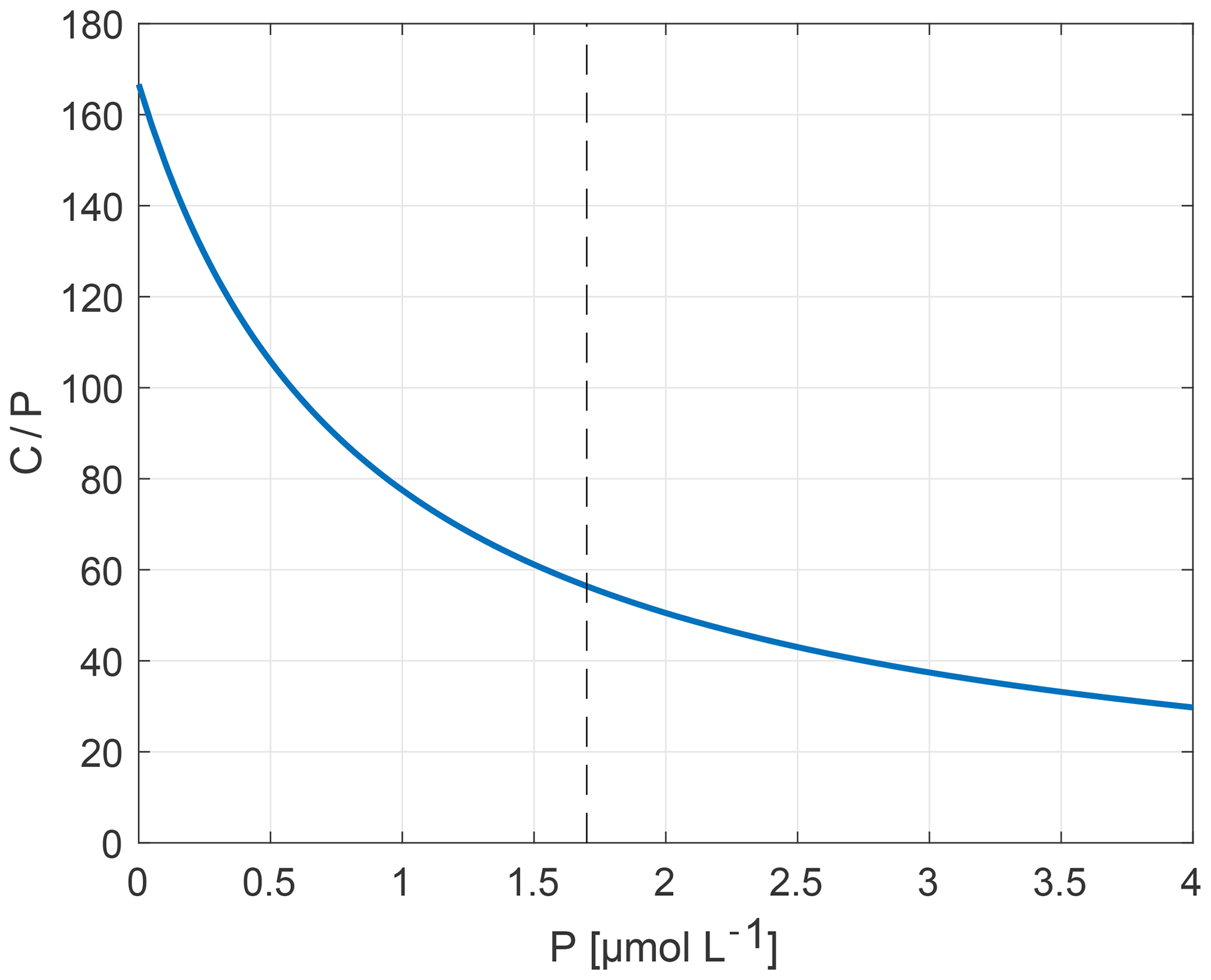
Figure 1Flexible stoichiometry C∕P (y axis) dependent on the P concentration (µmol L⁻¹) (x axis), as described by Eq. (1). Here, we extend the relationship beyond the observational interval 0–1.7 µmol L⁻¹ (bounded by dashed line) which forms the basis of the relation derived by Galbraith and Martiny (2015).

Download

2.3 Experiments

We start all experiments from an interglacial–modern (IG-M) control state, which has been run for 10 000 years to steady state, using either Redfield (Ctrl_RED) or variable (Ctrl_GAM) stoichiometry. The control states have a prescribed $p{\mathrm{CO}}_{\mathrm{2}}^{\mathrm{atm}}$ of 278 ppm and the same climate (Table 1). However due to the differences in C∕P, they have different ocean carbon inventories (Table S1 in the Supplement). In Ctrl_GAM, the export flux of organic matter (see Ridgwell et al., 2007) has a global average C∕P composition of 121∕1, and thus the global ocean carbon storage is larger than in Ctrl_RED. This also suggests that a perturbation, which increases ocean storage of P through the biological pump, could cause storage of 15 (i.e. 121–106) more carbon atoms in simulations using GAM compared to RED, simply because the average composition of the formed biological material is different. To distinguish between the role of the flexibility of the stoichiometry and the change in the mean composition of organic material, we add a control state with fixed stoichiometry where C∕P = 121∕1 (henceforth denoted Ctrl₁₂₁).

Table 1List of experiments. Ensemble member acronyms, short descriptions of what the simulation tests, and specifications of parameter settings for each ensemble member. The $p{\mathrm{CO}}_{\mathrm{2}}^{\mathrm{atm}}$ is either prescribed to pre-industrial level (PI) = 278 ppm or freely varying with changes in climate and ocean circulation. The radiative forcing is either coupled to the $p{\mathrm{CO}}_{\mathrm{2}}^{\mathrm{atm}}$ of the atmospheric chemistry module of the model or fixed at a value corresponding to $p{\mathrm{CO}}_{\mathrm{2}}^{\mathrm{atm}}=\mathrm{185}$ ppm. The zonal albedo profile is either representative of IG-M conditions or of the LGM. The wind stress is either IG-M or has an adjusted peak in wind stress at $\pm {\mathrm{50}}^{\circ }$ N. The IG-M remineralization length scale (RLS) is 590 m. If RLS is changed, it is multiplied by a factor (fr). Dust forcing is either IG-M or representative of LGM. Each experiment is conducted using model versions with C∕P fixed at 106∕1 (Redfield, 1963,  denoted RED), C∕P variable with surface ocean PO₄ concentration (Galbraith and Martiny, 2015, denoted GM15), and C∕P fixed at 121∕1 (denoted 121; see Sect. 2.3).

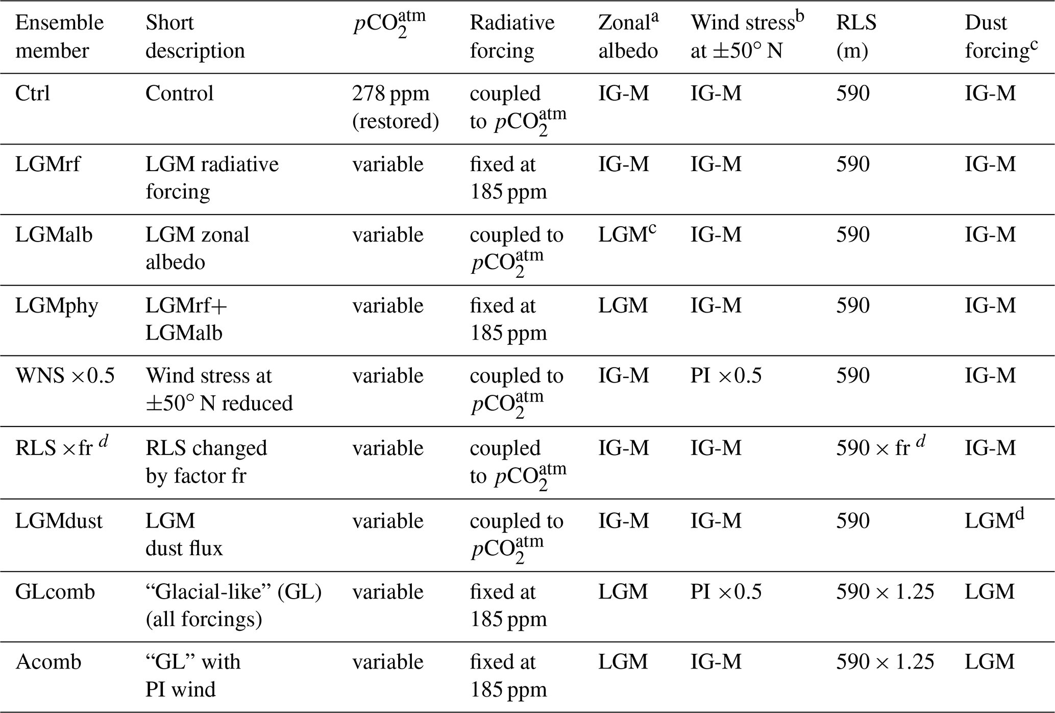
^a Calculated from the HADCM3 LGM (21 ka) simulation of Davies-Barnard et al. (2017). ^bSee Lauderdale et al. (2013) for example of reduced peak wind profile for the Southern Hemisphere. ^c Re-gridded LGM dust flux from Mahowald et al. (2006). ^d fr denotes multiplication factor for remineralization length scale. We test multiplication factors between 0.75 and 1.75, corresponding to a change in RLS between −25 % and +75 %.

Download Print Version | Download XLSX

In order to explore the effects of variable stoichiometry, we make a sensitivity study where we apply changes to boundary conditions, individually and in combination (see Sect. 2.3.3), that may be representative of changes that occurred during glacial periods. All experiments are listed in Table 1.

The applied changes in boundary conditions are

• physical perturbations (colder climate) of

  • –

    radiative forcing corresponding to LGM CO₂ = 185 ppm and

  • –

    zonal albedo profile representative of LGM (calculated from the LGM climate simulation of Davies-Barnard et al., 2017);

• physical perturbations (weaker overturning) of

  • –

    reduced wind forcing over the Southern Ocean (Lauderdale et al., 2013, e.g.) and north of 35^∘ N (see Sect. 2.3.1); and

• biological perturbations of

  • –

    changed remineralization length scale (e.g. Matsumoto, 2007; Chikamoto et al., 2012; Menviel et al., 2012) and

  • –

    increased dust forcing, as simulated for the LGM (regridded from Mahowald et al., 2006).

By applying the above perturbations, we aim to approach, but not fully resolve, some of the characteristics of the LGM ocean, which appears to have had a global average ocean temperature ($\stackrel{\mathrm{‾}}{T_{\mathrm{oce}}}$) 2.57 ±0.24 ^∘C colder than the Holocene (Bereiter et al., 2018), a weakly ventilated deep ocean (e.g. Menviel et al., 2017), and a more efficient biological pump (e.g. Sarmiento and Toggweiler, 1984; Martin, 1990; Sigman and Boyle, 2000). We also aim to increase carbon retention in the deep ocean (Muglia et al., 2018).

The physical perturbations serve to achieve a colder climate ($\stackrel{\mathrm{‾}}{T_{\mathrm{oce}}}$ cools by 2.1 ^∘C compared to Ctrl, thus 80 % of the observed 2.6 ^∘C; see Sect. 3.2.1) and weaker overturning (see Sect. 3.2.2 and Fig. 2) with a longer residence time of the Antarctic Bottom Water (AABW) cell compared to Ctrl. Colder conditions achieve a stronger solubility pump, thereby strengthening the retention of carbon in the deep ocean. As the physical perturbations affect the ocean circulation and temperature, they also affect the nutrient distribution and the rates of nutrient upwelling and biological growth (slower growth in colder water). They thereby affect the biological productivity (Ridgwell et al., 2007).

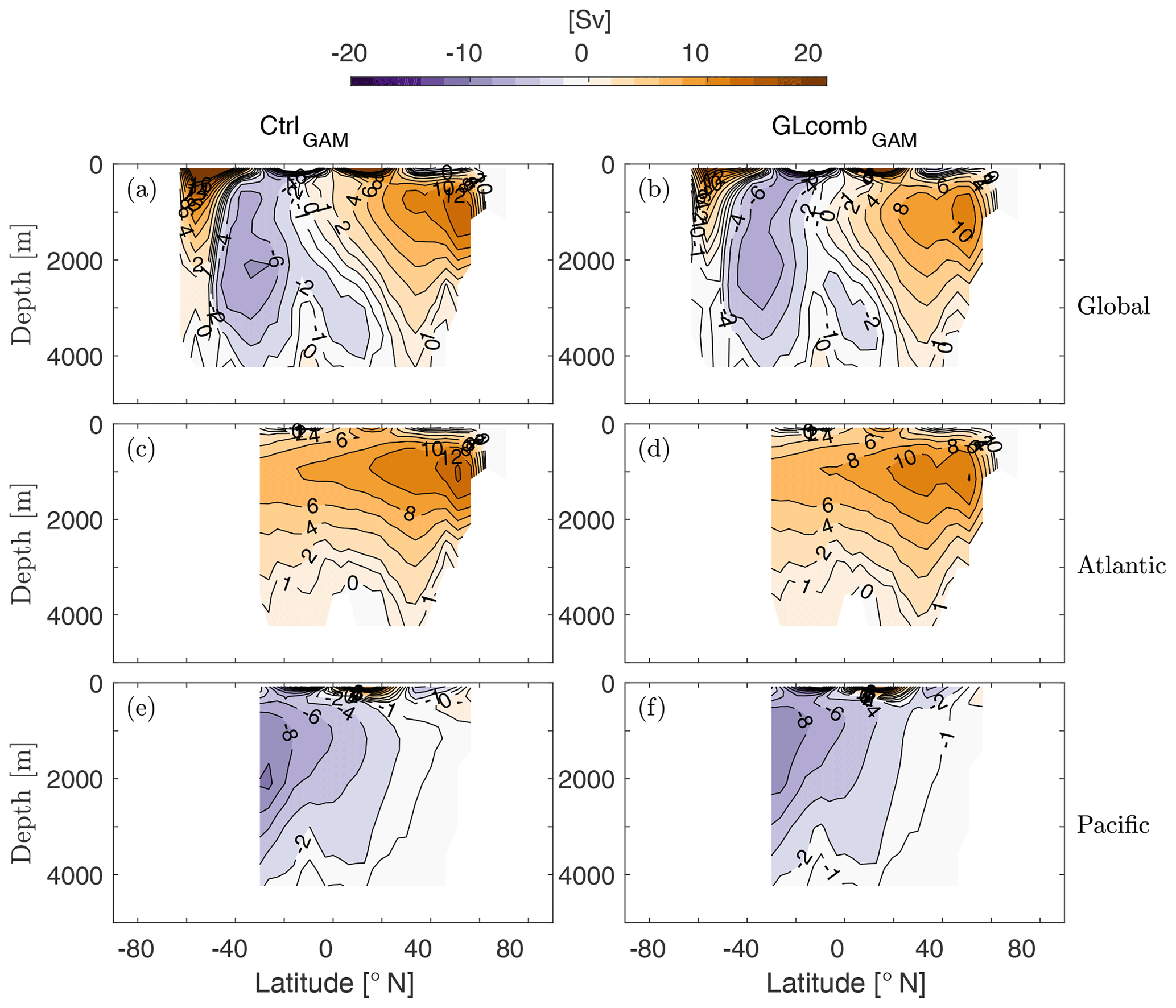
Figure 2The Eulerian component of the global (a, b), Atlantic (c, d), and Pacific (e, f) ocean meridional overturning stream function (1 Sv = 10⁶ m³ s⁻¹) of Ctrl_GAM (a, c, e) and GLcomb_GAM (b, d, f). Note that the eddy-induced transport of tracers is taken into account through a skew-diffusive flux (Griffies, 1998) that is present in the velocity fields used to compute the Eulerian stream function.

Download

The biological perturbations serve to achieve a more efficient biological pump, which is connected with increased retention of nutrients and carbon in the deep ocean, and lower surface nutrient concentrations in productive regions (see Sect. 3.2.3 and 3.2.4). With flexible stoichiometry, lower surface nutrient concentrations result in higher C∕P ratios, further increasing the export production and thereby the carbon retention in the deep ocean. In our experiments, we show that the flexible stoichiometry amplifies the response of the biological pump to both physical and biological perturbations.

The perturbations and the experiments are described in detail in Sect. 2.3.1–2.3.3.

2.3.1 Physical perturbations

We change the physical conditions for climate by changing radiative forcing and albedo to LGM-like conditions and denote these changes as LGMphy. We set the radiative forcing in the model to correspond to an atmosphere with 185 ppm CO₂ instead of 278. However, we allow the $p{\mathrm{CO}}_{\mathrm{2}}^{\mathrm{atm}}$ to freely evolve (starting from the value of 278 ppm of the Ctrl-state atmosphere) in response to the cooler climate. For albedo, we apply a zonal LGM albedo profile (calculated from the LGM climate simulation of Davies-Barnard et al., 2017). Assumptions of a simple zonal profile, instead of a 2D field re-gridded from PMIP LGM simulations, allow for a better consistency with the original zonal mean albedo profile developed for the modern configuration of GENIE (Marsh et al., 2011). Together, the changes in radiative forcing and albedo cause the global ocean average temperature ($\stackrel{\mathrm{‾}}{T_{\mathrm{oce}}}$) to decrease by 2.1 ^∘C compared to Ctrl (see Sect. 3.2.1).

To achieve a longer residence time of the AABW water mass, and an associated increase in carbon and nutrient retention, we apply weaker winds (denoted WNA ×0.5). We use the Southern Ocean wind profile of Lauderdale et al. (2013), where the peak westerly wind strength at 50°S has been halved compared to the control state (see Sect. 2.3.3). The winds north and south of the peak are reduced accordingly to give a continuous profile (see Fig. 2a of Lauderdale et al., 2013). The result is a weaker overturning (see Table 2) and a longer residence time of the AABW as may be expected for the glacial ocean (Menviel et al., 2017; Skinner et al., 2017) (see also Sect. 4.5). Thus, this approach is justifiable in a model of reduced complexity. However, there are studies suggesting that the Southern Ocean winds may in fact have been stronger during glacial times (Sime et al., 2013, 2016; Kohfeld et al., 2013). To avoid an expansion of the North Atlantic Deep Water (NADW) overturning cell that would be inconsistent with the glacial ocean (Duplessy et al., 1988; Lynch-Stieglitz et al., 1999; Curry and Oppo, 2005; Marchitto and Broecker, 2006; Hesse et al., 2011), winds north of 35^∘ N are also gradually reduced so that the wind strength north of 50^∘ N is reduced by half compared to the control state. In cGENIE, gas transfer velocities are calculated as a function of wind speed (described in Ridgwell et al., 2007), and following Wanninkhof (1992). Consequently, weaker winds also lead to reduced gas exchange with the atmosphere.

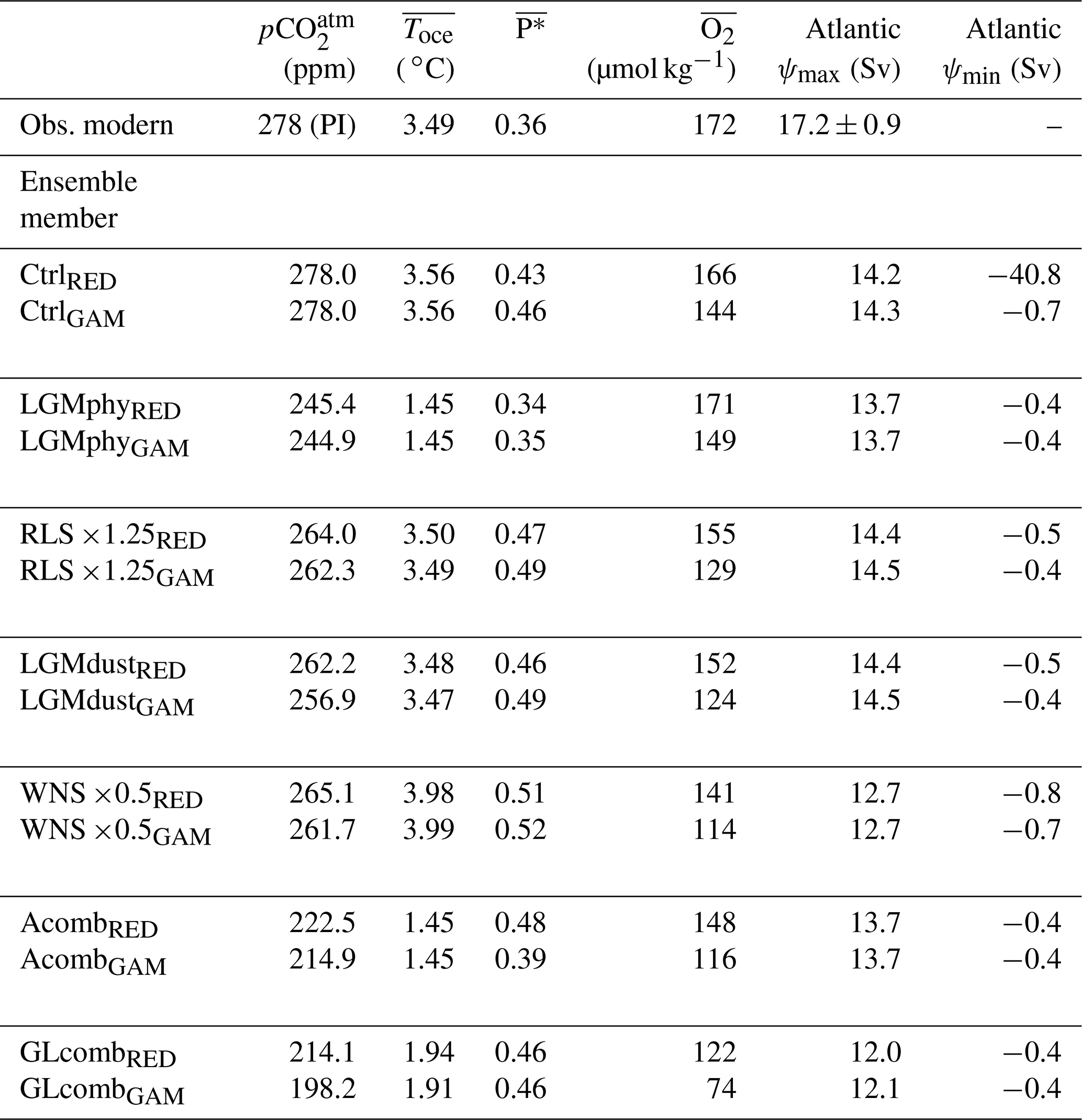
Table 2Atmospheric CO₂ ($p{\mathrm{CO}}_{\mathrm{2}}^{\mathrm{atm}}$, ppm); global ocean averages of temperature ($\stackrel{\mathrm{‾}}{T_{\mathrm{oce}}}$, ^∘C), $\stackrel{\mathrm{‾}}{{\mathrm{P}}^{*}}$, and $\stackrel{\mathrm{‾}}{{\mathrm{O}}_{\mathrm{2}}}$ (µmol kg⁻¹); Atlantic overturning stream function (ψ, sverdrups (Sv)); and maximum and minimum north of −30^∘ N, for observations, and for selected ensemble members in each model version (RED and GAM). Climatological modern-day $\stackrel{\mathrm{‾}}{T_{\mathrm{oce}}}$ and $\stackrel{\mathrm{‾}}{{\mathrm{O}}_{\mathrm{2}}}$ were computed using the World Ocean Atlas 2018 (Locarnini et al., 2018; Garcia et al., 2018c). $\stackrel{\mathrm{‾}}{{\mathrm{P}}^{*}}$ for the modern-day ocean is estimated by Ito and Follows (2005). Average modern-day AMOC strength is estimated by McCarthy et al. (2015) from the RAPID-MOCHA array at 26^∘ N (corresponding to Atlantic ψ_max in the model). Note that observed $p{\mathrm{CO}}_{\mathrm{2}}^{\mathrm{atm}}$ is given for pre-industrial (PI) climate, as we do not model anthropogenic release of CO₂.

Download Print Version | Download XLSX

2.4 Observations

For comparison and validation of model results, we use records of ocean-state variables from climatological mean fields of modern observations and proxy observations from the LGM.

Modern data of ocean temperature, oxygen, and nutrients are retrieved from the World Ocean Atlas 2018 (Locarnini et al., 2018; Garcia et al., 2018c, b) and we use the proxy estimates of LGM ocean temperature from Bereiter et al. (2018). Average modern-day strength of the Atlantic meridional overturning circulation (AMOC) is estimated by McCarthy et al. (2015) from the RAPID-MOCHA array at 26^∘ N.

We use model–data comparison of benthic δ¹³C to assess the statistical similarity (correlation) between both the model control state and glacial-like state (see Sect. 2.3) to benthic δ¹³C data representing the late Holocene (0–6 ka, HOL) and Last Glacial Maximum (19–23 ka, LGM) (Peterson et al., 2014). Locations of core sites can be seen in Fig. S1 in the Supplement (see also Fig. 1 in Peterson et al., 2014). Note that LGM benthic δ¹³C is more ¹³C-depleted than that in the Holocene due to the addition of ¹³C-depleted terrestrial carbon to the glacial ocean (Shackleton, 1977; Curry et al., 1988; Duplessy et al., 1988), which is not simulated in our model experiments. Therefore, to compare our glacial-like simulations (GLcomb) to LGM observations, we subtract a Holocene–LGM global average difference of 0.32 ‰ (Gebbie et al., 2015) from the GLcomb experiments. Gebbie et al. (2015) state that the wide range of error for the estimate of glacial-to-modern change in benthic δ¹³C of 0.32±0.20 ‰ suffers from a lack of observations in all ocean basins but the Atlantic. Therefore, we place more emphasis on the results of the model–data comparison in the Atlantic than in the Indo-Pacific sector.

2.5 Nutrient utilization efficiency

The extent to which biology succeeds in using the available nutrients can be determined by calculating the nutrient utilization efficiency $\stackrel{\mathrm{‾}}{{\mathrm{P}}^{*}}$ (Ito and Follows, 2005; Ödalen et al., 2018),

which is the fraction of remineralized (P_reg) to total (P_tot) nutrients (in this case, PO₄) in the ocean. Overlines denote global averages. Remineralized nutrients have been transported from the surface to the interior ocean by the biological pump, and P_rem is given by

Here, P_pre is preformed PO₄ – the concentration of PO₄ that was present in the water parcel as it sank, and thus the fraction that was not used by biology in the surface ocean. In cGENIE, the concentration of preformed tracers is set in the surface ocean and then passively advected through the ocean interior (Ödalen et al., 2018). The biological pump also captures carbon, and a similar relationship can be used for concentrations of DIC, where

DIC_rem is used to compute the ocean storage of remineralized acidic carbon (AC_rem; see Appendix A). AC_rem is biological carbon that entered the ocean in the form of CO₂ in soft tissue (as opposed to carbonates in hard tissue), measured independently of oxygen consumption and/or remineralized phosphate.

In cGENIE, P_pre and DIC_pre are modelled as passive tracers (Ödalen et al., 2018). Hence, we can use the model output for P_pre in Eq. (3) to compute $\stackrel{\mathrm{‾}}{{\mathrm{P}}^{*}}$ (Eq. 2).

In a model with a fixed Redfield ratio, $\stackrel{\mathrm{‾}}{{\mathrm{P}}^{*}}$ determines the effect of the biological pump on $p{\mathrm{CO}}_{\mathrm{2}}^{\mathrm{atm}}$. For example, it has been found that a higher $\stackrel{\mathrm{‾}}{{\mathrm{P}}^{*}}$ in the initial state gives a lower potential for drawdown of $p{\mathrm{CO}}_{\mathrm{2}}^{\mathrm{atm}}$ in response to similar perturbations (Marinov et al., 2008; Ödalen et al., 2018). However, with variable stoichiometry this is no longer true, since the amount of carbon retained in the deep ocean is not necessarily proportional to $\stackrel{\mathrm{‾}}{{\mathrm{P}}^{*}}$.

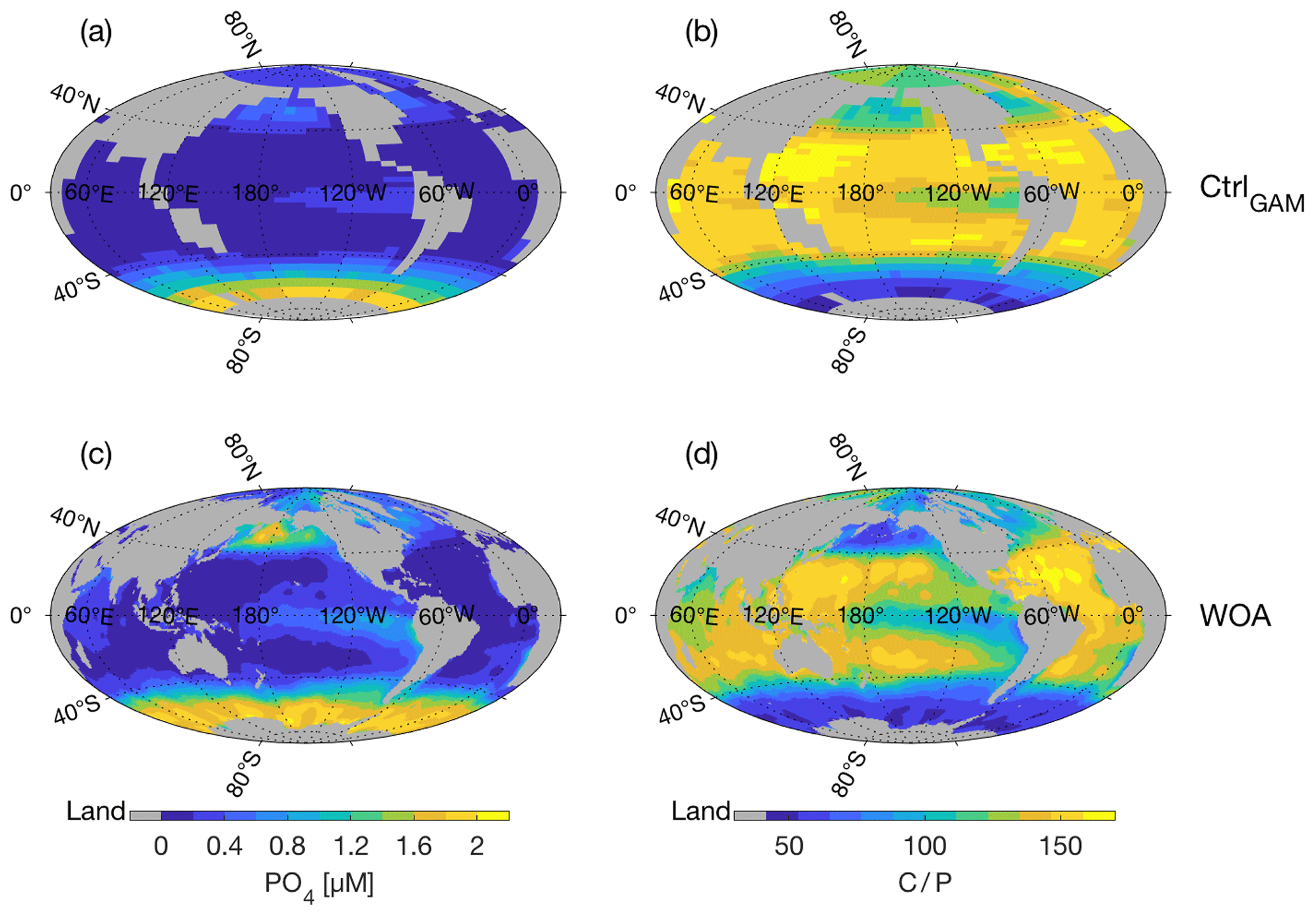
Figure 3Surface PO₄ concentration (µM) (a, c) and corresponding C∕P as calculated using parametrization of Galbraith and Martiny (2015) (b, d). Panels show Ctrl_GAM (a, b) and climatological mean fields (World Ocean Atlas 2018, Garcia et al., 2018b) (c, d).

3.1 Control states

3.1.3 Ocean dissolved O₂

The most apparent difference between Ctrl_RED and Ctrl_GAM is in deep-ocean oxygen concentrations, where the global ocean average dissolved O₂ concentration ($\stackrel{\mathrm{‾}}{{\mathrm{O}}_{\mathrm{2}}}$) in Ctrl_GAM (144 µmol kg⁻¹) is lower than in Ctrl_RED and Ctrl₁₂₁ (166 and 152 µmol kg⁻¹ respectively). Compared to climatological mean fields (World Ocean Atlas 2018, Fig. 4a–b), both Ctrl_RED (Fig. 4c–d) and Ctrl_GAM (Fig. 4e–f) agree reasonably well with the real ocean. Ctrl_GAM appears to better capture the equatorial oxygen minimum in the Atlantic basin than Ctrl_RED but is too low in the North Pacific. In Ctrl_GAM (Fig. 4f), the North Pacific is markedly lower in oxygen than in Ctrl_RED (Fig. 4d) and even anoxic in the oxygen minimum zone (OMZ). This should be kept in mind when analysing the oxygen sections of the glacial-like states GLcomb_RED (Fig. 4g–h) and GLcomb_GAM (Fig. 4i–j). Global averages for dissolved O₂ are given in Table 2.

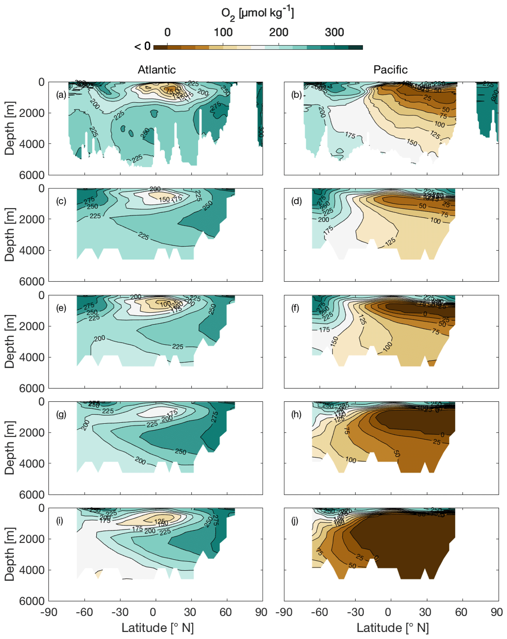
Figure 4Sections of O₂ concentration (µmol kg⁻¹) along 25^∘ W in the Atlantic basin (left-hand column) and along 135^∘ W in the Pacific basin (right-hand column). Panels show climatological mean fields (World Ocean Atlas 2018, Garcia et al., 2018c) (a, b) and model states Ctrl_RED (c, d), Ctrl_GAM (e, f), GLcomb_RED (g, h), and GLcomb_GAM (i, j).

Download

3.1.4 Ocean δ¹³C

By comparing Ctrl_RED δ¹³C and Holocene (0–6 ka, HOL) benthic δ¹³C values, we estimate a global model–data correlation of 0.78 (Table S3). The modern-day Atlantic Ocean has a distinctive spatial δ¹³C pattern (Figs. 5a, S1) with ¹³C-enriched values in the intermediate-depth (<2 km) North Atlantic and Nordic Seas and ¹³C-depleted values in the deep (>2.5 km) South Atlantic. While the model produces a weaker gradient than the observed HOL Atlantic Ocean (corr. 0.50, Table S3) the model correlates well with eastern Atlantic δ¹³C records (Fig. S1). For the Indo-Pacific, the weaker benthic δ¹³C gradient is well represented by the model (Fig. 5e). This pattern emerges mainly due to ¹³C-depleted, biologically sourced carbon that is accumulated in the weak circulation region of the interior North Pacific (Matsumoto et al., 2002). However, Indo-Pacific δ¹³C values of Ctrl_RED are overall lower than the HOL observations. The overall model–data correlation for the Indo-Pacific is 0.39 (Table S3). Comparing the control states of the RED and GAM model versions, δ¹³C patterns (Figs. 5a, e and S3a, e) and model–data correlations with HOL observations (Table S3) are similar between the model versions, with somewhat lower correlations for GAM.

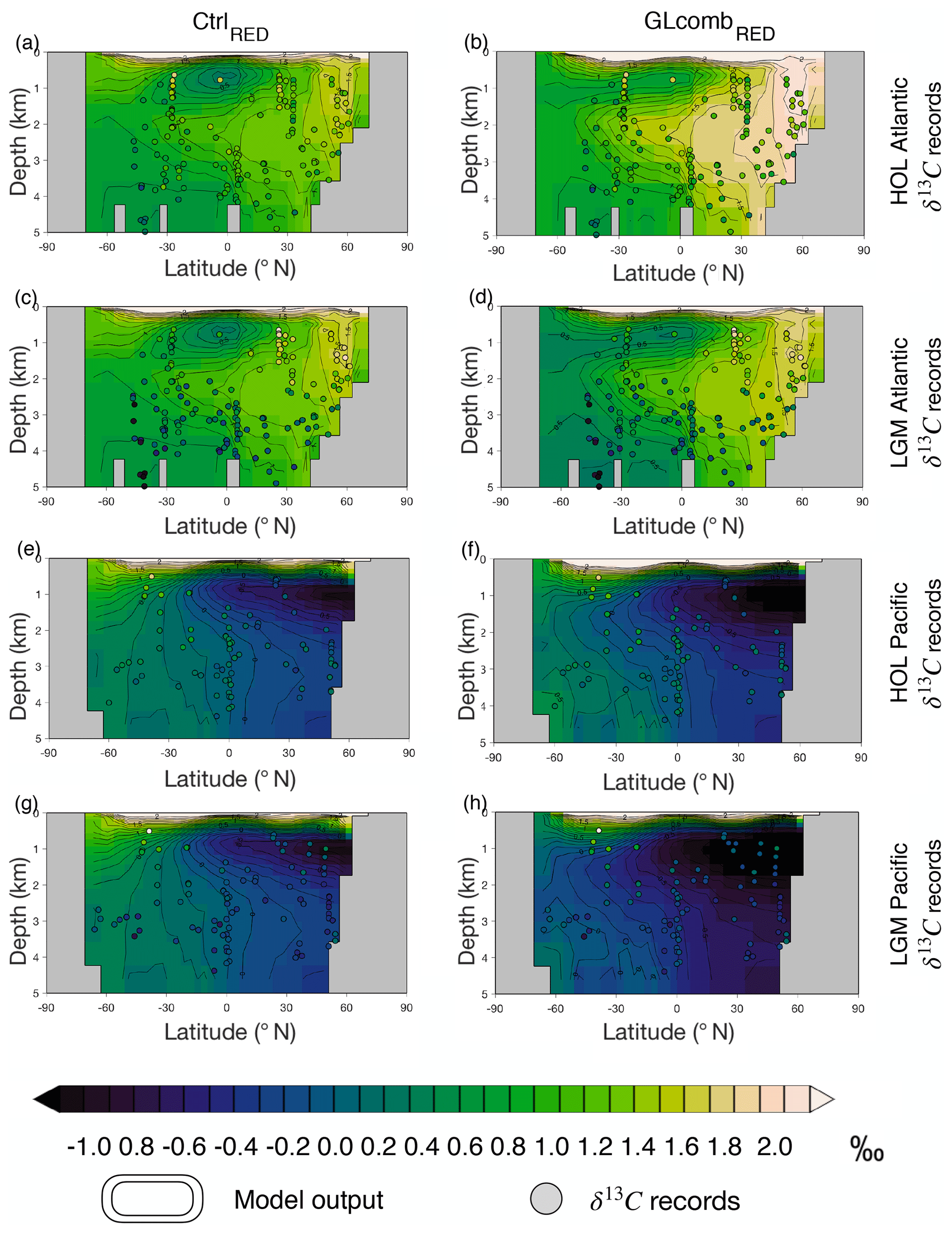
Figure 5Model ocean δ¹³C (contours) compared to the two proxy record time slices (HOL and LGM) of benthic δ¹³C (circles) of Peterson et al. (2014). The upper half of the figure shows the Atlantic Ocean (a–d), while the lower half shows the Pacific Ocean (e–h). The columns represent the model simulations (Ctrl_RED or Ctrl_GAM), while each row represents one of the proxy record time slices (HOL or LGM). The left-hand column shows Ctrl_RED (a, c, e, g) and the right-hand column shows GLcomb_RED (b, d, f, h). The rows show, from top to bottom, (a, b) HOL Atlantic, (c, d) LGM Atlantic, (e, f) HOL Pacific, and (g, h) LGM Pacific. Note that, before we compare GLcomb_RED to LGM observations (d, h), a constant of 0.32 ‰ is subtracted from the simulated δ¹³C, to account for terrestrial release of δ¹³C-depleted terrestrial carbon which is not modelled. The corresponding comparison for model version GAM is shown in Fig. S3.

Download

3.2 Sensitivity experiments

The applied changes listed in Table 1 cause changes in ocean characteristics such as overturning circulation, temperature, surface nutrient distributions, and biological productivity, which result in changed $p{\mathrm{CO}}_{\mathrm{2}}^{\mathrm{atm}}$. The resulting steady-state global average values for temperature ($\stackrel{\mathrm{‾}}{T_{\mathrm{oce}}}$), dissolved oxygen ($\stackrel{\mathrm{‾}}{{\mathrm{O}}_{\mathrm{2}}}$), and nutrient utilization efficiency $\stackrel{\mathrm{‾}}{{\mathrm{P}}^{*}}$, as well as the maximum and minimum of the Atlantic meridional overturning stream function, are listed in Table 2.

3.2.1 Radiative forcing and albedo

In the simulations where radiative forcing and albedo are changed to represent LGM conditions (LGMrf + LGMalb = LGMphy), the reductions in $p{\mathrm{CO}}_{\mathrm{2}}^{\mathrm{atm}}$ are similar in the RED and the GAM model versions. In LGMphy, the resulting $p{\mathrm{CO}}_{\mathrm{2}}^{\mathrm{atm}}$ is 245.4 and 244.9 ppm, thus showing a reduction of 33 ppm compared to the Ctrl 278 ppm (Fig. 6). Here, variable C∕P does not impact the results, because changes in the surface nutrient distribution (Fig. 7a), and the associated changes in C∕P (Fig. 8a), are limited to very high latitudes where productivity is already low in the control state, due to low temperatures and a lack of light and iron. The drawdown of $p{\mathrm{CO}}_{\mathrm{2}}^{\mathrm{atm}}$ can mainly be attributed to the increase in solubility carbon (C_sat,T), due to ocean cooling, and to an increase in sea ice, which prevents air–sea gas exchange and therefore causes an increase in disequilibrium carbon (C_dis) (Ödalen et al., 2018). Ocean cooling amounts to 2.1 ^∘C in LGMphy compared to Ctrl ($\stackrel{\mathrm{‾}}{T_{\mathrm{oce}}}$ in Table 2). In cGENIE, the increase in C_sat,T associated with ocean cooling corresponds to $\sim \mathrm{7}\pm \mathrm{1.5}$ ppm ^∘C⁻¹ (Ödalen et al., 2018, Supplement Fig. S1). Thus, in LGMphy C_sat,T and C_dis should contribute roughly 40 % and 60 % respectively of the change in $p{\mathrm{CO}}_{\mathrm{2}}^{\mathrm{atm}}$. Note that cGENIE underestimates the true effect of ocean cooling on solubility, due to a temperature restriction on the solubility constants (Ödalen et al., 2018). This temperature restriction limits solubility from changing below 2.0 ^∘C. In this case, the solubility effect on $p{\mathrm{CO}}_{\mathrm{2}}^{\mathrm{atm}}$ of reducing $\stackrel{\mathrm{‾}}{T_{\mathrm{oce}}}$ by 2.1 ^∘C (from 3.6 to 1.5 ^∘C, ∼15 ppm) is thus comparable to only 1.6 ^∘C of cooling (from 3.6 to 2.0 ^∘C, ∼11 ppm), and the solubility effect is underestimated by ∼4 ppm. As we do not change salinity, we are simultaneously likely to overestimate the increase in solubility between Ctrl and a glacial-like state by ∼6 ppm (Kohfeld and Ridgwell, 2009). This effect is consistent for any choice of C∕P parametrization and is therefore not explored further.

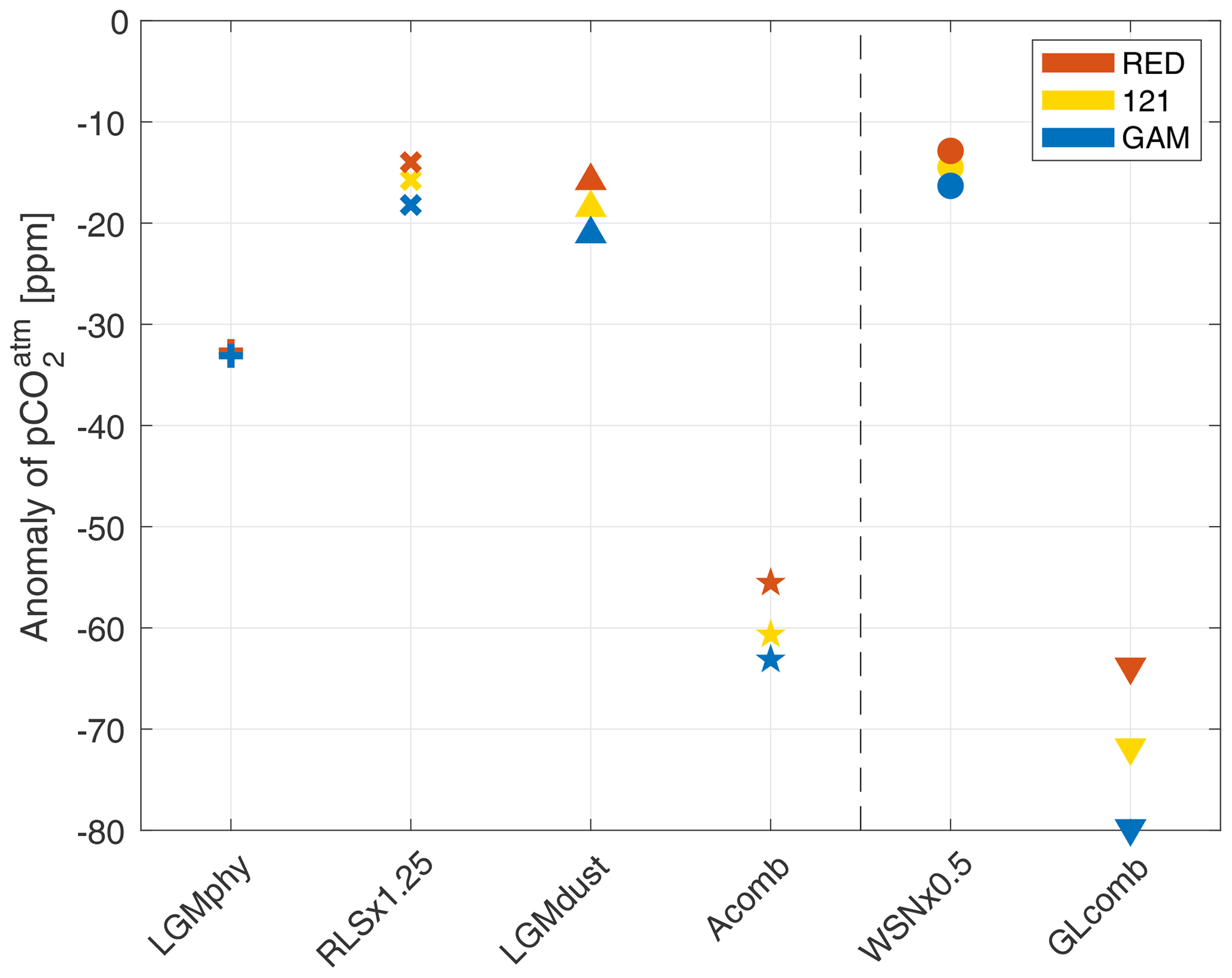
Figure 6Resulting CO₂ anomaly, with respect to the control-state 278 ppm, of the sensitivity experiments LGMphy (plus symbol), RLS ×1.25 (times symbol), LGMdust (upward arrowheads), and WSN ×0.5 (circles) and of the combined experiments Acomb (stars) and GLcomb (downward arrowheads). Results of the different model versions RED, 121, and GAM are shown in red, yellow, and blue respectively. The vertical dashed line separates simulations without (left) and with (right) wind perturbation.

Download

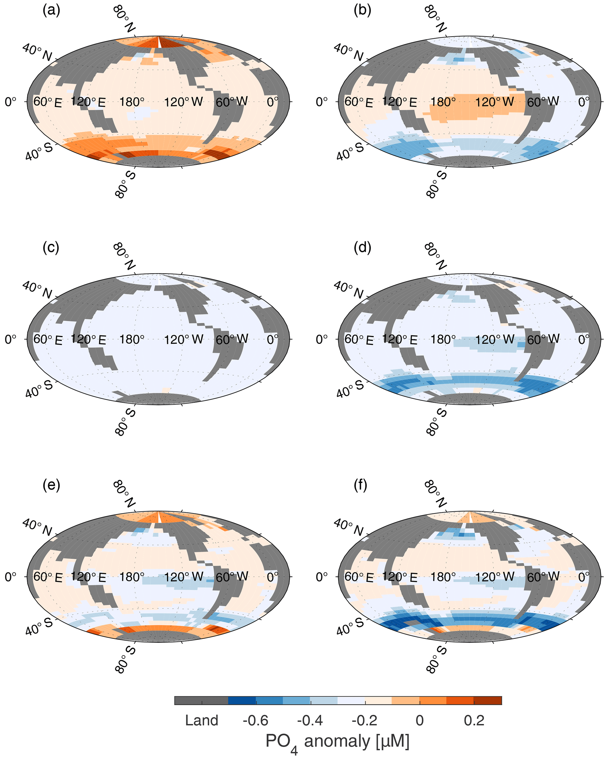
Figure 7Surface PO₄ anomaly (µM), with respect to surface concentration of PO₄ in Ctrl_GAM (Fig. 3a), for (a) LGMphy_GAM, (b) WSN ×0.5_GAM (c) RLS ×1.25_GAM, (d) LGMdust_GAM, (e) Acomb_GAM, and (f) GLcomb_GAM. Changes in surface nutrient fields are similar for all three model versions (RED, GAM, 121); thus only GAM is shown.

3.2.2 Reduced wind forcing

When the peak of Southern Ocean (henceforth SO) winds is reduced, the strength of the overturning circulation of AABW decreases (see difference in Southern Hemisphere overturning stream function between Fig. 2a and b). Thus, given that the volume of AABW does not change, its residence time increases. This also means that the upwelling nutrient-rich water in the SO stays near the surface for longer and loses more nutrients before being subducted. This decreases the SO concentration of preformed phosphate in WNS ×0.5_RED compared to Ctrl, as seen in Fig. 7b, and increases the nutrient utilization efficiency $\stackrel{\mathrm{‾}}{{\mathrm{P}}^{*}}$ (Table 2, Fig. 9). This leads to a drawdown of $p{\mathrm{CO}}_{\mathrm{2}}^{\mathrm{atm}}$ of 12.9 ppm compared to Ctrl_RED (Fig. 6). As the nutrient concentration in the SO decreases (Fig. 7b), the flexible C∕P ratio (Fig. 8b) leads to an increased carbon capture efficiency in GAM compared to RED (see GLcomb-Ctrl of biologically sourced carbon (AC_rem) in Fig. 9), which is partly compensated for by a reverse effect in the Pacific equatorial region. Consequently, in WSN×0.5_GAM, we get a reduction of $p{\mathrm{CO}}_{\mathrm{2}}^{\mathrm{atm}}$ of 16.3 ppm compared to Ctrl_GAM (Fig. 6). Hence, for halved peak wind stress at ±50^∘ N, the flexible stoichiometry increases the drawdown by ∼26 %.

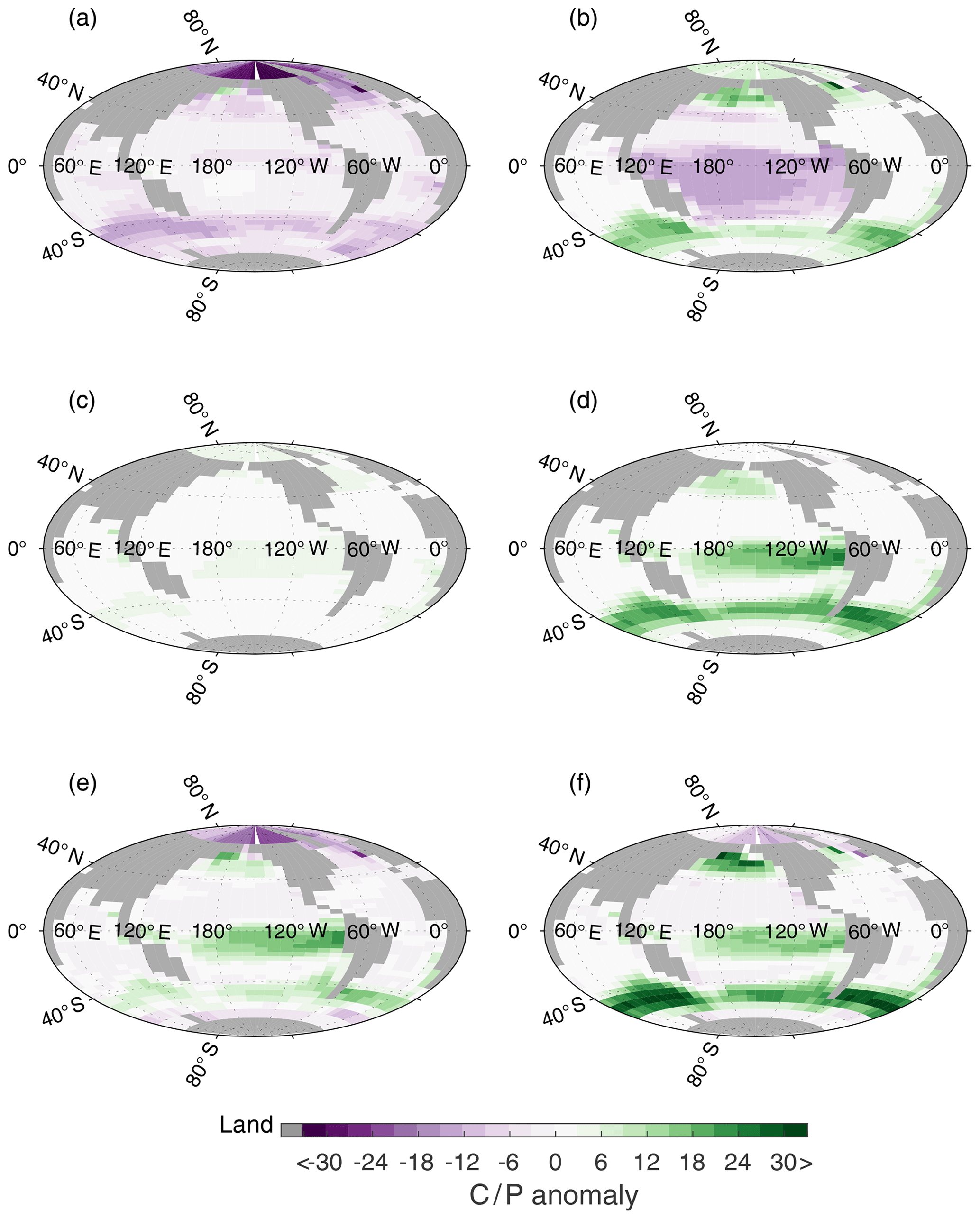
Figure 8Surface C∕P anomaly, with respect to C∕P of Ctrl_GAM (Fig. 3b), for (a) LGMphy_GAM, (b) WSN ×0.5_GAM (c) RLS ×1.25_GAM, (d) LGMdust_GAM, (e) Acomb_GAM, and (f) GLcomb_GAM.

Figure 9Remineralized acidic carbon (AC${}_{\mathrm{rem}}={\mathrm{DIC}}_{\mathrm{rem}}-(\mathrm{1}/\mathrm{2})\times {\mathrm{ALK}}_{\mathrm{rem}}$; see Appendix A) as a function of $\stackrel{\mathrm{‾}}{{\mathrm{P}}^{*}}$. Simulations using model versions RED and GAM are shown in red and blue respectively. Different symbols indicate the sensitivity experiments, listed in the panel on the right-hand side. Red and blue lines show linear least-squares fits to the separate ensembles for RED and GAM. Panels illustrate (a) the deviation from the least-squares fit of the GAM ensemble as opposed to the RED ensemble, (b) the linear fits extrapolated to the origin, and (c) a zoom-in around the origin, where the RED (red) line goes through the origin, while the GAM (blue) does not.

Download

3.3 Combined experiments

We show the results of two different combined simulations; Acomb and GLcomb. GLcomb is the “glacial-like” simulation, which combines all the sensitivity experiments (Table 1). Acomb omits the reduction in wind stress.

4.1 Accounting for variable C∕P in ocean carbon cycle models

The representation of ocean biology in general circulation models (GCMs) tends to be oversimplified (Le Quéré et al., 2005) and the development of the models is often held back by constraints imposed by maintaining the computational efficiency of the model. The Galbraith and Martiny (2015) empirical model is simple and based on nutrient variables that are already present in biogeochemical models (nitrate and phosphate). By implementing the GAM parametrization, or possibly a power law such as that described by Tanioka and Matsumoto (2017), an additional facet of the complexity of ocean biology can be implicitly accounted for at a relatively small computational cost. Previous model ensemble studies have shown that this type of dynamical response of the biology to changes in the modelled ocean state can improve the model's ability to realistically simulate ocean biogeochemistry (Buchanan et al., 2018). In pre-industrial and future simulations respectively, Buchanan et al. (2018) and Tanioka and Matsumoto (2017) find that the flexible stoichiometry acts to stabilize the response of ocean DIC to changes in the physical (circulation) state. In our glacial-like simulations, we find that the response of ocean DIC, and thus $p{\mathrm{CO}}_{\mathrm{2}}^{\mathrm{atm}}$, to the combined perturbations is greater in the simulations with flexible stoichiometry. Nonetheless, our study confirms the potential importance of dynamical biological response for the outcome of model studies.

The approach taken by both Galbraith and Martiny (2015) and Tanioka and Matsumoto (2017) is to adapt a function to species-independent C : P observations. This means that they account for the adaptation of plankton to the surrounding conditions, in terms of both species composition and individuals being more frugal in low-nutrient conditions. This is one of the main advantages of such an approach, as it can be applied in a model without different plankton functional types, which is what we use here. Ganopolski and Brovkin (2017) appear to succeed with full glacial–interglacial CO₂ cycles in CLIMBER-2, which does not have flexible stoichiometry for primary producers but which has a temperature limitation on growth and explicit phyto- and zooplankton with different C uptake rates. This combination may perhaps achieve a similar response in carbon export in their simulations, when moving into a colder climate, as the flexible stoichiometry does in our simulations. The next step to approach a more realistic modelling of the biological pump would be to include a representation of preferential remineralization of nutrients (e.g. Kolowith et al., 2001; Letscher and Moore, 2015), but this goes beyond the scope of the present study.

One drawback of the Galbraith and Martiny (2015) approach is that it assumes that the C∕P ratio continues to increase continuously with increasing [PO₄]. As such, in a high-surface-[PO₄] region like the Southern Ocean, GAM does not represent the effects on C∕P of temperature and light and the associated non-linear effects that could be of importance here (e.g. Yvon-Durocher et al., 2015; Tanioka and Matsumoto, 2017; Moreno et al., 2018). Up to [PO₄]=1.7 µM, the GAM parametrization fits the binned observational data well (see Figs. 1 and S2 in Galbraith and Martiny, 2015). To account for the lack of observational data at higher [PO₄] in Galbraith and Martiny (2015), we have tested the effect of saturation of the C∕P ratio at higher [PO₄] in Ctrl and GLcomb simulations where we kept $\mathrm{C}/\mathrm{P}=\mathrm{55}/\mathrm{1}$ at [PO₄]>1.7 µM. The increase in ocean carbon storage and decrease in $p{\mathrm{CO}}_{\mathrm{2}}^{\mathrm{atm}}$ between Ctrl and GLcomb are nearly identical with GAM; thus saturation of the C∕P ratio at very high [PO₄] causes no noticeable impact on our results.

Our sensitivity experiments RLS ×0.75 and RLS ×1.25 reveal that the response in $p{\mathrm{CO}}_{\mathrm{2}}^{\mathrm{atm}}$ to the perturbation is enhanced in GAM compared to RED for both increased and decreased RLS. While increased RLS would be an effect of ocean cooling, and thus of interest for glacial studies, reduced RLS would be a consequence of ocean warming (Matsumoto, 2007). Matsumoto (2007) describes how decreased RLS would have a positive feedback on $p{\mathrm{CO}}_{\mathrm{2}}^{\mathrm{atm}}$ in a future warming climate. Our results imply that flexible C∕P could have a further reinforcing effect on this feedback. It would therefore be of interest to apply a parametrization of flexible C∕P in models used for simulations of future climate feedbacks.

4.2 Decoupling of biologically sourced carbon and nutrient utilization efficiency

Many studies have suggested increased ocean storage of organic carbon as a potentially important contributor to the low glacial $p{\mathrm{CO}}_{\mathrm{2}}^{\mathrm{atm}}$ (e.g. Sarmiento and Toggweiler, 1984; Martin, 1990; Archer et al., 2000; Sigman and Boyle, 2000). However, biological production depends on water temperature (Eppley, 1972) and decreases in cold conditions. This temperature effect is parameterized in cGENIE as a local temperature-dependent uptake rate modifier proportional to $e^{(T/\mathrm{15.9}{}^{\circ }\mathrm{C})}$, and we see overall reduced productivity in our cold climate simulations (see e.g. LGM_phy, Table S1). As the climate cools, the temperature effect leads to a decrease in biological productivity and a subsequent decrease in $\stackrel{\mathrm{‾}}{{\mathrm{P}}^{*}}$ (see LGM_phy in Fig. 9). If productivity decreases, other mechanisms are needed to offset this decrease, if the total ocean storage of organic carbon is to increase. Mechanisms that can contribute to increased deep-ocean carbon retention are for example reduced SO overturning circulation (increased residence time of the AABW; Menviel et al., 2017) and deeper remineralization (Matsumoto, 2007; Chikamoto et al., 2012), which we apply through our perturbations in winds (Sect. 3.2.2) and RLS (Sect. 3.2.3). From our results, it is evident that variable stoichiometry can be another contributing factor. In our simulations, global average export production decreases, in terms of both POP (particulate organic phosphorus) and POC (particulate organic carbon), by 15 % between Ctrl_RED and GLcomb_RED because of the colder climate. However, the variable stoichiometry in GAM partly offsets this decrease in biological carbon capture – while the export production in terms of POP decreases by 17 %, the corresponding decrease in POC is only 10 %. Thus, in GLcomb_GAM we achieve an increase in ocean inventory of remineralized carbon, which exceeds the one of GLcomb_RED (Fig. 9).

Due to the competing effects between decreased export production and increased retention that are introduced by the different forcing components, the net change in P_rem, and thus in $\stackrel{\mathrm{‾}}{{\mathrm{P}}^{*}}$, is very small when moving from the control state (Ctrl) to the glacial-like state (GLcomb) (Fig. 9). In the fixed stoichiometry case (RED), there is a small net increase in $\stackrel{\mathrm{‾}}{{\mathrm{P}}^{*}}$ of 0.020 in GLcomb compared to Ctrl, which is linearly related to a small increase in storage of AC_rem in the ocean. In the case with variable stoichiometry (GAM), there is instead a very small decrease in $\stackrel{\mathrm{‾}}{{\mathrm{P}}^{*}}$ of 0.003. With a linear response, we would thus expect a decrease in storage of AC_rem as well. Instead, we see a reasonably large increase in global average AC_rem. In summary, we suggest this is a result of changes in surface P fields (see Fig. 7).

The reduced $p{\mathrm{CO}}_{\mathrm{2}}^{\mathrm{atm}}$ in GLcomb_GAM, compared to GLcomb_RED, can be explained by the non-linearity introduced by the local variability in C∕P. When changes in ocean circulation, remineralization depth, and dust deposition cause the local nutrient availability in the surface waters to change, this affects the elemental composition of the exported organic material (Fig. S5). In GLcomb, there is a reduction of the surface layer P concentration compared to Ctrl in some key (HNLC) regions. In GAM, this decrease in surface P results in an increase in C∕P. This further strengthens the biological pump in these key regions, resulting in a non-linear relationship between storage of remineralized phosphate and biologically sourced carbon (Fig. 9). In Ctrl_GAM, the average elemental C∕P composition is 121∕1. In GLcomb_GAM, this average is 134∕1 (Table S1, Fig. S5). This means that even though the same amount of P is exported to the deep ocean, the organic molecules carry more carbon, which is released in the deep ocean during remineralization. In Ctrl_GAM, the global average concentration of P_rem is 1.16 µmol kg⁻¹ (compared with 1.17 µmol kg⁻¹ in GLcomb_GAM). By increasing the average C∕P composition of 1.16 µmol kg⁻¹ organic molecules from 121 to 134 (i.e. by 13 units), this causes an increase in C_soft by ∼15 µmol kg⁻¹, which corresponds to the observed increase in AC_rem. From this, we conclude that, in a system where stoichiometry is variable on a local scale, ocean storage of biologically sourced CO₂ can change while the amount of remineralized nutrients remains constant.

Note also that Ctrl_GAM has a larger inventory of DIC as well as C_soft compared to Ctrl_RED. Ödalen et al. (2018) found that drawdown of $p{\mathrm{CO}}_{\mathrm{2}}^{\mathrm{atm}}$ in response to a perturbation is larger when the control state has a smaller inventory of DIC and C_soft. Yet, the effect of applying the same perturbation results in a larger drawdown of $p{\mathrm{CO}}_{\mathrm{2}}^{\mathrm{atm}}$ in GAM than in RED. This is opposite of the conclusions of Ödalen et al. (2018). The reason is that the flexible stoichiometry in effect increases the drawdown potential, which more than compensates for the increased carbon inventory in the control state. In GLcomb_GAM, the C∕P in global average export production increases from the control 121∕1 to 134∕1, which reflects the increased storage of organic carbon allowed by the flexible stoichiometry.

4.3 Implications of flexible C∕P for deep-ocean oxygen

Studies have shown that deep-ocean O₂ concentrations were lower during the LGM than in the Holocene (e.g. Bradtmiller et al., 2010; Jaccard and Galbraith, 2012; Galbraith and Jaccard, 2015). Here, we discuss implications of using flexible C∕P for the model's ability to reproduce ocean oxygen patterns and concentrations in the different time periods.

In the Atlantic, Ctrl_GAM (Fig. 4e) reproduces the climatological mean extent of the oxygen minimum zone (OMZ) (Fig. 4a) better than Ctrl_RED (Fig. 4c) does. In the Pacific Ocean, the O₂ gradient in the climatological mean fields (Fig. 4b) is more gradual compared to that of the control states (Fig. 4d, f), but the core of the OMZ is well reproduced by the model. The forcings applied to GLcomb are not sufficient to reproduce a full glacial state. Still, we do get a vertical expansion of the OMZ in GLcomb_RED (Fig. 4h) compared to Ctrl_RED (Fig. 4c), in agreement with the findings of Hoogakker et al. (2018). In GLcomb_GAM, oxygen depletion is too extensive (see below), but the tendency of vertical expansion compared to the control state is present here as well.

In our glacial-like states, we see a significant reduction of O₂ compared to the control state in both RED and GAM (Fig. 4d and e). This response is expected when we apply increased dust deposition and deeper remineralization (Galbraith and Jaccard, 2015), and the direction of the overall response of deep-ocean O₂ to the glacial-like forcings is in line with observations. The reduction in O₂ is stronger in GAM, due to the larger storage of respired carbon in this model version.

Finally, it should be noted that Ctrl_GAM (Fig. 4c) displays deeper oxygen minima in the oxygen minimum zones of both the Atlantic equatorial region and the North Pacific compared to what is seen in Ctrl_RED (Fig. 4b) and in climatological mean fields. In Ctrl_GAM, a large part of the interior North Pacific is anoxic (Fig. 4c), while the climatological mean fields (Fig. 4a) indicate very low oxygen levels, but not anoxia. As illustrated by simulations in Galbraith and de Lavergne (2018), variable stoichiometry in itself is not always sufficient to achieve widespread deep-ocean de-oxygenation in a model under glacial-like climate change. Among other factors, model ocean oxygen conditions are also dependent on deep water formation characteristics of the model (Galbraith and de Lavergne, 2018). The deep water formation characteristics of a model affect the amount of time available for remineralization and, consequently, the oxygen consumption. In addition, due to a lack of resolution deep water formation in climate models generally happens as open water convection, rather than as dense plumes along slopes (Heuzé et al., 2013). This may cause too much oxygen to be entrained into the deep ocean (Galbraith and de Lavergne, 2018). In cGENIE, this effect is small enough not to cancel the increased O₂ consumption caused by the higher average C∕P in Ctrl_GAM compared to Ctrl_RED.

In summary, the GAM version of the model quantitatively reproduces the observed O₂ patterns of both the LGM and the Holocene, but with too low concentrations. If this parametrization of variable stoichiometry is to be used in cGENIE in future studies, we suggest some retuning, for example by reducing the global average concentration of nutrients, to improve the representation of observed modern-day ocean O₂ concentrations in the GAM control state.

4.4 Effect of modified but fixed C∕P

Part of the observed difference in $p{\mathrm{CO}}_{\mathrm{2}}^{\mathrm{atm}}$ between GLcomb_RED and GLcomb_GAM results from a difference in global average C∕P in the control states (Ctrl_RED and Ctrl_GAM). In Ctrl_GAM, the average C∕P in the export production is close to 121∕1, instead of 106∕1 as in Ctrl_RED. We illustrate the consequences of this difference by running parallel simulations with fixed C∕P of 121∕1 (model version 121).

In a simulation with reduced wind stress (WNS ×0.5₁₂₁), $p{\mathrm{CO}}_{\mathrm{2}}^{\mathrm{atm}}$ is reduced by −14.5 ppm compared to Ctrl_RED (Table S2). The corresponding $p{\mathrm{CO}}_{\mathrm{2}}^{\mathrm{atm}}$ drawdown in WNS ×0.5_RED and WNS ×0.5_GAM is −12.9 and −16.3 ppm respectively. This indicates that, for the reduced wind stress case, about half of the enhanced drawdown achieved by the flexible stoichiometry can be attributed to a difference in the mean C∕P composition of the organic material between the control states Ctrl_RED and Ctrl_GAM. Similarly, for the enhanced dust deposition experiments, LGMdust₁₂₁ explains about one-third of the difference in $p{\mathrm{CO}}_{\mathrm{2}}^{\mathrm{atm}}$ between LGMdust_RED and LGMdust_GAM (Table S2). In the combined experiment GLcomb, we can attribute about half (−8 ppm of −17 ppm) of the observed difference in drawdown between RED and GAM to the difference in control-state average C∕P. In Acomb, the control-state difference in C∕P accounts for about two-thirds of the difference between model versions (−5 ppm of −8 ppm). Evidently, the individual perturbation simulations and GLcomb have smaller fractions of the change in $p{\mathrm{CO}}_{\mathrm{2}}^{\mathrm{atm}}$ that are due to changed average C∕P. As shown above, the simulations with 121 indicate that, depending on the change in forcing, between one-third and two-thirds of the difference in drawdown between RED and GAM is due to the difference in average C∕P between the control states (Fig. 6, Table  S2). From this, we conclude that the effects of the perturbations do not add linearly.

As outlined in Sect. 4.3, an increase in C∕P reduces deep-ocean O₂ concentrations, through an increase in regenerated carbon. In this respect, the 121 experiments fall between the corresponding RED and GAM experiments. For example, the global ocean average O₂ concentration, $\stackrel{\mathrm{‾}}{{\mathrm{O}}_{\mathrm{2}}}$, in Ctrl₁₂₁ is 152 µmol kg⁻¹, which is lower than Ctrl_RED (166 µmol kg⁻¹), but higher than Ctrl_GAM (144 µmol kg⁻¹). Similarly, GLcomb₁₂₁ has a lower $\stackrel{\mathrm{‾}}{{\mathrm{O}}_{\mathrm{2}}}$ than GLcomb_RED (96 compared to 122 µmol kg⁻¹), but higher than GLcomb_GAM (74 µmol kg⁻¹).

The observed effects of modified average C∕P could have implications for model intercomparison projects, if they compare results from models that use different versions of fixed stoichiometry (for example, Anderson and Sarmiento, 1994 or Takahashi et al., 1985 stoichiometries, compared to Redfield, 1963). The problem with different stoichiometry assumptions in models is extensively discussed by Paulmier et al. (2009). Our study shows a direct consequence of such differences, with a different model response to the same perturbation.

4.5 What can we learn from the model–data comparison of δ¹³C ?

Proxy records of benthic δ¹³C indicate a change in ocean δ¹³C across the deglaciation. The whole ocean deglacial change has been estimated to ∼0.35 ‰ (Peterson et al., 2014; Peterson and Lisiecki, 2018), and the surface-to-deep gradient weakened (shown in numerous studies; see e.g. Curry et al., 1988; Duplessy et al., 1988; Curry and Oppo, 2005; Herguera et al., 2010; Peterson and Lisiecki, 2018, and references therein). Here we compare model ocean δ¹³C of our simulations to the benthic δ¹³C records, to see how well the simulations capture the observed patterns and whether there is a difference in model–data correlation between RED and GAM.

The model–data comparison in δ¹³C (Sect. 3.1.4) suggests that the Ctrl simulations are overall well correlated with Holocene benthic δ¹³C data (HOL in Table S3). For the Atlantic, the correlation of the Ctrl simulations is higher with the LGM benthic δ¹³C (LGM in Table S3) than with HOL. However, the standard deviations (SDs) suggest that the Atlantic north–south gradient is not as strong as in an LGM ocean state and thus more similar to the modern ocean.

When we apply our combined forcings in the GLcomb simulations, we achieve a stronger δ¹³C gradient in the Atlantic, allowing for a closer match with LGM data in terms of SDs. A stronger gradient in δ¹³C and more depleted values suggest weaker ventilation of the deep ocean. The poor correlation in the Indo-Pacific, which may be partly due to sparse mid-ocean observations for almost 70 % of the ocean volume, makes the global statistics for LGM observations difficult to interpret. The forcings applied to GLcomb are factors that are likely to be important for the glacial ocean circulation and biogeochemistry. However, these forcings are not sufficient to reproduce a full glacial state (i.e. the use of the term glacial-like simulations rather than LGM simulation). Other forcings that have shown to be important for modelling of glacial δ¹³C are, for example, brine rejection (Bouttes et al., 2010, 2011), and freshwater forcing (Schmittner et al., 2002; Hewitt et al., 2006; Bouttes et al., 2012). The fact that some important forcings are missing is likely the main cause for the model–data discrepancy, and the reason for why we do not achieve a glacial Pacific Ocean circulation consistent with observed δ¹³C patterns.

Each of the two observational datasets (HOL and LGM) displays similar correlations across the two model simulations. The correlation of the HOL δ¹³C records with Ctrl_RED, Ctrl_GAM, GLcomb_RED, and GLcomb_GAM is in all cases between 0.76 and 0.78. Meanwhile, the correlation of LGM δ¹³C records with the same four simulations is in all cases between 0.55 and 0.58. That our GLcomb simulations still correlate so well with the HOL dataset suggests the applied forcings have not caused these simulations to be clearly different from Ctrl in terms of water mass distribution. For the same reason, the correlation with LGM δ¹³C records does not significantly improve from Ctrl to GLcomb. The water mass distribution in cGENIE is strongly constrained by the resolution of the model, especially in the vertical. Changes in temperature and salinity that should cause changes in water mass volume may not be sufficient to allow a water mass to extend to the next vertical level of the model. As a consequence, while the gradient between water masses may become more or less pronounced, the interface of water masses may still remain at the same depth. The applied changes affect the chemical and biological conditions for ocean carbon storage, such as CO₂ solubility (temperature dependent) and nutrient availability, more than the physical conditions, such as water mass volume and turnover time. To achieve a full glacial state with cGENIE, with a more glacial-like water mass distribution, additional physical forcings (see above) are likely to be required.

How δ¹³C is represented in cGENIE is detailed in Appendix B. The very small differences between RED and GAM suggests that using variable stoichiometry does not impact our ability to represent the δ¹³C patterns seen in observational data. However, we note that some retuning of the modern control state is recommended before cGENIE with variable stoichiometry is used in other studies.