


Abstract
We present the results of a recent re-reduction of the data from the Very Large Array (VLA) Low-frequency Sky Survey (VLSS). We used the VLSS catalogue as a sky model to correct the ionospheric distortions in the data and create a new set of sky maps and corresponding catalogue at 73.8 MHz. The VLSS Redux (VLSSr) has a resolution of 75 arcsec, and an average map rms noise level of σ ∼ 0.1 Jy beam−1. The clean bias is 0.66 × σ and the theoretical largest angular size is 36 arcmin. Six previously unimaged fields are included in the VLSSr, which has an unbroken sky coverage over 9.3 sr above an irregular southern boundary. The final catalogue includes 92 964 sources. The VLSSr improves upon the original VLSS in a number of areas including imaging of large sources, image sensitivity, and clean bias; however the most critical improvement is the replacement of an inaccurate primary beam correction which caused source flux errors which vary as a function of radius to nearest pointing centre in the VLSS.
1 INTRODUCTION
Sky surveys provide an invaluable tool in many areas of astronomy. The combination of data from surveys at a range of wavelengths allows the study of the statistical properties of large source samples to create a more complete understanding of the physical processes which drive the sources. For example, surveys can be used to mitigate cosmic variance and allow the study of large samples of galaxies, their properties, and their evolution over time (e.g. Kochanek et al. 2012). The large survey source samples can also be used to find objects with rare or unusual properties (e.g. Fan & SDSS Collaboration 2002). Surveys at radio wavelengths are particularly important to generate samples for study of active galactic nuclei (AGN) activity and the star formation history of the Universe un-obscured by dust (e.g. Archibald et al. 2001; Seymour et al. 2008).
Existing radio surveys, including but not limited to the Australia Telescope 20 GHz Survey (AT20G; Murphy et al. 2010), the 5 GHz Parkes-MIT-NRAO survey (PMN; Griffith & Wright 1993), the 1400 MHz NRAO VLA Sky Survey (NVSS; Condon et al. 1998), the 843 MHz Sydney University Molonglo Sky Survey (SUMSS; Mauch et al. 2003), the 330 MHz Westerbork Northern Sky Survey (WENSS; Rengelink et al. 1997), the 178 MHz 6th Cambridge Survey (6C: Hales et al. 1991), the 150 MHz TIFR GMRT Sky Survey (TGSS; Sirothia et al; 2010), and the 38 MHz 8th Cambridge survey (8C; Rees 1990), complement each other to offer a rich and complex view of the sky across the radio wavelength regime.
Between 2001 and 2007, the Very Large Array (VLA) was used to make a complete survey of the 3π sr of sky above declinations δ > −30° at a frequency of 74 MHz. The data were reduced to provide a publicly available catalogue and set of maps, which were released as the VLA Low-frequency Sky Survey (VLSS; Cohen et al. 2007). The VLSS has a resolution of 80 arcsec and an average rms map sensitivity of σ ∼ 0.130 Jy beam−1. The final catalogue and images are complete over 95 per cent of the observed sky area.
The reduction of the VLSS data was limited by the lack of an existing sky model at a comparable frequency. At 74 MHz, ionospheric phase fluctuations can cause apparent offsets in the positions of sources which vary with time and across the field of view. It is possible to correct these by comparing the observed data to a reference grid of known source positions and calculating position-dependent phase corrections for the data. For the VLSS, the reference grid was created by extrapolating the flux densities of sources from the 1400 MHz NVSS to 74 MHz, using an assumed standard spectral index of α = −0.7.1 As a result of errors introduced by this extrapolation, some fraction of the data could not be corrected for ionospheric phase errors and were lost completely, while other data were not optimally corrected, introducing errors into the final maps.
Additionally, due to limitations in then-available automated flagging procedures for radio-frequency interference (RFI), all short baselines, where the RFI is typically strongest, were excluded from the VLSS images. This halved the largest angular size imaged. Every eighth frequency channel was also removed due to internally generated RFI (Kassim et al. 2007). Both of these steps improved the overall image quality, but further reduced the amount of data included in the images (Lane et al. 2012). Finally, the primary beam model used to correct the VLSS was inaccurate, introducing position-dependent flux errors.
Despite its limitations, the VLSS has served as an important low-frequency anchor point for multi-wavelength studies of a broad range of Galactic and extra-Galactic sources (e.g. Brunetti et al. 2008; Kothes et al. 2008; Argo et al. 2013). It has provided a low-frequency comparison point for other sky surveys (e.g. Bernardi et al. 2013), and a global sky model that can be used for simulations (e.g. Moore et al. 2013) and preliminary calibration of other low-frequency instruments such as the Low-Frequency Array (LOFAR; van Haarlem et al. 2013) and the Long Wavelength Array (LWA; Kassim et al. 2005; Taylor et al. 2012). To better serve these needs we decided to improve the survey sensitivity, reliability and uniformity by re-reducing the data.
We have reprocessed all of the VLSS data from the archive to make new maps and a new catalogue, called the VLSS Redux (VLSSr). New data processing software including better RFI-removal algorithms, more robust bright source peeling and smart-windowed cleaning were used to improve the image quality. Bright isolated sources catalogued in the VLSS served as a same-frequency starting sky model to improve the ionospheric corrections applied to the data (Lane et al. 2012). Thousands of sources observed multiple times in overlapping telescope pointings were used to calculate a more accurate primary beam model.
The VLSSr corrects the radially dependent flux errors present in the VLSS, by using the newly calculated primary beam correction. Compared to the VLSS, the average map rms noise level is reduced by 25 per cent to σ ∼ 0.1 Jy beam−1. The number of sources has increased by 35 per cent to 92 964. The clean bias has been halved, and is now 0.66 × σ, and the theoretical largest angular size of 36 arcmin is twice that of the VLSS. Six previously un-imaged fields are included in the VLSSr.
In this paper we describe the new VLSSr catalogue and images. The data products are available online at: http://www.cv.nrao.edu/vlss/VLSSpostage.shtml.
2 THE DATA
The VLSSr reprocessed all of the data from the original VLSS project. The observations were made between 2001 and 2007, under VLA observing programs AP397, AP441, AP452, and AP509. The sky was divided into a roughly hexagonal grid of 523 pointing centres, at a spacing of 8| $_{.}^{\circ}$|6. The bandwidth used was 1.56 MHz centred at 73.8 MHz. Fields in the range −10° < δ < 80° were observed in the VLA B configuration, while those at δ < −10° and δ > 80° were observed in the BnA configuration to compensate for beam elongation at low elevations. Further details of the observational setup are given in Cohen et al. (2007).
Observations were made of each pointing using multiple 15–25 min scans, spread out over several hours to improve the hour angle coverage. Some fields were observed more than once, with days, months and occasionally years separating the observations. With a few exceptions, fields were observed for a minimum of 75 min. Longer observations were made as needed in an effort to improve images for pointings which did not meet the target quality criteria of ∼ 0.1 Jy beam−1 rms noise after preliminary reduction of the first 75 min of observations.
The observations made in 2006 and 2007 during the VLA upgrade slowly decreased in quality due to decreasing numbers of antennas with receivers, and most of the data were further corrupted due to changes in the system itself. These data were not included in the VLSS catalogues and images. We were unable to recover them and they had to be left out of the VLSSr as well.
3 VLSSR DATA REDUCTION
We describe here the data processing steps used to create the VLSSr. More detailed descriptions of the algorithms used can be found in Lane et al. (2012).
3.1 Initial calibration and editing
We performed initial bandpass and complex flux calibration using observations of Cygnus A and a model of that source which had been placed on to the Baars et al. (1977) flux scale. For each field, any data points which were more than twice the total flux in that field were clipped, typically removing 5–10 per cent of the data.
The data were then averaged in frequency to create 12 channels of ∼ 120 kHz width. The frequency averaging was done to increase the subsequent processing speed. This corresponds to a reduction in peak brightness and an increase in radial source width of about 5 per cent at a radius of ∼ 300 synthesized beams, or ∼ 6| $_{.}^{\circ}$|3 for our synthesized beam width of 75 arcsec. This is greater than the VLA 74 MHz primary beam half-power radius of ∼ 5| $_{.}^{\circ}$|6 , so peak flux errors introduced by the frequency averaging should be less than 5 per cent.
These preliminary data reduction steps were performed in an older version of the Astronomical Image Processing System (31DEC03 AIPS; Greisen 2003), using the run-files and specialized reduction tasks developed for the VLSS. They are thus identical to the processing for the original survey. However, we did not do the additional RFI-excision tasks described in the VLSS paper (Cohen et al. 2007, sections 4.2.2 and 4.2.4).
3.2 RFI-removal and imaging for most fields
The data were moved into the Obit data reduction package (Cotton 2008) for further processing.
An initial imaging was performed (Obit task: IonImage) using field-based calibration (Cotton et al. 2004) to correct for the errors introduced by the ionospheric phase-screen across the field of view. Isolated sources with S > 2.5 Jy beam−1 measured in the original VLSS survey were used as calibrators. Solutions were calculated at 1 min intervals and times with poor solutions were removed (Lane et al. 2012).
Each pointing image covers a central region with a 7| $_{.}^{\circ}$|5 radius. The images are built up from hundreds of small facet images, with sizes chosen by algorithms in Obit to avoid smearing caused by 3D projection effects in the wide-field imaging (Cornwell & Perley 1992; Cotton et al. 2004). The criteria used is that the imaging phase error should be limited to 0.1 radian; for the VLSSr the resulting facet diameters range from ∼ 0| $_{.}^{\circ}$|5 to 1°, depending on the maximum baseline and w present in the data. In addition to the central region, sources out to a radius of 60° with primary-beam corrected brightnesses greater than 2.5 Jy beam−1 were identified from the VLSS and imaged using small outlier facets.
The clean components found in the first imaging step were subtracted from the data, leaving a residual data set. This residual data set was used to estimate and remove the RFI (Obit tasks: RFIFilt, AutoFlag; Lane et al. 2012; Cotton 2009), with the resulting flags and subtractions applied to the original (non-residual) data. The RFI-corrected data were then re-imaged with IonImage.
During this final imaging step, bright sources were temporarily subtracted from the data set to minimize their sidelobe impact. The data were imaged, and sources with a peak Sν > 25 Jy beam−1 were identified. For each of these, a residual data set with all other field sources removed was generated from the initial imaging and ionospheric calibration models. The strong source was centred on a pixel (Cotton & Uson 2008), and self-calibrated to create an accurate model, which was then distorted by the ionospheric calibration model and subtracted from the original data. This ‘peeling’ process was repeated for each bright source, and is described in more detail in Lane et al. (2012). The source-subtracted data were then re-imaged and the saved bright source components were restored to the final clean maps with the other clean components.
The B- and BnA- configuration data were processed identically, except that the latter were given an upper UV-limit of 6kλ to make the angular resolution coverage more equal near the border between B and BnA configuration coverage. A round, 75 arcsec diameter restoring beam was used in both cases. Images were made with 15 arcsec pixels, which gives 5 pixels across the beam to provide proper sampling and avoid discretization errors.
All of the data for each pointing centre were processed at least twice; once with a second order and once with a third order Zernike polynomial to correct for the ionospheric phase-screen. The better map was kept, based on the criteria of higher dynamic range and total flux in the field. Visual inspection was then made of all final images. Images which had obvious calibration or other processing errors were flagged for further processing, and/or were down-weighted in the final image mosaics.
As described for the original survey (Cohen et al. 2007), most maps exhibited evidence of residual large-scale ionospheric shifts when we compared the VLSSr and NVSS positions. We calculated and applied image-plane Zernike polynomial corrections for the shifts. Because of the large number of sources in the final images, we were able to fit second, third, and fourth order polynomials to the image shifts for all images. Images with the smallest average residual rms to the fits were kept.
3.3 RFI-removal and imaging for fields near bright sources
The brightest, most extended, sources on the sky (such as Cygnus A) can have flux densities that are hundreds or even thousands of Janskys. Because the primary antenna beam at 74 MHz for the VLA is so large, these can dominate the flux in an observation, even at pointing radii larger than the primary beam half-power point. For example, the primary beam pattern is attenuated by 15 dB at a pointing radius of ∼ 11| $_{.}^{\circ}$|5 (Kassim et al. 2007). Cygnus A has a nominal flux density on the Baars et al. (1977) scale of S74 ∼ 17 kJy; attenuated by 15 dB, this is still ∼ 550 Jy.
The ionospheric calibration we perform relies on Zernike polynomials which are unconstrained at radii beyond the beam half-power point. Sources further out in the beam are poorly calibrated and may not be completely removed during the standard initial imaging processing step. For a moderately weak source this effect is negligible, but for bright sources such as Cygnus A, the remaining signal can dominate the ‘residual’ signal for that pointing. This makes the subsequent RFI-removal step ineffective.
In order to avoid this issue, these sources can be removed before any processing and then recombined later with the field images. Observations centred within 20° of Cygnus A and Cassiopeia A, and within 10° of Virgo A, Hydra A, Hercules A, and the Crab were processed using this technique.
For each bright source, the data from the observations where it lay closest to pointing centre were self-calibrated, and a small image was made at the position of the bright source. These images were ∼ 6.4 arcmin across for Virgo, and ∼ 3.2 arcmin across for the other five sources.
For each observation within the stated radius of the bright source, a preliminary Zernike polynomial phase correction was calculated for each time interval. The bright source model was distorted by the inverse of this phase correction at its position and subtracted from the data. The remaining data were then imaged, RFI corrected and re-imaged as described previously. The bright source-subtracted images were compared to the images made by the regular reduction method and the best final image was kept. The self-calibrated images of the bright sources were saved and placed on to the final survey images during the mosaic step described in Section 3.5.
3.4 Additional variations
A small number of fields which had higher rms noise in the VLSSr than in the original VLSS, or, on inspection, had clear sidelobes from bright sources, were singled out for further processing. These fields were reprocessed separately using one or more of three variations on input parameters:
Using the NVSS as a sky model for the ionospheric calibration. This was particularly necessary when the VLSS itself had no image for a pointing, or had a very poor image (seven fields, ∼ 1.3 per cent).
Peeling all sources with peak flux >10 Jy beam−1 (eight fields, ∼ 1.5 per cent).
Using a more stringent cutoff in the RFI removal step (two fields, ∼ 0.4 per cent).
Fields were re-processed with both second and third order Zernike polynomial corrections, and/or bright source-subtracted processing as above, and the best map kept. The total number of fields affected by this alternate processing was ∼ 3 per cent.
Table 1 gives a list of each pointing, the rms sensitivity over the inner half of the image, the final dynamic range (peak to rms) value, and the reduction method used on the final map. While the dynamic range for most images is of the order of 100, fields with bright sources reach dynamic ranges of several thousand. The images are thus unlikely to be dynamic range limited except near the very brightest sources such as Cygnus A.
Notes on Individual Pointings. For the Method column, ‘2’ indicates second order Zernike fits, ‘3’ indicates third order Zernike fits, ‘nvss’ indicates that the NVSS was used as a calibrator catalogue, ‘brt’ indicates bright source subtracted, with the source indicated in the notes column, ‘peel’ indicates sources with peaks greater than 10 Jy beam−1 were peeled, ‘RFI’ indicates that more stringent RFI removal criteria were used. The full table is available online.
| Field | rms noise (Jy beam−1) | Dynamic range | Reduction method | Notes |
|---|---|---|---|---|
| 0000−041 | 0.0889 | 176 | 3 | |
| 0000+041 | 0.0803 | 197 | 3 | |
| 0000−123 | 0.0740 | 136 | 2 | |
| 0000+123 | 0.0678 | 235 | 3 | |
| 0000−208 | 0.0717 | 179 | 3 | |
| 0000+208 | 0.0642 | 160 | 2 | |
| 0000−298 | 0.0674 | 293 | 3 | |
| 0000+298 | 0.0675 | 163 | 3 | |
| 0000+398 | 0.0724 | 132 | brt, 3 | Cassiopeia A subtracted |
| 0000+517 | 0.0815 | 4126 | brt, 3 | Cassiopeia A subtracted |
| 0000+639 | 0.1628 | 4207 | brt, 2 | Cassiopeia A subtracted |
| 0000+758 | 0.0662 | 265 | brt, 3 | Cassiopeia A subtracted |
3.5 Mosaic images
The field images were combined on to a set of overlapping 17 deg2 maps with 15 arcsec pixels. Each image was corrected for the primary beam, truncated at the beam half-power point, and weighted by the inverse of its rms in the combination step. A small percentage (∼ 15 per cent) of the fields were down-weighted by an additional factor of 0.10, because a visual inspection revealed that the image quality was poor in some way that might not be adequately reflected in the rms value (e.g. RFI structure, distorted sources, image artefacts, poor source distribution). These images thus contribute almost nothing to the final mosaics in any area where another image was available to use, but are present where they are the only data available; this minimizes their potentially negative effect on the survey, while maximizing the coverage area.
Fields observed with the BnA configuration in 2006 and 2007 were affected by an error which led to images with almost no sources visible regardless of noise level. Despite significant effort we were unable to correct the problem. These 25 fields (∼ 5 per cent of the total) were completely excluded from the final survey mosaics. The affected fields are marked in Table 1. The final sky coverage of the survey is shown in Fig. 1.
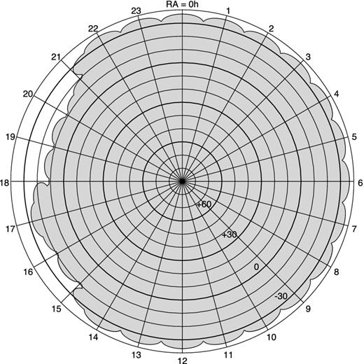
A radial representation of the sky, with areas imaged in the VLSSr shaded. The circles represent declination in 10° increments running from δ = 90° at the centre to δ = −40° at the edge. The radial lines represent hours of RA, increasing clockwise from 0h at the top to 23h.
3.6 Cataloguing
A catalogue of sources was extracted from the mosaic images using the Obit task FndSou to fit Gaussians to peaks in the maps. Sources were searched down to 3.5 times the global rms value in each mosaic image; the catalogue was then filtered to keep only sources at greater than 5σ significance, with the rms noise measured locally in a region with a 60 pixel (15 arcmin) radius.
The final catalogue contains 92 964 entries. Of these, roughly 3 per cent have no match in the NVSS within 60 arcsec of the fitted position. However many unmatched sources are actually components of larger sources which may be fit differently in the two catalogues.
To get a more accurate count of sources with no NVSS counterpart, we filtered out ∼ 90 000 isolated sources. These are sources with no second VLSSr component within 120 arcsec, which is the maximum allowed source size used in the fitting algorithm. Of these isolated sources, 2.2 per cent have no NVSS counterpart within that same 120 arcsec. For the purposes of survey statistics, we consider these false detections.
A 5σ VLSSr source, with peak brightness S74 = 0.5 Jy beam−1 and a spectral index steeper than |$\alpha ^{1400}_{74} = -1.8$|, would fall below the NVSS peak brightness limit of 2.5 mJy beam−1 (Condon et al. 1998). So some fraction of the sources without counterparts may be real, steep-spectrum sources. The rest are generally either noise bumps near 5σ, sidelobes of bright sources, or edge pixels which were corrupted during the mosaic procedure. All of these sources remain in the final catalogue. If there is any doubt about a specific catalogue entry of interest, it can be verified by inspecting the final images.
4 PRIMARY BEAM
During verification of the final catalogue, a flux discrepancy between the previous VLSS and new VLSSr measurements was discovered. We compared unresolved sources to eliminate the effect of the different clean beam sizes and found that the VLSSr sources had, on average, roughly 10 per cent lower measured flux than the sources in the VLSS. Further investigation revealed that the flux deficit was not present in the field maps, before primary beam corrections were made. Re-mosaicking the original VLSS pointing maps using the Obit software also failed to recover the published fluxes. We binned the sources by radial distance from pointing centre, and found there was a clear increase in flux deficit as radius increased (see Fig. 2). This suggested a discrepancy between the primary beam correction used in the previous reduction and the one we were using for the VLSSr.
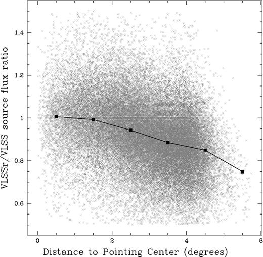
The ratios of the published VLSS flux densities, corrected by a scaled Jinc primary beam, to the VLSSr flux densities corrected with the standard AIPS primary beam function, are plotted as a function of distance to the nearest pointing centre. In order to avoid comparing resolved sources at two different resolutions (80 and 75 arcsec for the VLSS and VLSSr, respectively), only the ∼ 45 000 sources which are unresolved in both catalogues are included. The mean value in 1° radial bins is overlaid on top. The mean ratio for all sources is 0.92.
The standard beam correction for 74 MHz is a polynomial function of Θ, where Θ is defined as the angular offset from the centre of the primary beam. It has a full-width at half-maximum (FWHM) of 11| $_{.}^{\circ}$|8 (Kassim et al. 2007). However, looking at the pipeline code used to reduce the original VLSS, that survey instead used a specialized AIPS-task, WATE, which scaled a Jinc function2 from 1.47 GHz to 74 MHz to get a beam with a FWHM of only 9| $_{.}^{\circ}$|7.
The pointings of the VLSSr overlap sufficiently to provide a source sample for derivation of new primary beam parameters. We used sources observed at multiple pointing radii in the survey data itself to fit a new polynomial for the primary beam. We catalogued all of the pointing images at local 5σ (using σ measured within a 15 arcmin radius of each source), and then searched for isolated sources with no companions within 120 arcsec, which appeared in multiple fields; roughly 92 000 source pairs were identified. To minimize noise the sample was then filtered to include only pairs with both source flux densities >1 Jy and both pointing radii <6° (roughly within the expected FWHM of the beam), and with flux density ratios between 0.3 and 3.5 (to minimize the effect of sources with one severely erroneous measurement). The bright source Cygnus A was also discarded, leaving approximately 10 500 source pairs. We fit a third order polynomial to the ratios of the two flux densities and the two radii for each pair. The fit was weighted by the sum of the flux densities of each pair.
Fig. 3 plots the ratio of source fluxes times the model flux for the source nearest the pointing centre as a function of the distance to the source farthest from the pointing centre. The fitted polynomial is overlaid. Table 2 summarizes the main parameters of the VLSSr beam, the standard AIPS beam, and the VLSS beam.
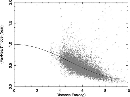
The source pair data used to define a new beam polynomial are plotted as a function of radial distance to the pointing centre of the source which is further from the centre. The polynomial fit is overlaid on the data.
Beam model parameters at 74 MHz.
| Model | Type | Polynomial coefficients | FWHM (deg) |
|---|---|---|---|
| VLSS | Jinc | 9.7 | |
| AIPS | Third ordera | −0.897e-3 | 11.9 |
| 2.71 e-7 | |||
| −0.242e-10 | |||
| VLSSr | Third ordera | −1.051e-3 | 11.2 |
| 4.28e-8 | |||
| −5.38e-11 |
| Model | Type | Polynomial coefficients | FWHM (deg) |
|---|---|---|---|
| VLSS | Jinc | 9.7 | |
| AIPS | Third ordera | −0.897e-3 | 11.9 |
| 2.71 e-7 | |||
| −0.242e-10 | |||
| VLSSr | Third ordera | −1.051e-3 | 11.2 |
| 4.28e-8 | |||
| −5.38e-11 |
aThe third order polynomial has the form: S = 1 + c1xΘ + c2xΘ2 + c3xΘ3, where c1, c2, and c3 are the listed coefficients, and Θ is the distance from the centre of the beam.
In each panel of Fig. 4 we plot the ratio of the source fluxes measured at two different pointing radii as a function of the predicted source flux ratio at those two radii for one of the model beams. The ratios were calculated so that they are always >1.
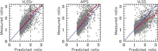
Each panel shows a comparison of the predicted flux ratio at two different pointing radii versus the measured flux ratio at the same radii for a given source. The new VLSSr polynomial fit is on the left, the standard VLA 74 MHz polynomial from AIPS is in the middle and on the right we show the Jinc function used for the VLSS. The blue diagonal line indicates a match between model prediction ratio and measured ratio, while the red triangles indicate the mean measured values. A model ratio of two (indicated with the dashed line) is roughly equivalent to the half power point of the beam.
All three models show reasonable agreement with measured values at a predicted flux ratio of 1; this is expected as the sources in each pair at that ratio must lie at close to identical pointing-centre radii. At larger predicted flux ratios, corresponding to greater radial differences in the positions, the Jinc function used by the VLSS clearly over-predicts the measured flux density ratio. The use of the Jinc function to correct the published VLSS maps thus introduced a radially dependent flux density error.
The standard AIPS polynomial and the newly calculated VLSSr polynomial both show good agreement between the predicted and measured flux density ratios at predicted ratios between 1 and 1.5. Somewhere between predicted ratios of 1.5 and 2, both polynomials start to under-predict the ratio as measured in the data. This problem is more pronounced in the standard AIPS polynomial, particularly at predicted ratios greater than 2. Thus these models will under-predict the flux density of sources at large pointing radii.
A flux density ratio of 2 corresponds, to zeroth order, to a pair of measurements with one at pointing centre and one at the beam radius at full-width half power. Thus both the standard and VLSSr polynomials should be used with caution outside the half-power point of the beam. For this reason we have limited the VLSSr mosaics to data within a radius equivalent to the beam half-power point of each pointing centre.
We are ignoring the known but un-characterized asymmetry of the 74 MHz VLA primary beam (Kassim et al. 2007). Because the pointing images combine snapshots taken over a range of hour angles, we did not feel our images were suitable to investigate the asymmetry. However, it may account for some of the scatter in the plots.
The standard reduction tasks within Obit have been adjusted to include the new VLSSr fitted polynomial beam parameters for 74 MHz, and the fitted beam was used on the final survey products.
5 SURVEY VERIFICATION
5.1 Position errors
The global position offset and errors were measured by comparing measured positions for VLSSr sources to their NVSS positions, following the method previously described in Cohen et al. (2007). We defined a sample of 1284 sources that are weaker than our field calibrators (S < 2.5 Jy) and stronger than 25σ. From these we measure a global position offset of δRA = −0.77 arcsec and δDec = 0.31 arcsec. Catalogue entries have been corrected for this bias.
The global rms position error is 3.3 arcsec in RA and 3.5 arcsec in declination. Positions of individual sources may also be in error due to the Gaussian fitting technique we use, as described in Cohen et al. (2007) and Condon (1997). For each catalogue source, the calculated Gaussian errors are added in quadrature with the global rms position errors to derive the reported catalogue position errors. However, true position errors for any individual source in the VLSSr catalogues will be dominated by residual errors from the ionospheric corrections. These errors are not suited to a global correction as they will vary greatly from location to location, but may be on the order of tens of arcseconds.
5.2 Flux density errors
In order to estimate the uncertainty in measured flux densities for sources in the VLSS, we imaged all of the individual 20 min snapshots for each pointing, and catalogued the sources in them at a >5σ significance. This gave us multiple peak flux density measurements for each source. We then compared the source peak flux density to its mean for each source. We find an average peak flux error of 12 per cent for point sources, and 15 per cent for extended sources. We have included the point source error in the reported catalogue source error values.
The reported errors in the catalogue also include the errors introduced by the Gaussian fits, described in detail in Cohen et al. (2007).
5.3 Flux scale
During the course of investigating the primary beam-model, we also tested our processing steps to see if they introduced any flux scale bias. We found that, with the exception of fields with extreme RFI, the RFI filtering and flagging steps were reducing source fluxes in the maps by ∼ 5 per cent. Tests run independently on the filtering versus the flagging step showed that both steps contribute to the flux loss.
The original VLSS is assumed to lie on a Baars et al. scale (Baars et al. 1977), because the primary calibration is tied to the Baars et al. model for Cygnus A. While some comparisons were made to existing source fluxes [notably to Kühr et al. models (Kühr et al. 1981) and the 8C/6C catalogues (Rees 1990; Hales et al. 1991)], the conclusion made was that no flux bias existed within the flux errors of the catalogues used (Cohen et al. 2007). However the Kühr et al. models are not always reliable at low frequencies (particularly for weaker sources) when there are few existing low frequency measurements in the literature, and the 8C/6C catalogues are not themselves on the Baars et al. scale.
When we investigated the existing low frequency catalogues to generate expected fluxes at 74 MHz to measure the flux bias in the VLSSr, we found that the majority had been placed on the Roger et al. (1973, RCB) scale. This scale has the advantage over the Baars et al. scale that it is based on low frequency flux measurements and thus consistent down to the lowest frequencies. The Baars et al. scale is tied to models of Cas A and Cygnus A which are not accurate at very low frequencies.
We compared the model predictions of all six bright 3C sources found in Scaife & Heald (2012) to the integrated flux densities in the VLSSr to calculate an average flux density correction for our survey, and place it on to the RCB scale. A summary of the predicted and measured integrated flux densities for the six sources is given in Table 3. The average correction factor was 1.10x. This scaling was applied to the VLSSr image mosaics before cataloguing. When using the VLSSr in conjunction with higher frequency, Baars et al. scale catalogues, the scaling can be reversed; however, we suggest that the assumed uncertainty in the flux measurement (discussed in Section 5.2) should be increased by ∼ 5 per cent to reflect the known biases of the reduction method as discussed above.
Scaife & Heald source model parameters.
| Source | Model order | Predicted | Raw VLSSr | Ratio |
|---|---|---|---|---|
| Jy beam−1 | Jy beam−1 | |||
| 3C48 | 3rd | 77 | 69 | 1.12 |
| 3C147 | 3rd | 52 | 52 | 1.0 |
| 3C196 | 2nd | 133 | 121 | 1.10 |
| 3C286 | 3rd | 31 | 28 | 1.11 |
| 3C295 | 4th | 132 | 121 | 1.09 |
| 3C380 | 1st | 133 | 112 | 1.19 |
In Fig. 5, we compare VLSSr flux densities to those predicted by interpolating between the 6C (151 MHz; Hales et al. 1991) and 8C (38 MHz; Rees 1990) catalogues.
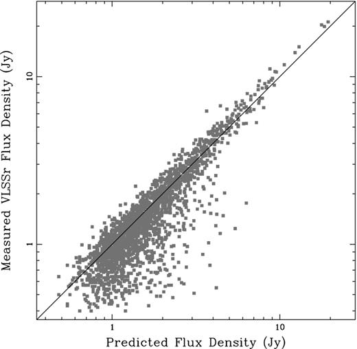
A comparison of predicted and measure flux density for 2096 isolated, unresolved VLSSr sources with matches in the 6C and 8C catalogues. The predicted flux densities were calculated at 73.8 MHz by interpolating between the 6C (151 MHz) and 8C (38 MHz) flux densities. The line indicates a ratio between predicted and measured flux densities of unity.
The 8C beam is 4.5 × 4.5csc(δ) arcmin; at a declination of δ = 60° this corresponds to 4.5 × 5.2 arcmin. The 6C beam is only slightly smaller, at 4 × 4csc(δ) arcmin. However, the VLSSr beam is only 1.25 arcmin. In order to compare flux density between the three catalogues, we constructed a sample of isolated, unresolved sources. We require that all sources be present in all three catalogues.
For the 8C catalogue we required that sources have the descriptor ‘P’ for point source. We used the integrated flux density when available, and peak intensity when it was not (peak intensity for an unresolved point source should be the same as integrated flux density). For the 6C sources, we required that they not be marked as part of a source complex. As with the 8C catalogue, we used integrated flux density when available and peak flux density for the remaining sources.
For the VLSSr we used the deconvolved total source flux density, which includes the clean bias correction. We required that the VLSSr have only one source entry within a 6 arcmin radius of the reported 8C source position to ensure that we were comparing single isolated sources. Finally we required that the source be unresolved in the VLSSr, with only upper limits for the deconvolved source major and minor axes.
For the sample of 2096 sources thus selected the median ratio of measured VLSSr to predicted flux density is 0.92. There is a trend for the VLSSr to be below the prediction at lower flux densities and above the prediction at higher flux densities. Thus for the 231 sources with S74 ≥ 3 Jy, the median ratio of measured to predicted flux densities is 1.07, while for the 674 sources with S74 < 1 Jy, the median ratio of measured to predicted flux density is only 0.72. It is uncertain what might cause this flux-dependent scale variation; however it is clear that the weakest sources, in particular, are not reliable in this comparison. If we limit the sample to sources with S74 > 1 Jy, the median ratio of measured to predicted flux density is 0.97.
6 SKY AREA IMAGED
In Fig. 1, we show the sky coverage of the VLSSr. The survey covers roughly 3π sr, equivalent to the intended area of the original observations. The resulting images completely cover declinations δ > −10° for 18h < RA < 21h and δ > −20° for 15h < RA < 18h. The lower declination fields at these right ascensions were corrupted and the data could not be imaged. The remainder of the sky is covered for all declinations δ > −30°, with a scalloped edge extending to δ ≃ −36°.
7 SKY NOISE PROPERTIES
The average rms noise over the entire survey area is σ = 0.1 Jy beam−1. Fig. 6 indicates how much sky was observed at a given rms noise level. The majority of the survey has an rms within ±0.03 Jy beam−1 around the median noise level of 0.095 Jy beam−1, with a long tail of larger rms values. This tail comprises largely regions near very strong sources where sidelobes raise the local noise level. It also includes regions near the edge of the survey area where there is no neighbouring field to improve the sensitivity, and regions located along the higher temperature Galactic plane. Finally it includes some areas where the ionospheric calibration was poor due either to a lack of calibrator sources or unusually bad ionospheric weather.
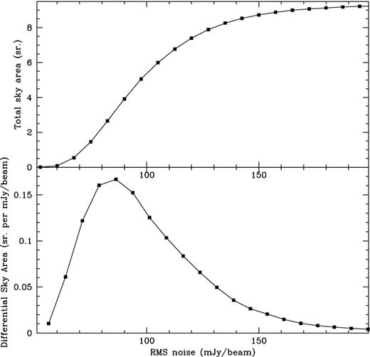
Top: total sky area in steradians (y-axis) at or below a given rms noise level (x-axis). The mean noise level is 0.1 Jy beam−1. Values have been measured from residual (source-subtracted) images. Bottom: the differential sky area in steradians per Jy beam−1.
8 SOURCE SPECTRAL INDICES
We calculated an average spectral index to 1400 MHz, using the NVSS (Condon et al. 1998) for flux values. We started with ∼ 90 000 isolated VLSSr sources with no additional source in a 120 arcsec radius, and searched for NVSS matches within the same 120 arcsec radius. After removing sources with more than one NVSS match, we were left with 67 844 unique source pairs. We divided the VLSSr flux densities by 1.1 to re-place them on to the default Baars et al. scale used by the NVSS, and calculated spectral index values for each source. The median spectral index is |$\alpha ^{1400}_{74} = -0.82$|. The spread in the derived median, represented by the semi-inter-quartile range, is SIQR = 0.11.
Fig. 7 shows the spectral index distribution, which is reasonably symmetric. The median agrees within the errors with the median spectral index of |$\alpha ^{1400}_{325} \sim -0.9$| found between bright WENSS sources and the NVSS by Zhang et al. (2003), and the value of |$\alpha ^{1400}_{74} \sim -0.72$| found for the bright sample in a deep low frequency study of the XMM-LSS field (Tasse et al. 2006).
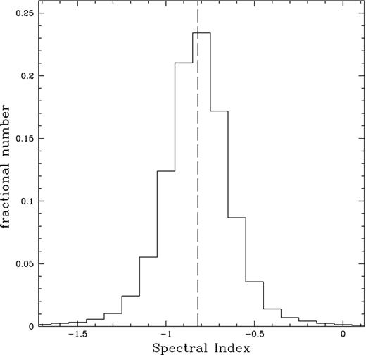
Histogram showing the spectral index distribution for sources from the VLSSr compared to the NVSS (1400 MHz, black). The median spectral index, |$\alpha ^{1400}_{74} = -0.82,$| is shown with a dashed line.
9 log N − log S
We used the cumulative distribution of rms noise seen in Fig. 6 to derive the differential source counts for the 92 964 sources in our catalogue. For each source, we compute Amax, the total area for which Fp > 5σ (where Fp is the peak flux and σ is the local rms noise as computed in the cataloguing step; see Section 3.6).
When the mean weight, N−1∑Amax, is unity, we compute the uncertainty using Poisson statistics (Gehrels 1986). The results are tabulated in Table 4.
Source count data for the VLSSr. Tabulated values are on the RCB flux scale.
| Flux range | log10Sc | Raw counts | Mean area | Mean weight | Normalized counts |
|---|---|---|---|---|---|
| (Jy) | (Jy) | (sr) | (103 Jy3/2 sr−1) | ||
| 0.39–0.53 | −0.32 | 5813 | 2.4 | 0.17 | |$\phantom{1}3.7^{+0.1}_{-0.1}$| |
| 0.53–0.72 | −0.20 | 16490 | 5.6 | 0.53 | |$\phantom{1}5.4^{+0.0}_{-0.0}$| |
| 0.72–0.98 | −0.08 | 18825 | 8.1 | 0.85 | |$\phantom{1}6.1^{+0.0}_{-0.0}$| |
| 0.98–1.33 | 0.05 | 16129 | 9.0 | 0.97 | |$\phantom{1}7.3^{+0.1}_{-0.1}$| |
| 1.33–1.81 | 0.19 | 11423 | 9.3 | 0.99 | |$\phantom{1}8.0^{+0.1}_{-0.1}$| |
| 1.81–2.47 | 0.32 | 8332 | 9.3 | 1.00 | |$\phantom{1}9.2^{+0.1}_{-0.1}$| |
| 2.47–3.36 | 0.45 | 5768 | 9.3 | 1.00 | |$10.1^{+0.1}_{-0.1}$| |
| 3.36–4.57 | 0.58 | 3755 | 9.3 | 1.00 | |$10.4^{+0.2}_{-0.2}$| |
| 4.57–6.22 | 0.72 | 2411 | 9.3 | 1.00 | |$10.6^{+0.2}_{-0.2}$| |
| 6.22–8.46 | 0.85 | 1457 | 9.3 | 1.00 | |$10.2^{+0.3}_{-0.3}$| |
| 8.46–11.5 | 0.98 | 864 | 9.3 | 1.00 | |$\phantom{1}9.6^{+0.3}_{-0.3}$| |
| 11.5–15.7 | 1.12 | 504 | 9.3 | 1.00 | |$\phantom{1}8.9^{+0.4}_{-0.4}$| |
| 15.7–21.3 | 1.26 | 260 | 9.3 | 1.00 | |$\phantom{1}7.2^{+0.5}_{-0.4}$| |
| 21.3–29.0 | 1.39 | 138 | 9.3 | 1.00 | |$\phantom{1}6.1^{+0.6}_{-0.5}$| |
| 29.0–39.5 | 1.52 | 95 | 9.3 | 1.00 | |$\phantom{1}6.7^{+0.8}_{-0.7}$| |
| 39.5–53.7 | 1.66 | 45 | 9.3 | 1.00 | |$\phantom{1}5.0^{+0.9}_{-0.7}$| |
| 53.7–73.0 | 1.77 | 24 | 9.3 | 1.00 | |$\phantom{1}4.2^{+1.1}_{-0.9}$| |
| 73.0–99.4 | 1.95 | 7 | 9.3 | 1.00 | |$\phantom{1}2.0^{+1.1}_{-0.7}$| |
| 99.4–135 | 2.09 | 12 | 9.3 | 1.00 | |$\phantom{1}5.3^{+2.1}_{-1.5}$| |
| 135–184 | 2.20 | 6 | 9.3 | 1.00 | |$\phantom{1}4.2^{+2.6}_{-1.7}$| |
| 184–250 | 2.28 | 2 | 9.3 | 1.00 | |$\phantom{1}2.2^{+3.1}_{-1.4}$| |
| 250–341 | 2.52 | 1 | 9.3 | 1.00 | |$\phantom{1}1.8^{+4.3}_{-1.5}$| |
| 341–464 | 2.63 | 3 | 9.3 | 1.00 | |$\phantom{1}8.5^{+8.5}_{-4.6}$| |
| 464–631 | 2.71 | 2 | 9.3 | 1.00 | |$\phantom{1}9.0^{+12.3}_{-5.8}$| |
| 631–858 | 2.80 | 1 | 9.3 | 1.00 | |$\phantom{1}7.1^{+17.2}_{-5.9}$| |
| 858–1168 | 2.97 | 1 | 9.3 | 1.00 | |$11.3^{+27.3}_{-9.4}$| |
Source count data for the VLSSr. Tabulated values are on the Baars et al. flux scale. Data above the line have been used in Fig. 8, while those below the line were excluded from the figure due to small source number counts.
| Flux range | log10Sc | Raw counts | Mean area | Mean weight | Normalized counts |
|---|---|---|---|---|---|
| (Jy) | (Jy) | (sr) | (103 Jy3/2 sr−1) | ||
| 0.39–0.53 | −0.33 | 9402 | 3.4 | 0.27 | |$\phantom{1}3.8^{+0.1}_{-0.1}$| |
| 0.53–0.72 | −0.20 | 18049 | 6.6 | 0.65 | |$\phantom{1}4.8^{+0.0}_{-0.0}$| |
| 0.72–0.98 | −0.08 | 18508 | 8.5 | 0.90 | |$\phantom{1}5.6^{+0.0}_{-0.0}$| |
| 0.98–1.33 | 0.05 | 14324 | 9.1 | 0.98 | |$\phantom{1}6.4^{+0.1}_{-0.1}$| |
| 1.33–1.81 | 0.19 | 10420 | 9.3 | 1.00 | |$\phantom{1}7.2^{+0.1}_{-0.1}$| |
| 1.81–2.47 | 0.32 | 7535 | 9.3 | 1.00 | |$\phantom{1}8.3^{+0.1}_{-0.1}$| |
| 2.47–3.36 | 0.45 | 5139 | 9.3 | 1.00 | |$\phantom{1}9.0^{+0.1}_{-0.1}$| |
| 3.36–4.57 | 0.58 | 3244 | 9.3 | 1.00 | |$\phantom{1}9.0^{+0.2}_{-0.2}$| |
| 4.57–6.22 | 0.72 | 2102 | 9.3 | 1.00 | |$\phantom{1}9.2^{+0.2}_{-0.2}$| |
| 6.22–8.46 | 0.85 | 1232 | 9.3 | 1.00 | |$\phantom{1}8.6^{+0.3}_{-0.2}$| |
| 8.46–11.5 | 0.98 | 706 | 9.3 | 1.00 | |$\phantom{1}7.8^{+0.3}_{-0.3}$| |
| 11.5–15.7 | 1.12 | 430 | 9.3 | 1.00 | |$\phantom{1}7.6^{+0.4}_{-0.4}$| |
| 15.7–21.3 | 1.25 | 212 | 9.3 | 1.00 | |$\phantom{1}5.9^{+0.4}_{-0.4}$| |
| 21.3–29.0 | 1.39 | 120 | 9.3 | 1.00 | |$\phantom{1}5.3^{+0.5}_{-0.5}$| |
| 29.0–39.5 | 1.51 | 77 | 9.3 | 1.00 | |$\phantom{1}5.4^{+0.7}_{-0.6}$| |
| 39.5–53.7 | 1.65 | 41 | 9.3 | 1.00 | |$\phantom{1}4.6^{+0.8}_{-0.7}$| |
| 53.7–73.0 | 1.80 | 13 | 9.3 | 1.00 | |$\phantom{1}2.3^{+0.8}_{-0.6}$| |
| 73.0–99.4 | 1.93 | 8 | 9.3 | 1.00 | |$\phantom{1}2.2^{+1.1}_{-0.8}$| |
| 99.4–135 | 2.06 | 11 | 9.3 | 1.00 | |$\phantom{1}4.9^{+2.0}_{-1.5}$| |
| 135–184 | 2.21 | 6 | 9.3 | 1.00 | |$\phantom{1}4.2^{+2.6}_{-1.7}$| |
| 250–341 | 2.48 | 1 | 9.3 | 1.00 | |$\phantom{1}1.8^{+4.3}_{-1.5}$| |
| 341–464 | 2.60 | 4 | 9.3 | 1.00 | |$11.3^{+9.2}_{-5.4}$| |
| 464–631 | 2.73 | 2 | 9.3 | 1.00 | |$\phantom{1}9.0^{+12.3}_{-5.8}$| |
| 631–858 | 2.93 | 1 | 9.3 | 1.00 | |$\phantom{1}7.1^{+17.2}_{-5.9}$| |
In order to compare our source counts to those found in other sky surveys, we have scaled the VLSSr to the Baars et al. flux scale and recalculated the counts (see Table 5). In Fig. 8 we plot the results. We have excluded VLSSr flux bins with fewer than 20 sources from the figure.
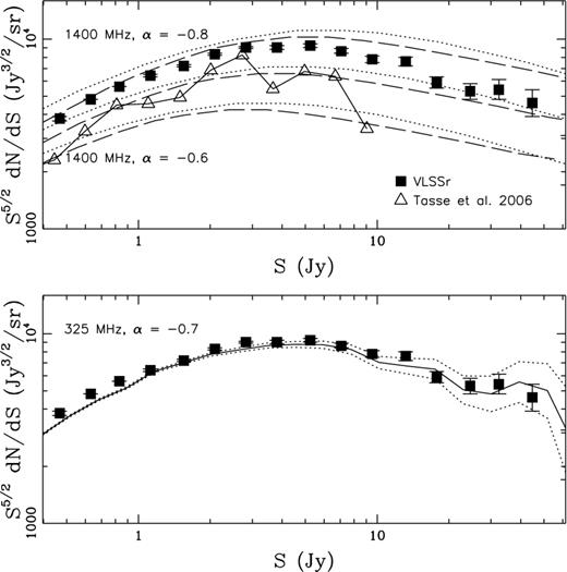
Euclidean-normalized source counts for the VLSSr are shown, scaled on to the Baars et al. flux scale. Top: VLSSr counts (squares) are overlaid on curves from the 1.4 GHz source counts given in Condon (dotted line, 1984) and Seymour et al. (dashed line, 2004). The 1.4 GHz curves have been scaled to 74 MHz by spectral indices of α = −0.6, −0.7 and −0.8. We also plot values for 74 MHz counts taken from Tasse et al. (triangles, 2006). Bottom: VLSSr counts are overlaid on a curve derived from WENSS sources (Rengelink et al. 1997) and scaled to 74 MHz by a spectral index of α = −0.7 ± 0.3. Errors in the WENSS counts are indicated by the dotted lines.
In the top panel we have plotted our source counts and overlaid curves taken from the 1.4 GHz source counts in Condon (1984) and Seymour, McHardy & Gunn (2004), which have been extrapolated to 74 MHz using a range of assumed spectral indices. At low and moderate flux values our counts are in reasonable agreement with the extrapolated curve using |$\alpha ^{1400}_{74} = -0.8$|; this in turn agrees well with the median spectral index found previously between the VLSSr and NVSS. At higher flux values we find a steeper drop-off than seen in the 1.4 GHz curve.
Tasse et al. (2006) previously used a deep study of the XMM-LSS field to calculate source counts at 74 MHz. Their counts, based on ∼ 650 sources observed at higher resolution than the VLSSr (Θ ∼ 30 arcsec), are overlaid on the top panel. We have left off the error bars to simplify the display. The Tasse curve falls below the VLSSr curve, but, when compared to the 1400 MHz counts, it is consistent with the lower mean spectral index (|$\alpha ^{1400}_{74} = -0.72$|) they also derive.
In the bottom panel the overlaid curve is derived from an analysis of the 325 MHz WENSS catalogue (Rengelink et al. 1997), with the 1σ Poisson uncertainty indicated by the dotted curves. We used the calculated spectral index and scatter between VLSSr (on the Baars et al. scale) and WENSS (α = −0.7 ± 0.3) to assign a 74 MHz flux to each WENSS source. The source count that is obtained using this Monte Carlo method is in good agreement with the VLSSr curve.
10 VLSS VERSUS VLSSr
The VLSS catalogue and images were limited by the available software and computer processing power, as well as a lack of a same-frequency initial sky model for the ionospheric calibration step. The VLSSr reduction took advantage of experience gained from the VLSS itself to improve the final data products in many areas. Fig. 9 shows a sample extended source imaged by both surveys, and Table 6 summarizes the main survey parameters for each.
Comparison of VLSS and VLSSr processing.
| Property | VLSS | VLSSr |
|---|---|---|
| Clean beam (FWHM) | 80 arcsec | 75 arcsec |
| Pixel scale | 25 arcsec | 15 arcsec |
| Mean rms (Jy beam−1)a | 0.12 | 0.09 |
| Clean bias | 1.39σ | 0.66σ |
| Largest angular size | 18 arcmin | 36 arcmin |
| Total sky area (sr) | 9.43 | 9.38 |
| Sources detected (≥5σ) | 68 311 | 92 964 |
| Catalogue non-match rate | 1 per cent | 2.2 per cent |
arms is quoted using the Baars et al. scale for both. On the Scaife & Heald (2012) scale, the mean rms of the VLSSr is σ ∼ 0.1 Jy beam−1.
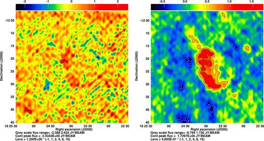
A comparison of the supernova remnant Kes 63 in the VLSS (left) and VLSSr (right) processing.
The VLSSr uses a slightly smaller clean beam (75 arcsec) and pixel scale (15 arcsec) compared to the VLSS. We felt the smaller beam was a more accurate reflection of the natural data properties, and the pixel scale was lowered to provide 5 pixels resolution across the beam.
The VLSSr processing took advantage of a new smart-windowing algorithm to clean only areas in the images that have real sources and avoid cleaning noise bumps (Cotton 2007; Lane et al. 2012). When noise is cleaned, flux is subtracted from real sources, introducing a flux bias which scales with the local rms noise. The point source clean-bias in the VLSSr is 0.66σ, where σ is the locally measured rms noise in the image. This is slightly less than half the clean-bias from the VLSS. The online catalogue corrects for the clean-bias in the deconvolved flux values.
Improved RFI-removal algorithms for the VLSSr allow the inclusion of all short baselines present in the data. In order to mitigate RFI which tends to affect short baselines more than longer baselines, the VLSS processing removed all baselines shorter than 200λ. By keeping the short baselines, the VLSSr doubles the theoretical largest angular size (LAS) imaged to 36 arcmin. Short observations with poor uv-coverage will reduce the actual angular size measured in the maps. The observations were spread out in hour angle as much as possible to mitigate this effect; however it is probable that the maximum LAS was not reached in all areas on the sky.
Because of the ionospheric phase calibration improvements from using a same-frequency sky catalogue, we were able to process all fields for the VLSSr without doing any initial self-calibration. In the VLSS this step was necessary for many fields to be imaged at all. While a small number of VLSSr fields have visible calibration issues (distorted source shapes or doubled sources are the most common) which may have been ameliorated by the self-calibration step, we preferred to avoid the hybrid phase treatment of self-calibration followed by field-calibration.
The improvements in ionospheric calibration and RFI removal lead to substantially better final images. If we scale the VLSSr to the Baars et al. flux scale to make a comparison, the average rms noise has decreased by a factor of 25 per cent in the VLSSr to σ = 0.09 Jy beam−1. Higher-declination holes in the VLSS coverage area have been filled in by the VLSSr, and sensitivity to large sources (e.g. Galactic supernova remnants) is greatly improved.
In the original VLSS survey, a comparison of 200 sources with S74 > 4 Jy had an average ratio of measured VLSS flux to flux predicted by extrapolating between the 6C and 8C catalogues of ∼ 0.99 with a 10 per cent rms scatter (Cohen et al. 2007). By comparison, the same ratio is ∼ 1.07 with a 13 per cent rms scatter for the roughly 230 unresolved sources in the VLSSr S74 ≥ 3 Jy. While it is clear that the VLSS appears to be in better agreement with the prediction for these bright sources, we note that no effort was made to ensure that the VLSS sample was restricted to unresolved sources, so the comparison included extended sources measured with very different beams. The VLSS result was also affected by the known position-dependent flux errors in that catalogue.
The VLSSr rate of unmatched sources is higher than for the original VLSS, with 2.2 per cent of isolated VLSSr sources having no NVSS counterpart within 120 arcsec, compared to ≤1 per cent in the VLSS. One reason is that the VLSS filtered the catalogue to require a higher significance for inclusion near bright sources in an effort to reduce the inclusion of sidelobes from sources (Cohen et al. 2007). Because nearly half of the sources removed by this filter were real (had NVSS counterparts), we chose not to use this filter for the VLSSr.
A final major improvement is the use of a more accurate primary beam correction for the VLSSr. A comparison of the VLSS and VLSSr primary beams is shown in Fig. 10. The primary beam correction for the VLSS over-corrected source fluxes, with the size of the error changed with radial distance to closest pointing centre. As a result, while the global flux scale for the VLSS looked quite reasonable when compared to literature spectra and source flux values, measurements of a given source could be wrong by a factor which varied by source location. Correction of the primary beam shape for the VLSSr provides substantially more reliable and uniform source flux measurements and removes the radially dependent flux errors.
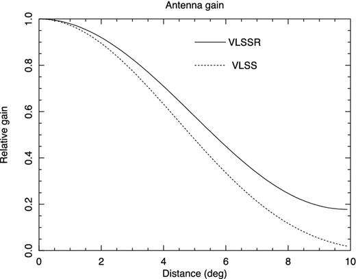
The scaled Jinc shaped-beam used to correct the VLSS versus the fitted polynomial beam used for the VLSSr as a function of radius. The two beams show a clear discrepancy which increases with increasing radius.
11 CONCLUSIONS
The VLSSr provides a more accurate and more detailed map of the sky at 74 MHz than the original VLSS. The improved sensitivity is reflected in greater detail on images of faint structures. The increased angular scale allows measurements of supernova remnants and other large sources not visible in the final VLSS images.
We have derived an improved primary beam model for the 74 MHz VLA, based on sources observed multiple times in adjacent pointings. The new model is implemented in the Obit software reduction package. We have used it to correct a substantial primary beam error in the original VLSS.
In keeping with other low-frequency catalogues we have placed the survey on to the RCB scale (Roger et al. 1973), using the source models from Scaife & Heald (2012). Those who wish to compare VLSSr data to higher frequencies can re-place the survey products on to the Baars et al. (1977) scale, by dividing all fluxes by a factor of 1.1.
All data (images and catalogue) are publicly available at: http://www.cv.nrao.edu/vlss/VLSSpostage.shtml.
Basic research at the Naval Research Lab is supported by 6.1 base funds. We thank E. Polisensky for help with the graphics. Part of this research was carried out at the Jet Propulsion Laboratory, California Institute of Technology, under a contract with the National Aeronautics and Space Administration. The National Radio Astronomy Observatory is a facility of the National Science Foundation operated under cooperative agreement by Associated Universities, Inc.
Where Sν ∝ να.
Defined as |$J_{\rm inc}(t) = {J_{1}(t)\over {t}}$|, where J1(t) is a Bessel function of the first kind.
REFERENCES
SUPPORTING INFORMATION
Additional Supporting Information may be found in the online version of this article:
Table 1. Notes on Individual Pointings.
Please note: Oxford University Press are not responsible for the content or functionality of any supporting materials supplied by the authors. Any queries (other than missing material) should be directed to the corresponding author for the article.
