A Common “Stripmap-Like” Interferometric Processing Chain for TOPS and ScanSAR Wide Swath Mode


1
Lyles School of Civil Engineering, Purdue University, West Lafayette, IN 47906, USA
2
School of Mechanical Engineering, Northwestern Polytechnical University, Xi’an 710072, China
*
Author to whom correspondence should be addressed.
Remote Sens. 2018, 10(10), 1504; https://doi.org/10.3390/rs10101504
Submission received: 3 August 2018
/
Revised: 7 September 2018
/
Accepted: 10 September 2018
/
Published: 20 September 2018
(This article belongs to the Section Remote Sensing Image Processing)
Abstract
:This article describes the technical implementation of a “stripmap-like” interferometric processing flow that could be used for both Terrain Observation with Progressive Scans (TOPS) and ScanSAR. In this “stripmap-like” approach, the discontinuous bursts of wide swath mode for the same subswath are stitched into a continuous single look complex (SLC) image at the very beginning of the processing chain. For users who wish not to get into the complexity behind the wide swath mode and simply want to use the interferometric products, this implementation provides the identical processing steps and output products to the stripmap case. This implementation also features a user-friendly processing interface, where all the wide-swath-related processes are hidden under the hood. In addition, this approach makes the best use of an existing standard InSAR processing software. In this article, the complete common processing chain for TOPS and ScanSAR is elaborated and some key issues are discussed, starting from stitching, deramping to coregistration and enhanced spectral diversity (ESD). The authors also introduce a quick implementation of fine coregistration during the ESD step that does not require resampling the slave image using the conventional method.
1. Introduction
1.1. An Introduction to ScanSAR and TOPS
In the conventional stripmap mode, the range width is restrained by the pulse repetition frequency (PRF), nadir return and received window timing [1]. For the purpose of scanning larger areas by increasing swath width, in 1981, Tomiyasu [2] and Moore [3] proposed the ScanSAR mode. The name ScanSAR comes from the “scanning” antenna in different swaths as a trade-off to azimuth resolution. Nowadays, ScanSAR is widely implemented in most of the synthetic aperture radar (SAR) sensors including RADARSAT, Envisat, TerraSAR-X, COSMO, ALOS and ALOS-2.
The ScanSAR system is not initially designed for interferometry. It was not until the 1990s when Politecnico di Milano [4] and German Aerospace Center [5] started relevant work. One of the most successful ScanSAR interferometric applications is the SRTM mission in 2000 [6], where the global topography was mapped in an 11-day mission. In 2005, the European Space Agency (ESA) started to release ScanSAR single look complex (SLC) products for the interferometric purpose.
However, despite the long history of ScanSAR interferometry, its scientific studies and applications are very limited for a few reasons. To start with, the first generation ScanSAR, such as Envisat ASAR, has a very low spatial resolution (8 m slant range × 80 m azimuth). The low resolution makes the speckle effect worse and hence restricts the application scope for interferometry. Secondly, Envisat ScanSAR has limited ability to control burst synchronization [7,8]. This will lead to a loss in the azimuth common bandwidth and decorrelation in the interferogram [9]. Another issue with the ScanSAR system for the interferometric purpose is the scalloping effect [10]. In ScanSAR mode, ground targets in different azimuth positions are illuminated by the different portions of the azimuth antenna beam pattern (AAP). As a result, the received signal-to-noise ratio (SNR) become azimuth dependent. While the amplitude modulation in the scalloping effect could be compensated by multilook, it would be very unlikely to correct the azimuth-dependent SNR for interferometric purpose [4,10]. A low SNR at the edges of the bursts will decrease the coherence in interferometry. The Terrain Observation with Progressive Scans (TOPS) mode is proposed to minimize this scalloping effect in interferometry.
In the TOPS mode, the antenna sweeps in the opposite direction to a spotlight (SPOT) mode, hence the name “TOPS” [10]. In the ScanSAR mode, the antenna only switches between different subswaths but does not “sweep” in azimuth. In the TOPS mode, the antenna “sweeps” in the azimuth direction back and forth in each subswath so that all targets are scanned by the entire AAP, hence their amplitude gains are at the same level. There is still a minor scalloping effect in TOPS, but it is mainly due to phase array steering and grating lobes [11,12]. The ESA distributed SLC data has also corrected this effect [13].
This new acquisition mode was firstly tested on the German satellite TerraSAR-X for validation [14,15,16]. Then, in 2014, the Sentinel-1 (S1) mission made TOPS famous by setting TOPS as the default acquisition mode and by making the data free to the public. Compared with Envisat ScanSAR, S1 increases the azimuth resolution to 20 m, decreases revisit time to 12 days, tightens the orbital to a 200 m tube to favor interferometry [13]. At last, S1 achieves a perfect timing control, baseline control and burst synchronization so that the temporal, geometrical and spectral decorrelation could be minimized [13,17]. The superb control of S1 burst synchronization means that, in most cases, there will be no significant coherence loss even if no filtering in azimuth is performed [18]. Unlike its ancestors, every detail in S1 TOPS mode is aimed at doing interferometry [19,20].
1.2. A “Stripmap-like” Processing Chain for TOPS and ScanSAR
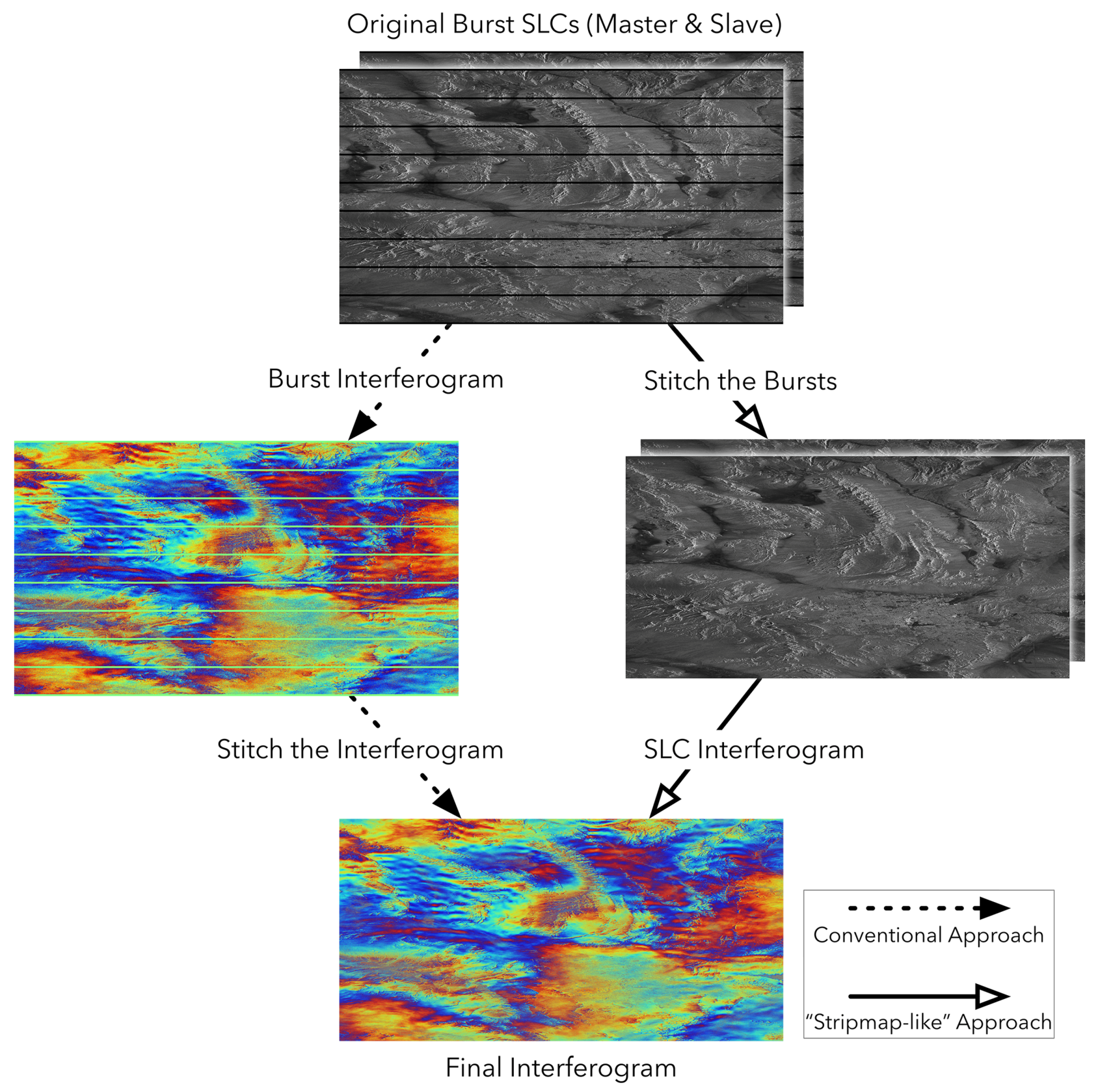
Despite the increasing popularity of the wide swath mode, the interferometric process is still more complicated than the stripmap mode. For users who only have the basic familiarity with the stripmap mode, and simply wish to derive the interferometric product for their own Earth Observation (EO) applications, the burst mode of wide swath looks quite counterintuitive. This is because the burst mode SLC is not continuous in the azimuth (see Figure 1, Figure 2 and Figure 3), making it very different from the stripmap case and harder to interpret. In addition, the wide swath mode requires extra steps in the coregistration, including deramping/reramping and enhanced spectral diversity (ESD), that requires some fundamental understanding to the signal characteristics of the wide swath mode.
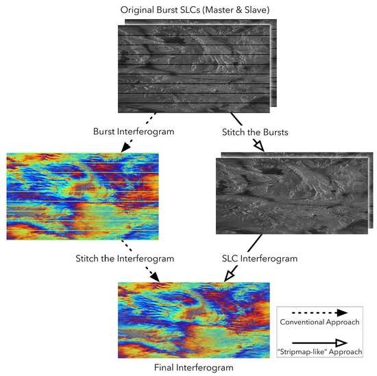
Currently, one approach that is widely adopted in the SAR community for processing the wide swath mode (including both ScanSAR and TOPS) is to process each burst individually and to generate the burst interferogram. The burst interferogram is stitched into the continuous interferogram at the very last step. Examples of this approach are [21,22] for ScanSAR, and [18,23] for TOPS. The advantage of this approach is that it is straightforward to think about and easy to implement. One starts by reading in the burst mode SLC image. The coregistration (using the geometrical approach [24]) and the ESD steps are all performed on the individual bursts. It should be noted that, although there are overlapping areas between adjacent bursts, they are not redundant information because they have different phase values. For this approach, the bursts are kept intact and no signals (for the overlaps between bursts) are thrown away. As the signals from the overlaps are required in the ESD step, they could be read conveniently from the resampled burst SLC. The burst interferogram is then generated from the resampled burst SLCs. The software development complexity for this approach is lower. An illustration of this approach is shown in Figure 1.
In this article, we propose another approach, which is to generate a continuous SLC image, identical to a stripmap SLC image, at the very beginning of the processing chain. The initiative of this approach is to provide a more user-friendly interface for users who do not wish to understand all the theories and processing steps of the wide swath mode, i.e., burst mode, stitching (in some literature this is referred as “debursting” [23]), deramping, ESD, etc. Users will start by seeing the images (amplitude) exactly the same as for the stripmap mode. All the processing steps and outcomes (SLCs and interferograms) are identical to the stripmap case. For non-expert users, no extra steps or knowledge are required for data processing, and no difference will be noticed in the processing software interface. The wide-swath-related processes are implemented under the hood. Anyone with the basic understanding of stripmap interferometric processing flow could also process wide swath mode with this interface and processing flow, and derive interferometric/time series analysis products. In addition, the stripmap-like processing chain would take advantage of an existing and mature stripmap processing platform. The integration between the proposed processing flow for wide swath and existing stripmap processor would be more convenient in the aspects of processing platform development and maintenance. An illustration of this approach is shown in Figure 1.
Stitching bursts into a continuous SLC at the very first step is not entirely a new idea. In the past, some software also implemented similar ideas [25,26]. However, very few technical details were revealed in those references. In [27]’s paper, the author also implemented a very similar idea, but a lot of the details deviate from what will be discussed in this article. For example, in [27]’s paper, the author only performed the deramping process and modulated the signal to the baseband, but, in this study, we will still reramp the signal after the initial coregistration. The reason will be discussed in the next section.
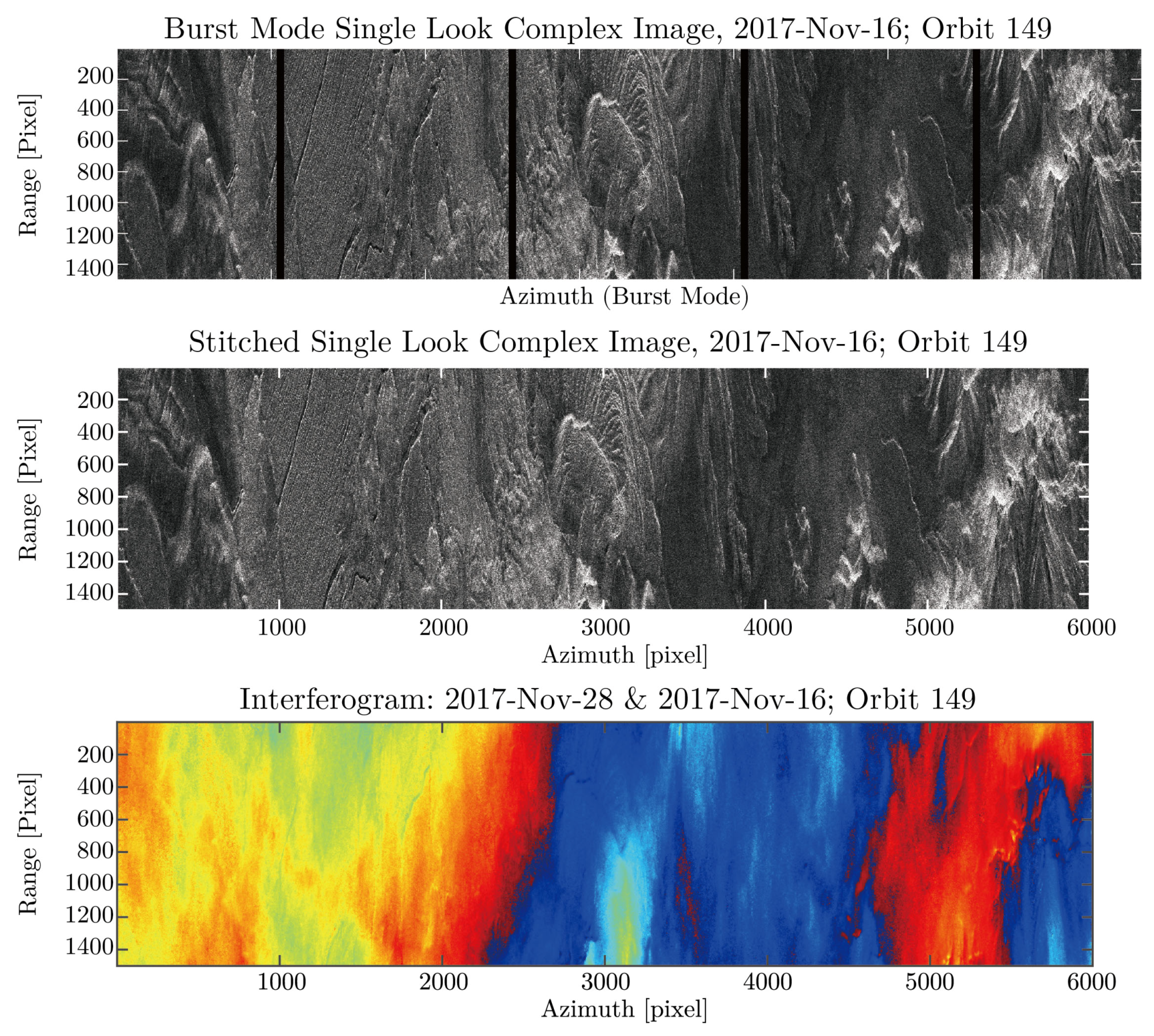
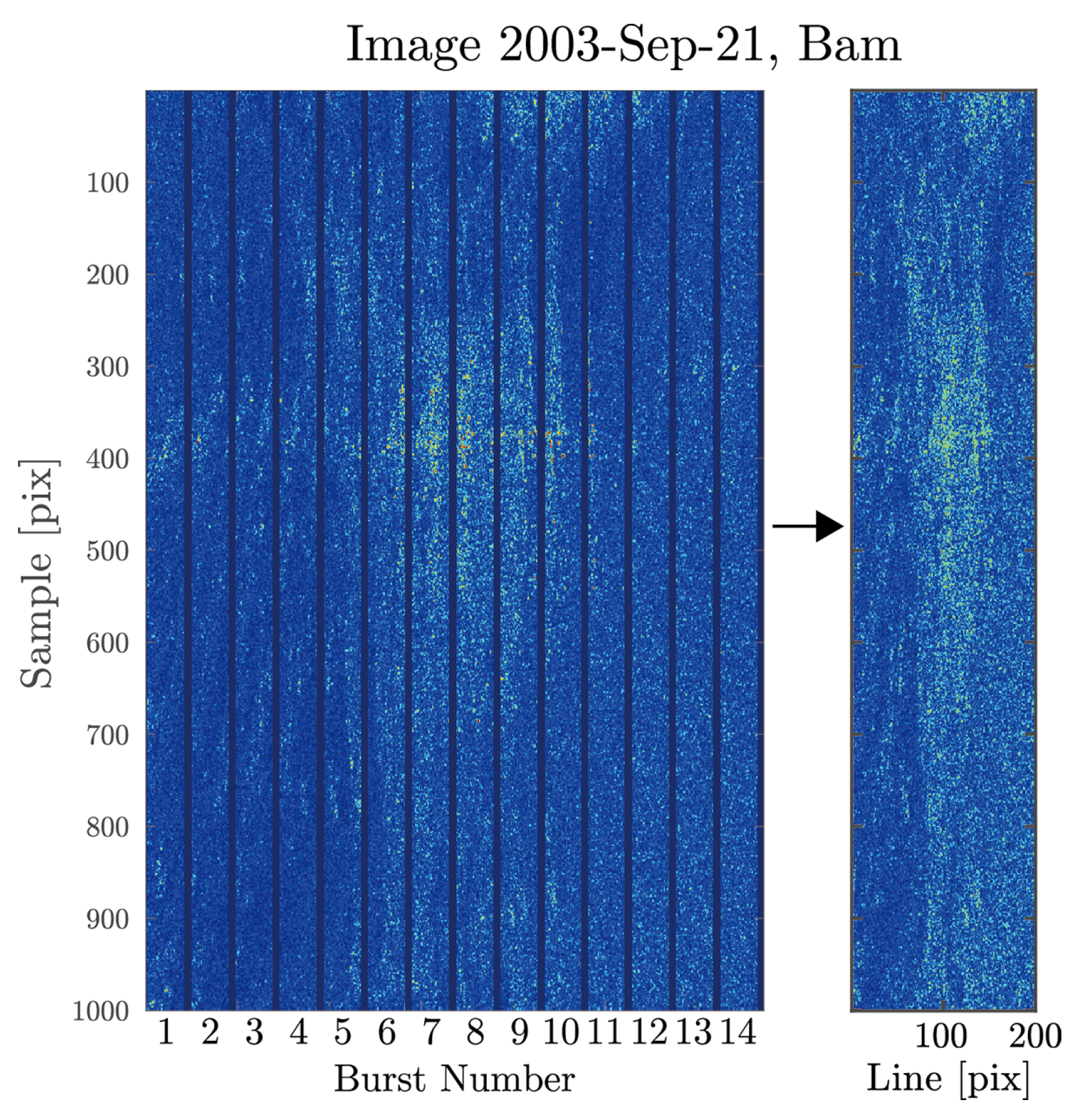
In addition, there have been several studies on ScanSAR interferometry. To summarize, there are mainly two ways to focus ScanSAR image for the interferometric purpose. The first one is the “full-aperture focusing” [28]. The output SLCs of this focusing algorithm are similar to the stripmap (in the sense that the SLC is continuous in azimuth and there are no individual bursts) and could be used directly in the stripmap interferometric processing chain. Currently, ALOS-2 releases SLCs focused from the full-aperture algorithm [29]. The second method, called the burst-by-burst focusing method, is considered as the more standard approach. There are a few ways to focus burst-by-burst [4,30,31], but they all deliver the burst mode SLCs. More discussions on the two focus approaches could be found in [22,32]. In our work, we will mainly work with Envisat ScanSAR SLC images delivered by ESA, which is in this burst mode [33]. An example of the burst mode SLC is given in Figure 3. Finally, it is worth mentioning the work of [34] where she studied the interferometry between ScanSAR and stripmap. In her work, she worked with burst mode ScanSAR SLC images. She focused the stripmap mode raw data by only extracting the spectrum that corresponds to the bursts in ScanSAR, so that a “ScanSAR-like” image is focused from stripmap raw data so that one can do stripmap-ScanSAR interferometry. In conclusion, most of the previous studies on ScanSAR interferometry were about different focus methods for ScanSAR and the interferometry between ScanSAR and stripmap (Note that, in the TOPS mode, due to the squint angle in azimuth, there would not be any azimuth common bandwidth with respect to the stripmap mode except for the very few lines in the middle of burst where the squint angle is close to zero, thus it is not possible to do TOPS-stripmap interferometry).
Compared with previous studies that showed similar ideas, this study will focus more on the technical details in the following aspects:
- Designing the user-friendly “stripmap-like” interface for processing the wide swath mode. As mentioned above, this interface, including the processing steps and all outcomes, will be identical to processing a stripmap;
- Designing the common processing chain for ScanSAR and TOPS. Although ScanSAR and TOPS work differently in terms of imaging, a common processing chain is feasible because the two systems share a large portion of similarities and their impulse response functions (IRFs) are almost identical. Hence, the processing flow could be commonly used for both systems;
- In addition, we propose a simple method for correcting the miscoregistration residual that is estimated during the ESD step. This method does not require a resampling of the slave SLC using the conventional interpolation methods, but only requires a modulation in the frequency domain. This method will be more efficient because it only requires a point-wise multiplication in the time domain.
This article is organized as follows. Section 2 shows the burst mode nature and azimuth IRF of ScanSAR and TOPS. The reason why ScanSAR and TOPS could use the same interferometric processing chain is explained based on their IRFs. Section 3 describes the technical details behind the implementation of the common interferometric processing chain. A quick way of doing slave resampling in the ESD step is also introduced here. Section 4 briefly compares the conventional approach and the “stripmap-like” approach by using real data. Section 5 is the conclusion. Appendix A shows some interferogram examples for TOPS and ScanSAR data.
2. Burst Nature and Impulse Response Function of Wide Swath Mode
2.1. Bursts Nature and Impulse Response Function of Sentinel TOPS
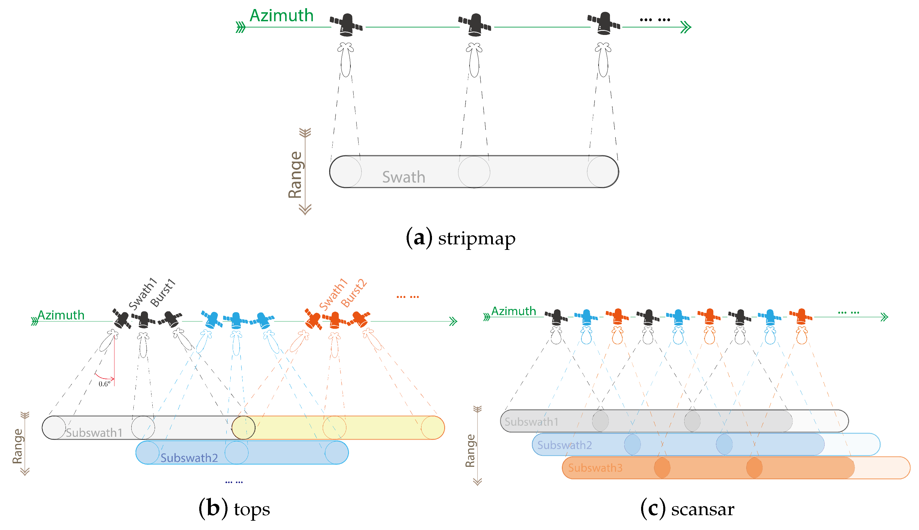
An illustration of TOPS burst mode with two subswaths is shown in Figure 4b. The satellite starts with subswath 1. By electronically steering the antenna back-to-forth along the azimuth direction, the scan covers a longer area in the same scanning duration of stripmap mode (Figure 4a). In TOPS mode, the steering angle usually goes from to in the azimuth direction. A complete antenna steering back-to-forth is called a burst. Inside one burst, the image is continuous (means the sampling grid is even). After scanning one burst in the first subswath, the antenna switches to the next subswath by adjusting the incidence angle. Upon completion, in a two-subswath system, the system will then switch back to the first subswath and scan the next burst. To make sure the final image (after stitching) is continuous and does not have any gaps, the consecutive bursts from the same subswath will have a small overlapping area. This means that every target inside the overlapping area is scanned twice from different squint angles. This overlapping area is critical for the coregistration purpose. The typical overlap is around 120 valid lines (around 2 km on the ground). TOPS burst mode trades resolution in azimuth for broader coverage in range. To scan more subswaths, the time duration for scanning each burst will decrease. Hence, the azimuth bandwidth will decrease. This will correspondingly decrease the azimuth resolution.
is the azimuth zero doppler time; is the beam center crossing time; is the azimuth envelope of compressed target and is typically a function; is the slant range of closest approach to the target; is the doppler centroid rate in the focused TOPS SLC data; is the doppler centroid frequency without introducing the steering of the antenna, and could be thought of equivalent to the doppler centroid in the stripmap case. Since TOPS is total zero doppler steered [13], is very close to zero (a measured Hz for S1).
Here, it is worth stating a few notes regarding the IRF of TOPS:
- This equation is the most important point in this article. Everything hereinafter is based on this equation: stitching, deramping, coregistration, etc. This equation is what makes TOPS different from the stripmap mode. However, the equation is really very simple, elegant and the only difference between TOPS and stripmap [37] is the last term in the equation, the quadratic phase term . The intuitive understanding of this term is the extra doppler introduced by the steering of the antenna along the azimuth.
- This extra quadratic phase term is also a legitimate measurement of the slant-range distance to the point target and it provides the real distance for the zero doppler geometry [16]. Therefore, this term needs to be preserved and can not be discarded if we want to do interferometry.
- This quadratic phase term is azimuth dependent and is responsible for the high coregistration accuracy requirement along the azimuth direction. For example, in the presence of a miscoregistration time of in the azimuth direction, the interferometric phase error would become and varies with azimuth time . A special coregistration method, enhanced spectral diversity (ESD), is required for perfect spectral alignment. In addition, this quadratic phase term exceeds the PRF. By Nyquist sampling theorem, when the bandwidth exceeds sampling rate (in complex domain), an alias occurs when resampling. To work around, the quadratic term and baseband term needs to be resampled separately. This is well known as the deramping and reramping process.
2.2. Bursts Nature and Impulse Response Function of ScanSAR
An illustration of ScanSAR with three subswaths is shown in Figure 4c. The first difference between ScanSAR and TOPS is that the antenna beam is not steered in the azimuth direction in ScanSAR mode. At the very beginning, by adjusting the nadir angle, the antenna scans the first subswath for a certain time period. During the scanning in one subswath, the sending/receiving of pulses is identical to the stripmap case. This process is colored as black in Figure 4c. Then, the satellite adjusts the nadir angle and starts to scan the second subswath for another certain time period. This process is colored as blue. Then, the third subswath, is colored in orange. After all subswaths are scanned, the satellite switches back to the first subswath and scans the second burst. This cycle continues as the satellite flies along. Similar to TOPS, the time period for scanning each burst is carefully calculated so that there is enough overlap area for stitching the bursts into a continuous SLC image. Note that it is not necessary to follow the sequence of subswath 1 to 2 to 3. For Envisat ScanSAR, there are five subswaths, and the scanning sequence is 1, 3, 5, 2, 4 and then back to 1.
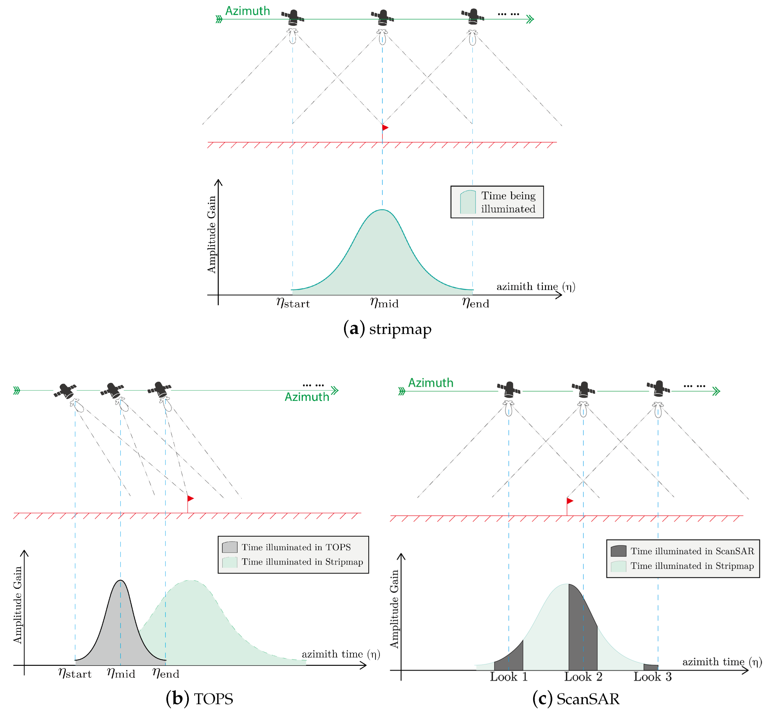
The scalloping effect of ScanSAR is explained in Figure 5. For the stripmap mode, every target on the ground is illuminated by the full antenna pattern, which has the shape shown in Figure 5a shaded in green. In ScanSAR mode, every target is only illuminated by part of the full antenna pattern because, during the other time period, the antenna is switched to other subswaths for scanning. Figure 5c shows the case of Envisat ScanSAR, where each target is illuminated three times. This means that the same target will appear in bursts 1, 2 & 3 but at different positions with different amplitude gain. This is referred to “three looks”. For the target that appears at burst edges, the received echo from the target will have the minimum gain and minimum SNR due to the roll off of amplitude envelope function. This is the scalloping effect. As a comparison, it could be seen in Figure 5b that in TOPS mode all targets are illuminated by the complete antenna beam pattern. The difference between TOPS and stripmap is that TOPS scans the target for a shorter time period and thus has a smaller azimuth bandwidth.
At last, it can be seen from Figure 5 that, in both ScanSAR and TOPS system, the beam center crossing time (time of the amplitude gain peak) is not equal to zero doppler time in general, which means that an additional doppler centroid will be introduced to their IRF in azimuth direction when comparing with stripmap.
For the ESA focused Envisat ScanSAR SLC product, the IRF on azimuth direction is [38]:
where is the azimuth frequency modulation (FM) rate. All other notations are the same as in Equation (1). Note that, In ScanSAR’s IRF, the envelope is centered at . is the mathematical expression for the scalloping effect, as we can see that the targets at burst edges will have smaller amplitude value since is usually a windowed function.
2.3. Similarities between TOPS and ScanSAR
If one compares the azimuth IRF of TOPS and ScanSAR, it could be seen that the two IRFs share much resemblance. Except for the envelope function, the only difference is that in the TOPS system the azimuth FM rate is represented as where its derivation is given in [35], but, in the ScanSAR system, the azimuth FM rate is represented by to show the distinction. The similarity determines that the processing flow for the two systems could be used interchangeably. In addition, it should be noted that the in Equation (1) and in Equation (2) are equivalent.
The three key steps for wide swath interferometric processing come naturally from the burst mode nature and IRF function. Firstly, the bursts need to be stitched into a continuous SLC image. Secondly, the quadratic phase term in IRF exceeds PRF so that deramp is required to bring the signal to baseband before resampling. Finally, as mentioned in Section 2.1, the ESD method is required for meeting the high coregistration accuracy. In the next section, the detailed processing methods will be presented.
3. The Interferometric Processing Flow
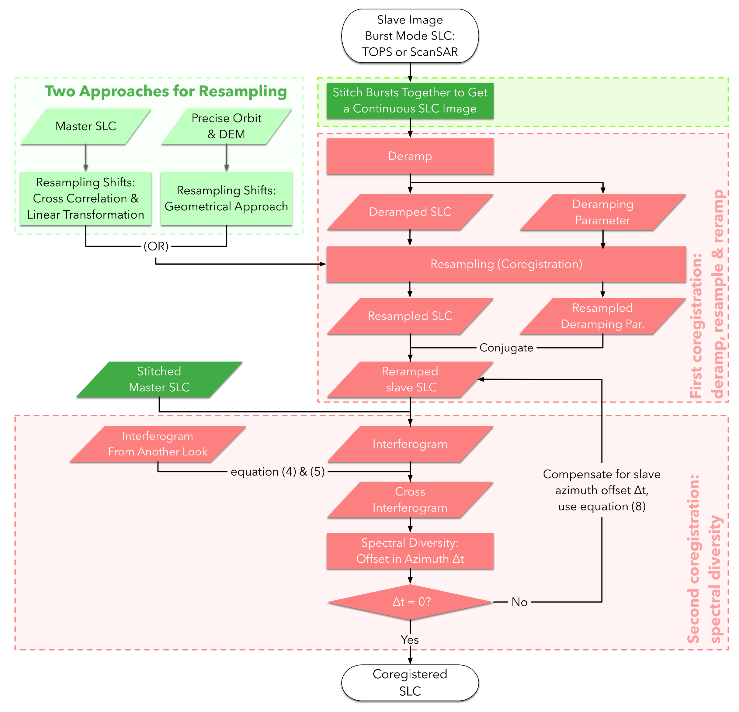
Figure 6 shows the complete proposed interferometric processing flow. In sequence, the proposed processing chain includes the following steps: (1) stitching all bursts together into a single SLC image; (2) deramping the quadratic phase of each burst; (3) conducting the initial coregistration either using the cross-correlation method [9] or the geometrical method [24]; (4) reramping the resampled quadratic phase back to resampled (coregistered) slave image; (5) conducting the fine coregistration using the enhanced spectral diversity method and compensating for the miscoregistration that is estimated by ESD; and (6) generating the interferogram. Some of the standard process details could also be found in [18]. The interferometric processing chain for ScanSAR is identical to the TOPS case. In this section, we will address some key steps, issues and new implementations in our approach.
3.1. Stitching Bursts
3.1.1. TOPS
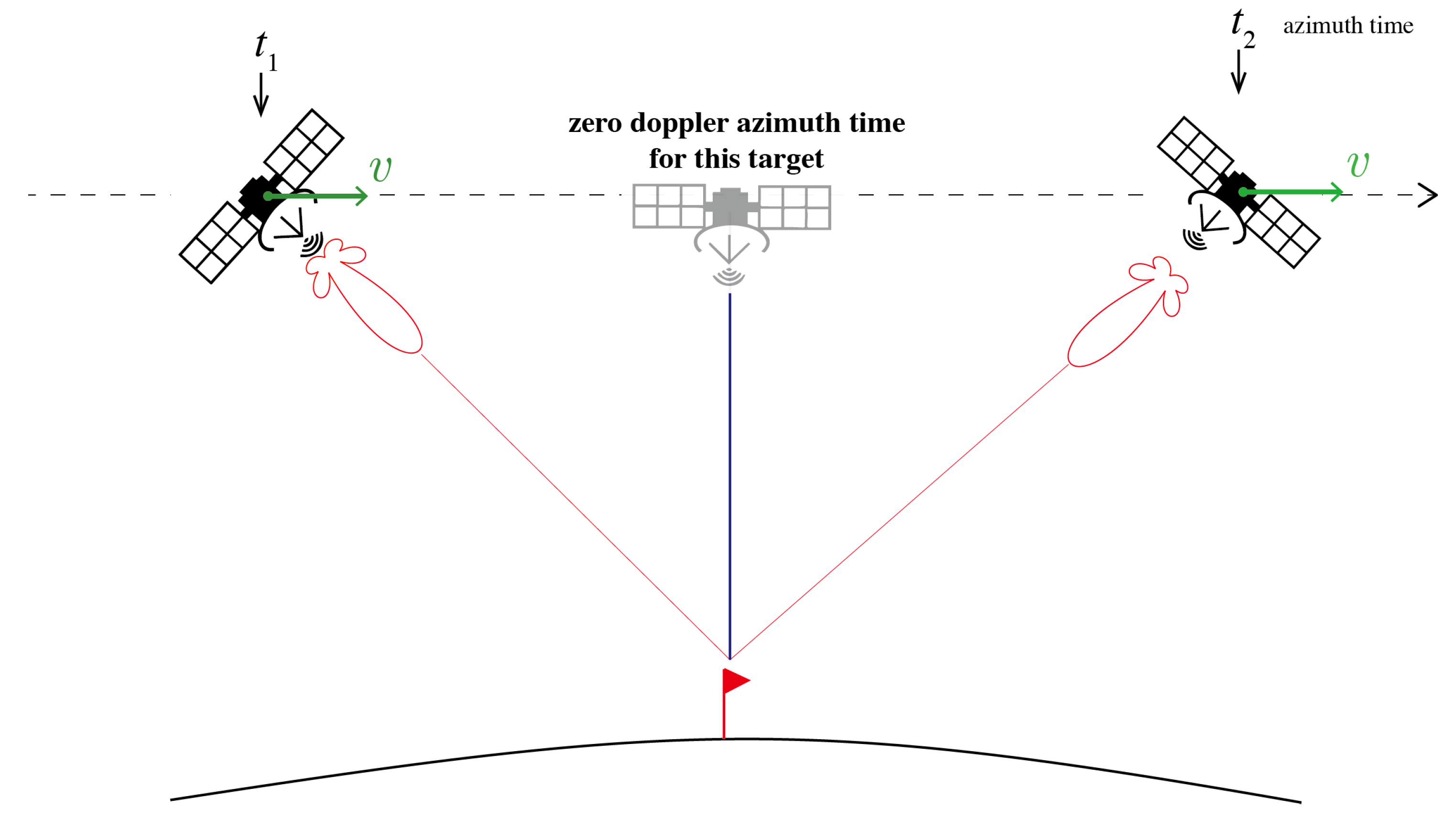
As shown in Figure 4b, there is always an overlapping area between adjacent bursts so that one could stitch them together seamlessly. The idea is simple. The zero doppler azimuth time tag for each line is used for stitching. As shown in Figure 7, take one target standing inside the bursts overlapping area as an example. The target would be illuminated twice at time and . However, the zero doppler azimuth time for this given target is unique because the zero doppler position of the satellite with respect to the target is unique. Sentinel-1 SLC is focused to zero doppler azimuth time and this time tag is written for every target. The zero doppler time tag could be used to identify the same target in burst one and burst two. The stitching is done accordingly.
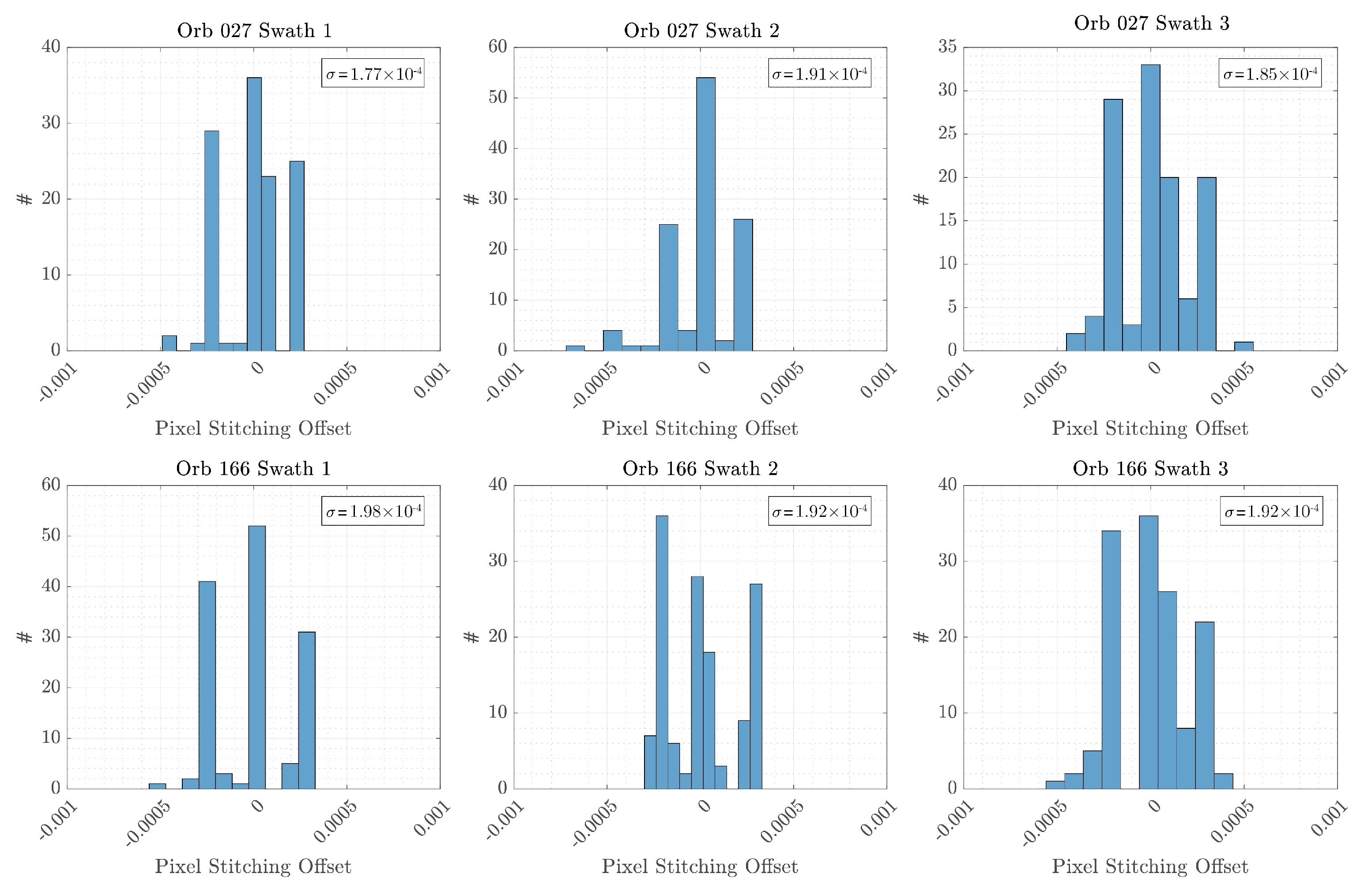
Another thing to make sure is the following: for the target shown in Figure 7, there will be two time-tags written for this target, recorded separately in burst 1 and burst 2. It is important to make sure that the two time tags have negligible difference during the SLC formation process. Since TOPS coregistration requires a 0.001 pulse repetition interval (PRI) coregistration accuracy [18], the time tag difference should be much smaller to avoid introducing extra error during the ESD steps. For validating purposes, we take one slice of S1A that consists of 117 bursts and one slice of S1B that consists of 135 bursts. The time difference in the unit of PRI for the same target in burst i and are plotted as histograms and shown in Figure 8. The result shows that the variations are all within PRI, one-fifth of 0.001 PRI. An accurate regular sampling space means that after stitching the sampling space remains a constant and no further resampling is needed. As a matter of fact, in the early experimental stage of S1A, it has been reported that [39] the time difference for stitching can be as high as 0.01 pixels, which means a resampling process is needed when stitching so that all pixels are in a common sampling grid. The issue was reported to be resolved by ESA later on.
Finally, due to Sentinel’s burst nature, concatenating more than one consecutive SLC in the azimuth direction for the same subswath is the same as stitching the bursts. The way that most SLCs delivered by ESA consist of nine bursts per subswath is merely a human-made rule. It is a trivial step to stitch consecutive SLCs in the azimuth direction.
3.1.2. ScanSAR
A typical ScanSAR burst is much shorter than TOPS burst. For example, one burst in Envisat ScanSAR consists of 48 lines. In the metadata, the zero doppler azimuth time for each line is used for stitching together the bursts using the method described in Section 3.1. Envisat ScanSAR SLC distributed by ESA is three looked. Multilooks in the ScanSAR system is the guarantee to a continuous SLC when stitching. Theoretically, a three-look system with 48 lines means that one could stitch the SLC using either the first 16 lines, the middle 16 lines or the last 16 lines. However, different from the case of TOPS, where one can stitch using either look, it is suggested to always use the middle 16 lines for stitching purposes. In the first place, due to the scalloping effect, the lines in the middle have the highest SNR and the lines at the edge have the lowest SNR. For interferometric purposes, it is proposed to select the lines with higher SNR and hence higher coherence; in the second place, there are always a few lines at the very edge with zero value. For Envisat ScanSAR, approximately 8 out of the 48 lines are zero-padded data so that the size of bursts are consistent. If one stitches using the first or last 16 lines, then the lines with zeros will show up in the stitched SLC.
3.2. Deramp
3.2.1. TOPS
The deramping step comes directly from the IRF (Equation (1)). Again, TOPS is total zero doppler steered, which means, in Equation (1), is close to zero and is also range independent (in reality, still varies in range, but the variation is very small and could be considered negligible [35]). The azimuth bandwidth without the quadratic term for TOPS is around 313 Hz and the PRF is approximately 486 Hz. However, with around 1750 Hz/s and taking 1.35 s maximum, the maximum bandwidth for the quadratic term is around 3200 Hz, almost seven times the sampling rate. According to Nyquist theorem, resampling Equation (1) directly will alias the signal. The solution is to separate the quadratic phase term from the baseband signal, resample them separately, and put them together afterward. A comprehensive instruction on deramping is given in [35].
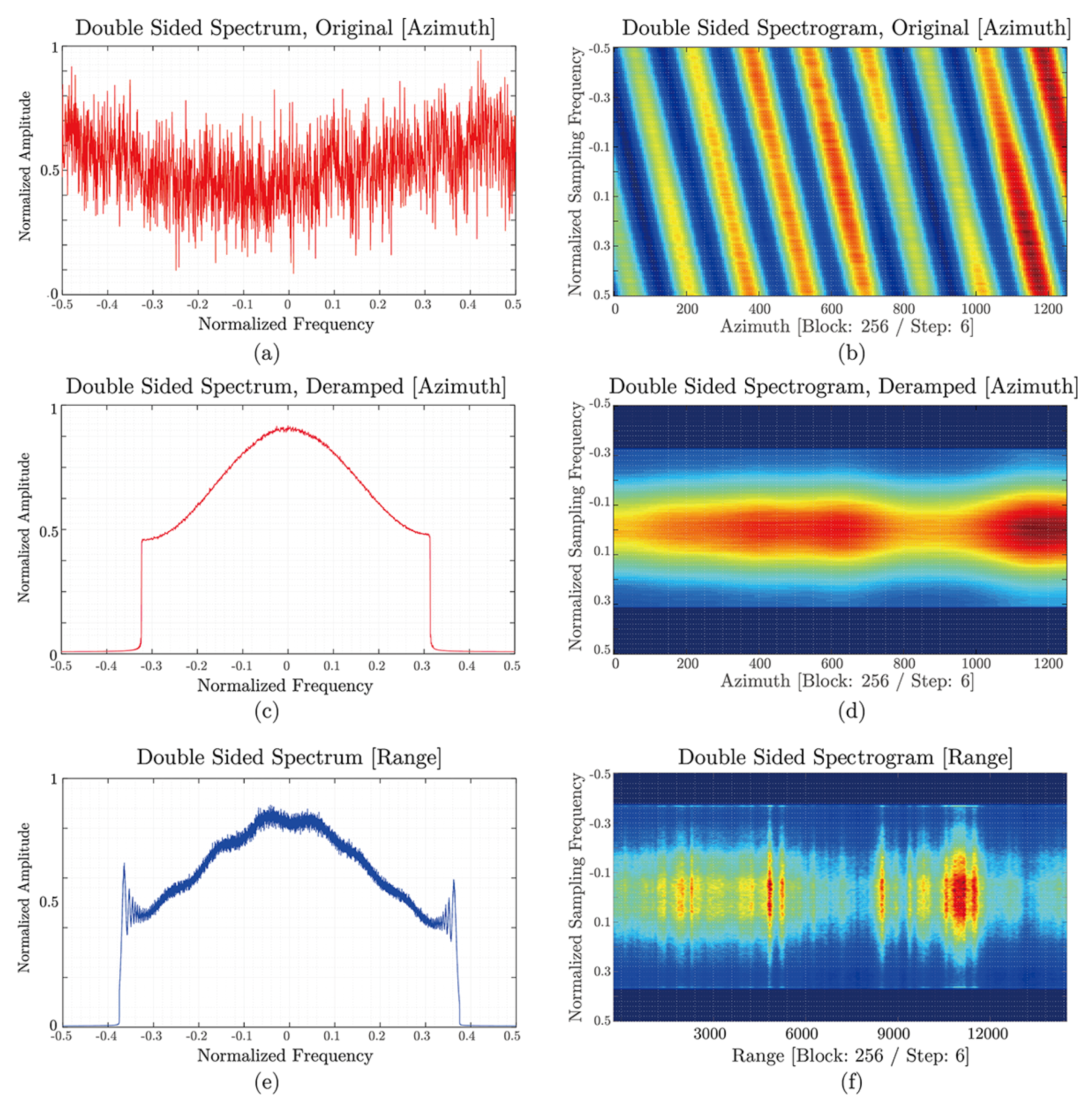
A plot of the spectrum before and after the deramping process is shown in Figure 9. To emphasize the azimuth-dependent quadratic phase before deramping, the spectrogram is also plotted in the azimuth direction. A linear variation in azimuth direction in the frequency domain could be observed. By Equation (1), one should know that the slope in Figure 9b is equal to . After deramping, two things happen: (1) the spectrum does not vary in azimuth anymore; and (2) the spectrum is limited to within PRF. At this point, the deramped slave image could be resampled aliasing-free.
There are two trivial things regarding this topic:
- TOPS is zero doppler steered, and is very close to zero. For the resampling process, it is not necessary to demodulate azimuth frequency to baseband, since the PRF (486 Hz) of TOPS system left enough margin in azimuth bandwidth (313 Hz). However, when one is using S1A or S1B data from their commissioning phase (S1A is before September 2014, S1B is before September 2016), it has been reported that the doppler centroid frequency could exceed 100 Hz [13,40]. In such cases, it is advised to also demodulate to baseband before the resampling process.
- Figure 9e,f shows that the range spectrum is baseband. This means that no extra care needs to be taken during the resampling process on the range direction.
3.2.2. ScanSAR
Again, to comply with the Nyquist sampling theorem, ScanSAR IRF needs to be deramped to baseband before doing the resampling process in coregistration. Note that, since Envisat ScanSAR system is not total zero-doppler steered, for resampling purposes, one needs to remove both the quadratic phase and the linear modulation phase when deramping. Figure 10 shows the deramping and demodulation process of a sample burst from the same data in Figure 3. Figure 10a,c is the azimuth spectrogram and spectrum before deramping. The azimuth bandwidth is much higher than the system PRF, thus the spectrum is under-sampled and severely aliased. Figure 10b,d is after deramping. The azimuth bandwidth becomes baseband and is limited to PRF. Remember that, in the TOPS system, the PRF (486 Hz) is significantly higher than azimuth bandwidth (∼300 Hz), so that there is some tolerance if the doppler centroid is shifted by a little. Here, it can be seen in Figure 10b,d,e that the PRF is just over the azimuth bandwidth with almost no margin left. This means that one needs to know (or estimate) precisely the doppler centroid and make sure that the azimuth spectrum is totally baseband and aliasing-free before the resampling process.
3.3. Initial Coregistration and Reramping
There are in general two methods for doing the initial coregistration. The first one is the cross-correlation-and-linear-transformation method [9]. The second approach is the geometrical approach [24]. The geometrical approach is often favored by the InSAR community for processing wide swath data. There are a couple of reasons for this:
- The accuracy of the geometrical method does not depend on the size of the processing area. Thus, one can apply this coregistration method to each individual burst. On the other side, if one uses the cross-correlation-and-linear-transformation method in the coregistration step, then coregistering the stitched SLC image will have a better accuracy than applying the coregistration with respect to each individual bursts because the coregistration accuracy in general increases with the image size. Stitching the bursts together will give us a bigger image and thus a better coregistration accuracy than performing the coregistration burst by burst.
More details on the comparison between the two coregistration methods are discussed in [42]. Regarding the concerns of this article, no matter which method is to be used, the essence is to estimate the pixels’ offsets between master and slave. Then, resample the deramped slave image accordingly, which is identical to the stripmap case. For resampling the quadratic phase, only the phase part in Equation (1) is resampled. This is a real number and could be resampled without getting any alias. After the real part is resampled, it is wrapped inside the operator and multiplied to the resampled baseband signal. This step is referred to as reramping.
3.4. Enhanced Spectral Diversity and a Quick Implementation of Correcting the Coregistration Error
3.4.1. TOPS
Coregistration can be thought as an “alignment” process, where one must align pixels of master and slave images perfectly. Since the complex number can be expressed as , coregistration can be thought as aligning the amplitude and the phase of master and slave image. In the case of TOPS, there is an extra quadratic phase term. The quadratic phase term has a very high frequency, thus a higher “alignment” accuracy is required to avoid the phase error due to a misalignment. In stripmap case, however, the frequency is much lower, so that a lower coregistration accuracy is enough to avoid phase bias. In addition, there is no quadratic phase term in stripmap, so a miscoregistration in stripmap will only add a constant phase bias to the entire image. For the wide swath mode, it turns out that none of the two initial coregistration methods (cross-correlation or geometrical approach) could achieve the required coregistration accuracy due to the high-frequency term in TOPS [18], and the enhanced spectral diversity method [43] is needed.
From Equation (1), suppose now there is a miscoregistration time in the slave image, the phase difference between master and miscoregistered slave is:
For simplicity, it is assumed that in Equation (1) ( only serves as a reference time and do not change the final conclusion). is the difference of between master and slave. In Equation (3), there are two unknowns, and , but only one observation, , known as the interferogram. The system is underdetermined and there is no solution for . However, if we took another measurement. Then, there are two measurements for two unknowns and then the unique solution for could be found. In TOPS, as shown in Figure 7, the targets inside the burst overlapping area receive two measurements from two different squint angles (another equivalent terminology is “two looks”. In Figure 6, the terminology “look” is used). With the two measurements (looks), one will be able to calculate . Here, we denote as . Then, ESD will generate a so-called “cross-interferogram” by the conjugate multiplication of the two measurements:
The complex conjugate multiplication cancels out most of the terms in Equation (3). A is the amplitude envelope. If we denote the phase in Equation (4) as:
Now, it becomes an equation with one observation and one unknown. Note that could be easily read from the cross interferogram phase. Hence, the miscoregistration time is derived.
We introduce here a quick implementation of correcting the miscoregistration time without the necessity of resampling the slave image again. In the first place, note that is usually very small. Take s as an example (corresponds to 0.1 pixel misalignment, which is 100 times the required coregistration accuracy) and as 20 Hz. Then, in Equation (3), . This is a constant term for the whole image with very small values. In addition, we assume that the envelope function do not change significantly when shifting by a small amount . Taking an approximation by neglecting the last term with in Equation (3), one could have the following:
Since it is assumed that the envelope function value does not change when shifting only a small amount, they canceled out when deriving Equation (6) from Equation (3). Now, by combining Equations (6) and (5), one would have:
The last term in Equation (7) is a constant phase term for the whole burst. This term is usually very small and is only adding a constant phase to the full image. A constant phase would not have any impact on the interferogram since it is already a double-reference measurement. Thus, the equation becomes:
This equation says that ESD could be applied by simply multiplying a linear phase term as a function of azimuth time to the miscoregistered slave image. It does not involve any resampling process. Equation (8) also shows that no knowledge of the doppler centroid rate is actually required for implementation. Theoretically, this is only true if we assume that is exactly the same for the two different measurements. In reality, the variation of for two different bursts is very small, so that we could safely consider a constant value and accept this conclusion. At this point, we could conclude the complete interferometric processing flow for TOPS.
3.4.2. ScanSAR
The coregistration, reramping and ESD steps are really just replicates of TOPS case. The steps are identical to TOPS case and will not be discussed here furthermore. It is only worth mentioning that, due to the presence of the quadratic phase term that exceeds the PRF, ESD is also a must for a ScanSAR system. Figure 11 shows the interferogram with and without applying the ESD.
4. Comparison between the Conventional Method and Proposed Method with Real Data
We could see from previous discussions that the proposed approach only switched the process sequences of the conventional approach based on considerations of software compatibility, applicability and user interaction. In theory, there should be no difference between the proposed approach and the conventional approach in terms of the final interferometric product. The computing complexity is also in the same order; though we care more about the correctness of the interferogram. A validation of the correctness of the proposed approach is shown in Figure 1.
In this example, we applied both the “stripmap-like” approach and the conventional approach to a full subswath that contains nine bursts (Dataset used in this example: subswath 2, S1A_IW_SLC__1SSV_20150121T134257_20150121T134325_004270_005317_EA62, S1A_IW_SLC__1SSV_20150214T134257_20150214T134324_004620_005B16_532B). Subswath 2 covers the city of Las Vegas. The geometrical method is used as the initial coregistration method for both approaches, and the reason for this was explained in Section 3.3. Figure 1 shows the important intermediate products for both approaches. This experiment shows that the final interferograms from the two approaches are identical.
5. Conclusions
In this paper, we proposed a “stripmap-like” and user-friendly interferometric processing flow that could apply for both of the wide swath modes, TOPS and ScanSAR. Instead of a burst-wise processing chain, it is proposed to stitch the bursts into a continuous SLC image at the very beginning of the processing chain. There are mainly two benefits behind this approach. In the first place, this approach enables a more user-friendly processing interface, especially for a non-SAR-expert who only wishes to apply wide swath interferometry as a tool. In the second place, the proposed method would fit into an existing stripmap processing chain with all the TOPS related processing steps applied under the hood. Regarding the interferometric processing chain, a few key issues during the processing chain are addressed, and we demonstrated a quick implementation of TOPS fine coregistration in the enhanced spectral diversity step without the need to resample the slave image for the second time. Two interferometric examples regarding TOPS and ScanSAR are shown with this processing chain.
At last, it should be worth mentioning that the proposed processing flow and the interface are already implemented into an existing SAR/InSAR processing package, SARPROZ [44], and is open to the public users. This processing package already helped other research groups doing their own applications and provided some interesting outcomes [45,46,47,48,49,50,51].
Author Contributions
The final output of this article is the result of the collaboration of all listed authors. All of the presented work was done under the supervision of D.P., who provided continuous support, advice and valuable comments throughout this project. In addition, the proposed processing chain is integrated into the InSAR processing platform that he provided, Sarproz, and is open to the public. Y.Q. designed and implemented the basic methodology and the processing flow. J.B. tested the robustness of the processing flow with TOPS and ScanSAR datasets.
Funding
This research received no external funding.
Acknowledgments
The Sentinel-1 TOPS and Envisat ScanSAR data used in this project are provided by the European Space Agency. This work is partially supported by Purdue University, West Lafayette, IN, USA and Northwestern Polytechnical University, Xi’an, China. The authors would like to thank the reviewers for their valuable comments and suggestions for this manuscript. The authors would like to thank the editors for their earnest support during the reviewing process.
Conflicts of Interest
The authors declare no conflict of interest.
Appendix A. TOPS Interferogram Examples
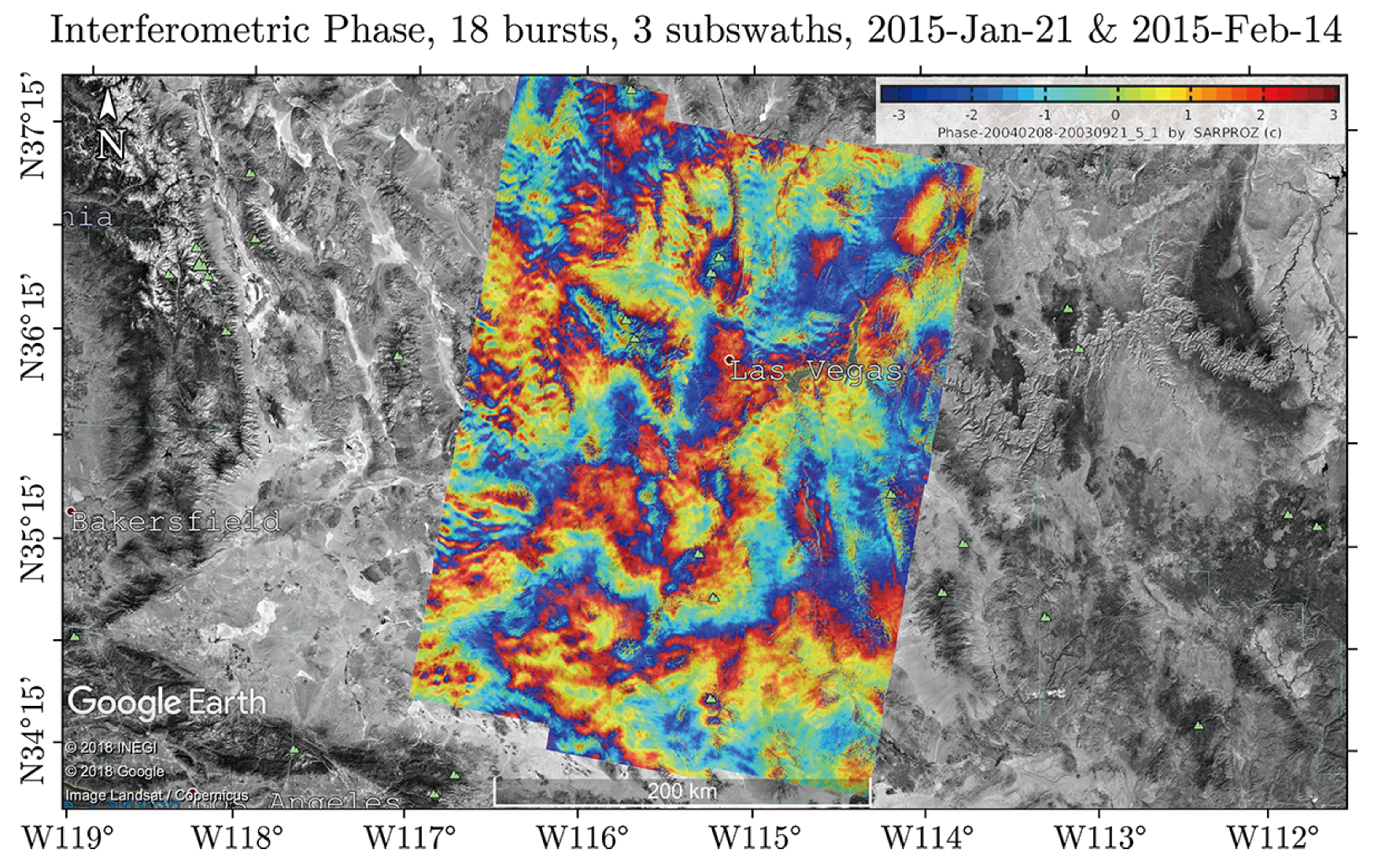
In this section, two “classic” examples of TOPS interferograms are shown. The first interferogram presented in Figure A1 is between a pair of images that comes from the early phases of S1A in January and February of 2015 (Dataset used in this example: S1A_IW_SLC__1SSV_20150121T134257_20150121T134325_004270_005317_EA62, S1A_IW_SLC__1SS V_20150214T134257_20150214T134324_004620_005B16_532B, S1A_IW_SLC__1SSV_20150121T134322_20150121T134349_004270_005317_6A6E, S1A_IW_SLC__1SSV_20150214T134322_20150214T134349_004620_005B16_3245). The area of interest (AOI) is Las Vegas and the Mojave desert in Nevada, USA. The desert area usually means a very high coherence. High coherence means that the dataset is the best candidate for testing the interferometric processing flow. The same dataset is also presented by [27]. The results from the reference and here are identical.
Figure A1.
Interferogram of the Mojave desert and Las Vegas. The interferogram consists of two full SLCs with three subswaths each. This area is an ideal site for interferometric purposes due to its high coherence.
Figure A1.
Interferogram of the Mojave desert and Las Vegas. The interferogram consists of two full SLCs with three subswaths each. This area is an ideal site for interferometric purposes due to its high coherence.

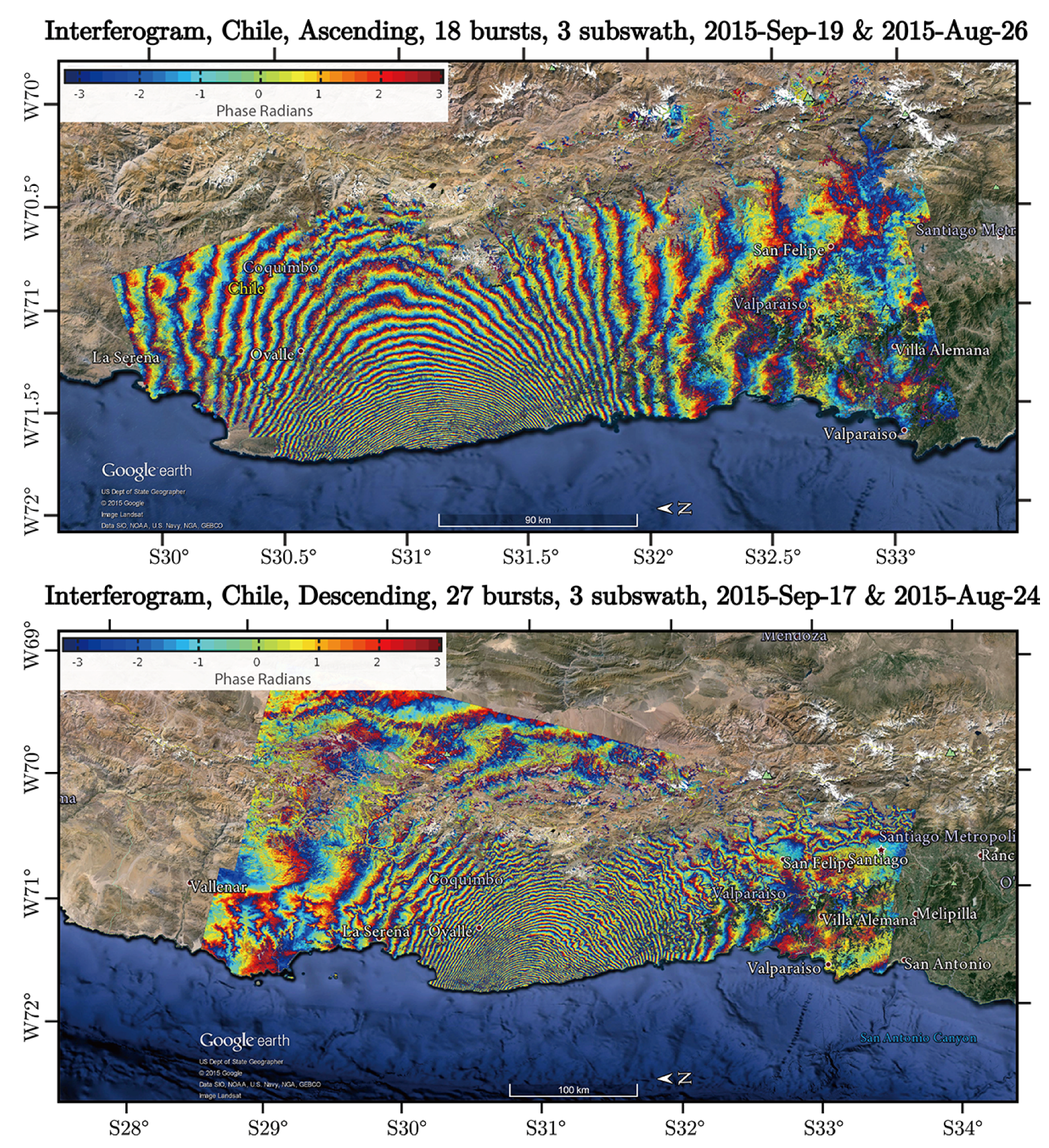
The second example shown in Figure A2 is a very good demonstration of TOPS’s capability of large area monitoring, which is exactly what TOPS is designed and served for. On 16 September, 2015, an earthquake with magnitude 8.3 hit offshore near Illapel, Chile. The huge impact of this major earthquake affected at least an area of 80000 , and the Argentina capital city Buenos Aires 1110 km away from the epic center could feel the shake. In such cases, TOPS provided images from both ascending and descending tracks. By concatenating a couple of SLCs, one can understand the full picture of this major earthquake and response promptly. Figure A2 presents two interferograms from two different tracks. The epic center of the earthquake could be quickly located at the center of the fringes, and, by counting the number of fringes, one could quickly understand the magnitude of the earthquake. Dozens of studies have been carried out for this earthquake using the Sentinel dataset.
Figure A2.
The interferograms for the 2015 Illapel earthquake happened on 16 September in Chile with a magnitude of 8.3. Upper image: interferogram from ascending track, concatenating two SLCs. Lower image: interferogram from descending track, concatenating three SLCs.
Figure A2.
The interferograms for the 2015 Illapel earthquake happened on 16 September in Chile with a magnitude of 8.3. Upper image: interferogram from ascending track, concatenating two SLCs. Lower image: interferogram from descending track, concatenating three SLCs.

Appendix B. ScanSAR Interferogram Example
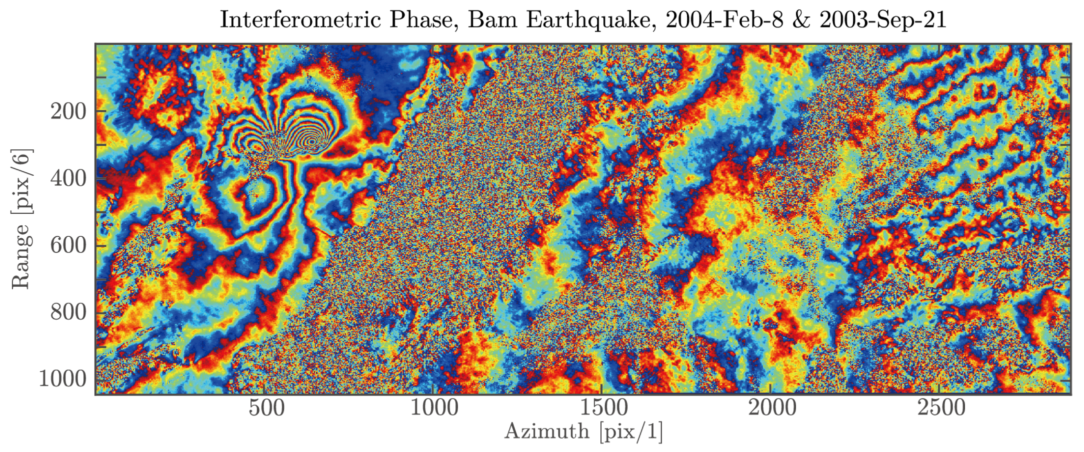
In this section, one pair of ScanSAR interferometric products is processed after implementing the ScanSAR processing chain (Dataset used in this example: ASA_WSS_1PXPDE20030921_060659_000000602020_00077_08147_0003, ASA_WSS_1PXPDE20040208_060718_000000492024_00077_10151_0004). The fringe is shown in Figure A3 and it records the Bam earthquake that happened on 26 December 2003 with magnitude 6.6. The master and slave images are taken on 21 September 2003 and 8th February 2004, respectively. Despite the half-a-year-time-interval, a good burst synchronization (91% [52]), a small normal baseline (137 m) and the fact that the AOI is located in a deserted area, all reduced other decorrelation factors. The interferogram is multilooked by 6 in the range direction so that the resolution in two directions are similar. The azimuth resolution is 80 m. The earthquake pattern is explicitly revealed by the interferogram. Note that there is a noisy line at around 1600 azimuth pixels on this interferogram. This is because a full burst is totally decorrelated in the SLC we got from ESA, which results in 18 totally noisy lines (after the stitching) on the interferogram.
Figure A3.
Interferogram of a pair of Envisat ScanSAR images showing the Bam earthquake that happened on 26 December 2003. The example contains a full subswath.
Figure A3.
Interferogram of a pair of Envisat ScanSAR images showing the Bam earthquake that happened on 26 December 2003. The example contains a full subswath.

References
- Cumming, I.G.; Wong, F.H. Chapter 4: Synthetic Aperture Concepts. In Digital Processing of Synthetic Aperture Radar Data: Algorithms and Implementation; Artech House: Norwood, MA, USA, 2005; p. 136. [Google Scholar]
- Tomiyasu, K. Conceptual performance of a satellite borne, wide swath synthetic aperture radar. IEEE Trans. Geosci. Remote Sens. 1981, GE-19, 108–116. [Google Scholar] [CrossRef]
- Moore, R.K.; Claassen, J.P.; Lin, Y.H. Scanning spaceborne synthetic aperture radar with integrated radiometer. IEEE Trans. Aerosp. Electron. Syst. 1981, AES-17, 410–421. [Google Scholar] [CrossRef]
- Guarnieri, A.M.; Prati, C. ScanSAR focusing and interferometry. IEEE Trans. Geosci. Remote Sens. 1996, 34, 1029–1038. [Google Scholar] [CrossRef]
- Holzner, J.; Bamler, R. Burst-mode and ScanSAR interferometry. IEEE Trans. Geosci. Remote Sens. 2002, 40, 1917–1934. [Google Scholar] [CrossRef]
- Farr, T.G.; Rosen, P.A.; Caro, E.; Crippen, R.; Duren, R.; Hensley, S.; Kobrick, M.; Paller, M.; Rodriguez, E.; Roth, L.; et al. The Shuttle Radar Topography mission. Rev. Geophys. 2007, 45. [Google Scholar] [CrossRef]
- Guccione, P. Interferometry with ENVISAT wide swath ScanSAR data. IEEE Geosci. Remote Sens. Lett. 2006, 3, 377–381. [Google Scholar] [CrossRef]
- Miranda, N.; Meadows, P. ASAR Wide Swath Burst Synchronization Data Update; Techreport; ESA: Paris, France, 2013. [Google Scholar]
- Ferretti, A.; Monti Guarnieri, A.; Prati, C.; Rocca, F. InSAR processing: a practical approach. In InSAR Principles: Guidelines for SAR Interferometry Processing and Interpretation; ESA: Paris, France, 2007. [Google Scholar]
- De Zan, F.; Guarnieri, A.M.M. TOPSAR: Terrain observation by progressive scans. IEEE Trans. Geosci. Remote Sens. 2006, 44, 2352–2360. [Google Scholar] [CrossRef]
- Meta, A.; Mittermayer, J.; Prats, P.; Scheiber, R.; Steinbrecher, U. TOPS imaging with TerraSAR-X: Mode design and performance analysis. IEEE Trans. Geosci. Remote Sens. 2010, 48, 759–769. [Google Scholar] [CrossRef] [Green Version]
- Wollstadt, S.; Prats, P.; Bachmann, M.; Mittermayer, J.; Scheiber, R. Scalloping correction in TOPS imaging mode SAR data. IEEE Geosci. Remote Sens. Lett. 2012, 9, 614–618. [Google Scholar] [CrossRef]
- Miranda, N.; Meadows, P.; Hajduch, G.; Pilgrim, A.; Piantanida, R.; Giudici, D.; Small, D.; Schubert, A.; Husson, R.; Vincent, P.; et al. The Sentinel-1A instrument and operational product performance status. In Proceedings of the 2015 IEEE International Geoscience and Remote Sensing Symposium (IGARSS), Milan, Italy, 26–31 July 2015; pp. 2824–2827. [Google Scholar] [CrossRef]
- Prats-Iraola, P.; Scheiber, R.; Marotti, L.; Wollstadt, S.; Reigber, A. TOPS interferometry with TerraSAR-X. IEEE Trans. Geosci. Remote Sens. 2012, 50, 3179–3188. [Google Scholar] [CrossRef] [Green Version]
- Scheiber, R.; Jäger, M.; Prats-Iraola, P.; De Zan, F.; Geudtner, D. Speckle tracking and interferometric processing of TerraSAR-X TOPS data for mapping nonstationary scenarios. IEEE J. Sel. Top. Appl. Earth Obs. Remote Sens. 2015, 8, 1709–1720. [Google Scholar] [CrossRef]
- De Zan, F.; Prats-Iraola, P.; Scheiber, R.; Rucci, A. Interferometry with TOPS: Coregistration and azimuth shifts. In Proceedings of the 10th European Conference on Synthetic Aperture Radar (EUSAR 2014), Berlin, Germany, 3–5 June 2014; pp. 1–4. [Google Scholar]
- Potin, P.; Rosich, B.; Grimont, P.; Miranda, N.; Shurmer, I.; O’Connell, A.; Torres, R.; Krassenburg, M. Sentinel-1 mission status. In Proceedings of the EUSAR 2016: 11th European Conference on Synthetic Aperture Radar, Fort Worth, TX, USA, 23–28 July 2017; pp. 1–6. [Google Scholar]
- Yagüe-Martínez, N.; Prats-Iraola, P.; González, F.R.; Brcic, R.; Shau, R.; Geudtner, D.; Eineder, M.; Bamler, R. Interferometric Processing of Sentinel-1 TOPS Data. IEEE Trans. Geosci. Remote Sens. 2016, 54, 2220–2234. [Google Scholar] [CrossRef]
- Wright, T.J.; Biggs, J.; Crippa, P.; Ebmeier, S.K.; Elliott, J.; Gonzalez, P.; Hooper, A.; Larsen, Y.; Li, Z.; Marinkovic, P.; et al. Towards Routine Monitoring of Tectonic and Volcanic Deformation with Sentinel-1. In Proceedings of the ESA FRINGE Workshop, Frascati, Italy, 23–27 March 2015. [Google Scholar]
- Geudtner, D.; Torres, R.; Snoeij, P.; Davidson, M. Sentinel-1 System Overview. In Proceedings of the ESA FRINGE Workshop, Frascati, Italy, 19–23 September 2011; pp. 1–6. [Google Scholar]
- Holzner, J. Signal Theory and Processing for Burst-Mode and ScanSAR Interferometry. Ph.D. Thesis, The University of Edinburgh, Edinburgh, UK, 2003. [Google Scholar]
- Liang, C. Interferometric Processing of Multi-Mode Synthetic Aperture Radar Data and the Applications. Ph.D. Thesis, Peking University, Beijing, China, 2014. [Google Scholar]
- Veci, L. Sentinel-1 Toolbox: TOPS Interferometry Tutorial; Techreport; ESA: Paris, France, 2016. [Google Scholar]
- Sansosti, E.; Berardino, P.; Manunta, M.; Serafino, F.; Fornaro, G. Geometrical SAR image registration. IEEE Trans. Geosci. Remote Sens. 2006, 44, 2861–2870. [Google Scholar] [CrossRef]
- Wegnüller, U.; Werner, C.; Strozzi, T.; Wiesmann, A.; Frey, O.; Santoro, M. Sentinel-1 Support in the GAMMA Software. Procedia Comput. Sci. 2016, 100, 1305–1312. [Google Scholar] [CrossRef]
- Wang, K.; Xu, X.; Fialko, Y. Improving Burst Alignment in TOPS Interferometry with Bivariate Enhanced Spectral Diversity. IEEE Geosci. Remote Sens. Lett. 2017, 14, 2423–2427. [Google Scholar] [CrossRef]
- Grandin, R. Interferometric processing of SLC Sentinel-1 TOPS data. In Proceedings of the ESA FRINGE Workshop, Frascati, Italy, 23–27 March 2015. [Google Scholar]
- Bamler, R.; Eineder, M. ScanSAR processing using standard high precision SAR algorithms. IEEE Trans. Geosci. Remote Sens. 1996, 34, 212–218. [Google Scholar] [CrossRef]
- Liang, C.; Fielding, E.J. Interferometry with ALOS-2 full-aperture ScanSAR data. IEEE Trans. Geosci. Remote Sens. 2017, 55, 2739–2750. [Google Scholar] [CrossRef]
- Sack, M.; Ito, M.R.; Cumming, I.G. Application of efficient linear FM matched filtering algorithms to synthetic aperture radar processing. In IEE Proceedings F (Communications, Radar and Signal Processing); Institution of Engineering and Technology (IET): Stevenage, UK, 1985; Volume 132, pp. 45–57. [Google Scholar]
- Moreira, A.; Mittermayer, J.; Scheiber, R. Extended chirp scaling algorithm for air-and spaceborne SAR data processing in stripmap and ScanSAR imaging modes. IEEE Trans. Geosci. Remote Sens. 1996, 34, 1123–1136. [Google Scholar] [CrossRef]
- Ortiz, A.B. ScanSAR-to-Stripmap Interferometric Observations of Hawaii. Ph.D. Thesis, Stanford University, Stanford, CA, USA, 2007. [Google Scholar]
- Kult, A.; Barstow, R.; Ramsbottom, D.; Peake, G.; Wong, T. Volume 8: ASAR Products Specifications; Techreport; ESA & MDA: Paris, France, 2016. [Google Scholar]
- Ortiz, A.B.; Zebker, H. ScanSAR-to-stripmap mode interferometry processing using ENVISAT/ASAR data. IEEE Trans. Geosci. Remote Sens. 2007, 45, 3468–3480. [Google Scholar] [CrossRef]
- Miranda, N. Definition of the TOPS SLC Deramping Function for Products Generated by the S-1 IPF; Techreport COPE-GSEG-EOPG-TN-14-0025; ESA: Paris, France, 2015. [Google Scholar]
- Piantanida, R.; Hajduch, G.; Poullaouec, J. Sentinel-1 Level 1 Detailed Algorithm Definition; Techreport SEN-TN-52-7445; ESA: Paris, France, 2016. [Google Scholar]
- Cumming, I.G.; Wong, F.H. Chapter 6: The Range Doppler Algorithin. In Digital Processing of Synthetic Aperture Radar Data: Algorithms and Implementation; Artech House: Norwood, MA, USA, 2005; p. 245. [Google Scholar]
- Cumming, I.G.; Wong, F.H. Chapter 10: Processing ScanSAR Data. In Digital Processing of Synthetic Aperture Radar Data: Algorithms and Implementation; Artech House: Norwood, MA, USA, 2005; p. 432. [Google Scholar]
- Manunta, M.; Berardino, P.; Bonano, M.; De Luca, C.; Elefante, S.; Fusco, A.; Lanari, R.; Manzo, M.; Pepe, A.; Sansosti, E.; et al. An Efficient Sentinel-1 TOPS SBAS-DInSAR Processing Chain. In Proceedings of the ESA FRINGE Workshop, Frascati, Italy, 23–27 March 2015. [Google Scholar]
- Schwerdt, M.; Schmidt, K.; Tous Ramon, N.; Klenk, P.; Yague-Martinez, N.; Prats-Iraola, P.; Zink, M.; Geudtner, D. Independent system calibration of Sentinel-1B. Remote Sens. 2017, 9, 511. [Google Scholar] [CrossRef]
- Mancon, S.; Monti Guarnieri, A.; Tebaldini, S. Sentinel-1 precise orbit calibration and validation. In Proceedings of the ESA FRINGE Workshop, Frascati, Italy, 23–27 March 2015. [Google Scholar]
- Qin, Y.; Perissin, D.; Bai, J. Investigations on the Coregistration of Sentinel-1 TOPS with the Conventional Cross-Correlation Technique. Remote Sens. 2018, 10, 1405. [Google Scholar] [CrossRef]
- Scheiber, R.; Moreira, A. Coregistration of interferometric SAR images using spectral diversity. IEEE Trans. Geosci. Remote Sens. 2000, 38, 2179–2191. [Google Scholar] [CrossRef]
- Qin, Y. Yuxiao’s Tutorials. Available online: https://www.sarproz.com/yuxiaos-tutorials/ (accessed on 1 September 2018).
- Bakon, M.; Marchamalo, M.; Qin, Y.; García-Sánchez, A.J.; Alvarez, S.; Perissin, D.; Papco, J.; Martínez, R. Madrid as Seen from Sentinel-1: Preliminary Results. Procedia Comput. Sci. 2016, 100, 1155–1162. [Google Scholar] [CrossRef]
- Canaslan Comut, F.; Ustun, A.; Lazecky, M.; Perissin, D. Capability of Detecting Rapid Subsidence with COSMO SKYMED and Sentinel-1 Dataset over Konya City. In Proceedings of the Living Planet Symposium, Prague, Czech Republic, 9–13 May 2016; ESA Special Publication: Paris, France, 2016; Volume 740, p. 295. [Google Scholar]
- Milillo, P.; Bürgmann, R.; Lundgren, P.; Salzer, J.; Perissin, D.; Fielding, E.; Biondi, F.; Milillo, G. Space Geodetic Monitoring of Engineered Structures: The Ongoing Destabilization of the Mosul Dam, Iraq. Sci. Rep. 2016, 6. [Google Scholar] [CrossRef] [PubMed]
- Lazecky, M.; Comut, F.C.; Bakon, M.; Qin, Y.; Perissin, D.; Hatton, E.; Spaans, K.; Mendez, P.J.G.; Guimaraes, P.; de Sousa, J.J.M.; et al. Concept of an Effective Sentinel-1 Satellite SAR Interferometry System. Procedia Comput. Sci. 2016, 100, 14–18. [Google Scholar] [CrossRef]
- Lazecky, M.; Canaslan Comut, F.; Qin, Y.; Perissin, D. Sentinel-1 Interferometry System in the High-Performance Computing Environment. In The Rise of Big Spatial Data; Ivan, I., Singleton, A., Horák, J., Inspektor, T., Eds.; Springer: Cham, Germany, 2017; pp. 131–139. [Google Scholar] [CrossRef]
- Mi, S.J.; Li, Y.T.; Wang, F.; Li, L.; Ge, Y.; Luo, L.; Zhang, C.L.; Chen, J.B. A Research on Monitoring Surface Deformation and Relationships with Surface Parameters in Qinghai Tibetan Plateau Permafrost. In Proceedings of the International Archives of the Photogrammetry, Remote Sensing and Spatial Information Sciences, Wuhan, China, 18–22 September 2017; pp. 629–633. [Google Scholar] [CrossRef]
- Maghsoudi, Y.; van der Meer, F.; Hecker, C.; Perissin, D.; Saepuloh, A. Using PS-InSAR to detect surface deformation in geothermal areas of West Java in Indonesia. Int. J. Appl. Earth Obs. Geoinf. 2018, 64, 386–396. [Google Scholar] [CrossRef]
- Wiesmann, A.; Werner, C.; Santoro, M.; Wegmuller, U.; Strozzi, T. ScanSAR interferometry for land use applications and terrain deformation. In Proceedings of the IEEE International Conference on Geoscience and Remote Sensing Symposium, Denver, CO, USA, 31 July–4 August 2006; pp. 3103–3106. [Google Scholar] [CrossRef]
Figure 1.
A comparison between the conventional wide swath interferometric processing flow and the proposed “stripmap-like” processing flow. The details of the dataset used in this example are explained in Section 4.
Figure 1.
A comparison between the conventional wide swath interferometric processing flow and the proposed “stripmap-like” processing flow. The details of the dataset used in this example are explained in Section 4.

Figure 2.
An example of the original burst mode image and what it looks like after the bursts are stitched together into a continuous SAR image. top: a subsection of the full SLC data that contains 1500 samples in range and five bursts. The same ground features could be observed at the edges of burst i and burst i + 1. middle: the stitched SLC image where the ground features are stitched seamlessly using the time tag. bottom: the corresponding interferogram of the stitched SLC.

Figure 3.
An example of the Envisat ScanSAR burst mode image and after the bursts are stitched together into a continuous SAR image. Left: 14 bursts of the city of Bam. Each burst is 48 lines. The system is three looked so that one target will appear in three adjacent bursts. Specifically, one target will appear at the right edge of the first burst, the middle of the second burst and the left edge of the third burst. Right: the continuous SLC image after stitching the 14 bursts together. The bright area in the center of the image is the city of Bam, Iran.

Figure 4.
(a): an illustration of stripmap working mode. Stripmap simply works in a
“scan-and-receive-line-by-line” mode; (b): a simplification of TOPS working mode with two subswaths. The antenna sweeps in the azimuth direction so that at the same time a bigger area in azimuth could be scanned when comparing with the stripmap mode. The antenna then switches to the next subswath by increasing nadir angle. For the same subswath and adjacent bursts, there is always a small portion of overlap to ensure the image could be mosaicked without any gaps. Each burst is in a different color; (c): a simplification of ScanSAR working mode with three subswaths. Here, the color is used to highlight the time period for scanning different subswaths. Similar to TOPS, bursts in the same subswath will have an overlap area to make sure a continuous SLC could be stitched. The biggest difference between ScanSAR and TOPS is that ScanSAR does not steer antenna electronically in the azimuth direction. Antenna beam pattern is only switched between subswath by adjusting the nadir angle.

Figure 5.
The illustration of the working mode for stripmap, TOPS and ScanSAR and the amplitude
gain as a function of the azimuth time for one point target on the ground. (a) is the amplitude gain of the ground target for stripmap with zero Doppler. In (b,c), the grey color represents the time period that the given target on the ground (labeled in red) is scanned under TOPS or ScanSAR modes, and the green color is the stripmap mode as a reference.

Figure 6.
The complete interferometric processing flow for TOPS and ScanSAR.

Figure 7.
Stitching bursts using the zero doppler time tag of each target.

Figure 8.
The histogram of zero doppler time difference for targets in the burst overlapping zone. A total of 117 adjacent bursts are selected for the S1A track 27 and 135 bursts for S1B track 166.
Figure 8.
The histogram of zero doppler time difference for targets in the burst overlapping zone. A total of 117 adjacent bursts are selected for the S1A track 27 and 135 bursts for S1B track 166.

Figure 9.
The spectrum and spectrogram on azimuth and range direction for one single burst of TOPS. The spectrograms are calculated in blocks of 256 pixels and steps of six pixels. The frequency labels are all normalized frequency. (a,b): frequency domain along the azimuth direction, the original data; (c,d): frequency domain along the azimuth direction, after the deramping; (e,f): frequency domain along the range direction. Range spectrum is not influenced by the deramp process in azimuth.

Figure 10.
The spectrum and spectrogram on azimuth direction for one single burst of Envisat ScanSAR. The spectrograms are calculated in blocks of 16 pixels and steps of two pixels. Upper left: the spectrogram in azimuth for one burst; Lower left: the 1D azimuth spectrum (averaged) of a burst; Upper middle: the spectrogram in azimuth after applying the deramping function; Lower middle: the 1D spectrum of the burst after deramp; Right: the 2D frequency domain plot of the deramped burst.

Figure 11.
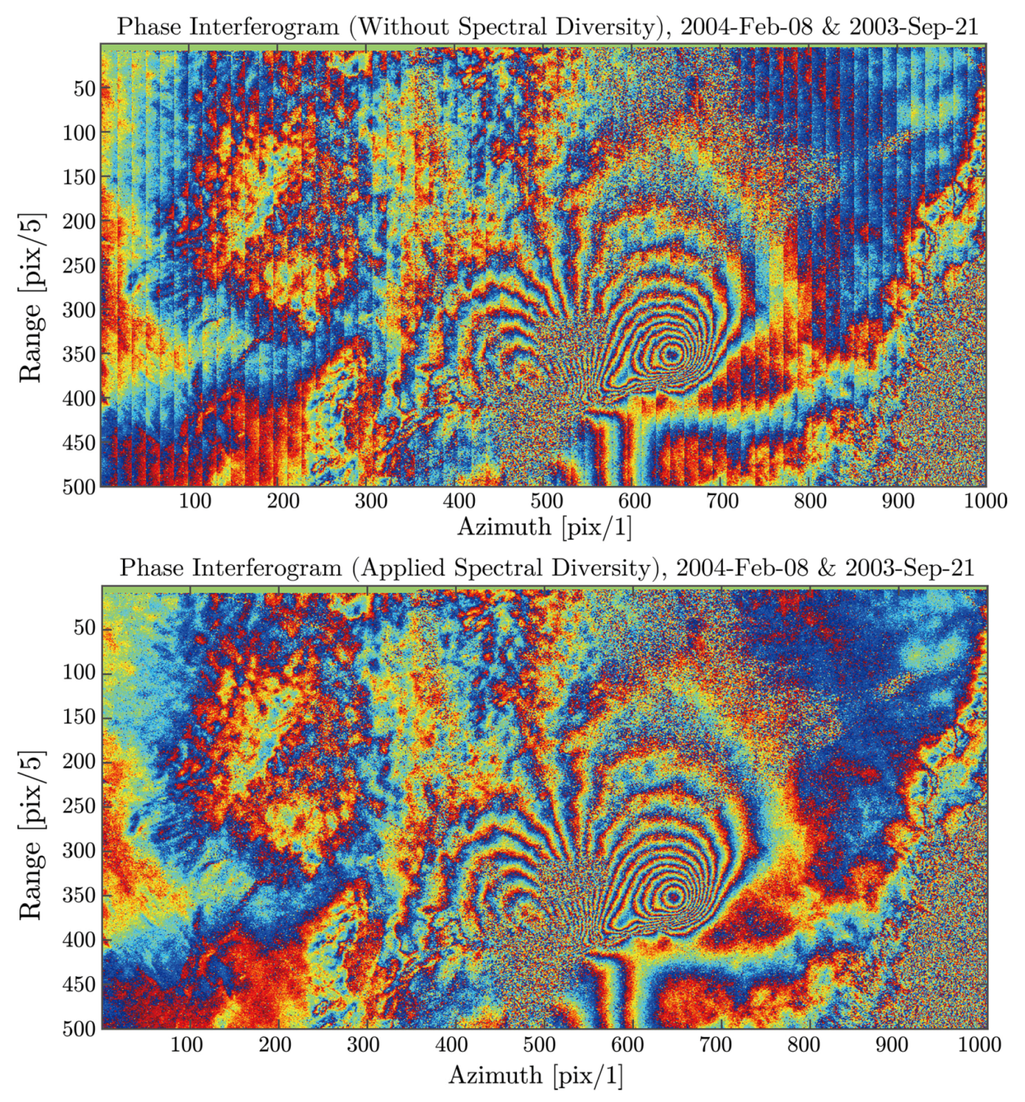
Upper: The final interferogram (multilooked by 5 in range direction) without performing the ESD correction. Lower: the interferogram after performing the ESD correction.
Figure 11.
Upper: The final interferogram (multilooked by 5 in range direction) without performing the ESD correction. Lower: the interferogram after performing the ESD correction.

© 2018 by the authors. Licensee MDPI, Basel, Switzerland. This article is an open access article distributed under the terms and conditions of the Creative Commons Attribution (CC BY) license (http://creativecommons.org/licenses/by/4.0/).
Share and Cite
MDPI and ACS Style
Qin, Y.; Perissin, D.; Bai, J. A Common “Stripmap-Like” Interferometric Processing Chain for TOPS and ScanSAR Wide Swath Mode. Remote Sens. 2018, 10, 1504. https://doi.org/10.3390/rs10101504
AMA Style
Qin Y, Perissin D, Bai J. A Common “Stripmap-Like” Interferometric Processing Chain for TOPS and ScanSAR Wide Swath Mode. Remote Sensing. 2018; 10(10):1504. https://doi.org/10.3390/rs10101504
Chicago/Turabian StyleQin, Yuxiao, Daniele Perissin, and Jing Bai. 2018. "A Common “Stripmap-Like” Interferometric Processing Chain for TOPS and ScanSAR Wide Swath Mode" Remote Sensing 10, no. 10: 1504. https://doi.org/10.3390/rs10101504
Note that from the first issue of 2016, this journal uses article numbers instead of page numbers. See further details here.