Testing of Grouped Product for the Weibull Distribution Using Neutrosophic Statistics

Aslam, Muhammad; Arif, Osama H.

doi:10.3390/sym10090403

Open AccessArticle

Testing of Grouped Product for the Weibull Distribution Using Neutrosophic Statistics

by

Muhammad Aslam

^*

and

Osama H. Arif

Department of Statistics, Faculty of Science, King Abdulaziz University, Jeddah 21589, Saudi Arabia

^*

Author to whom correspondence should be addressed.

Symmetry 2018, 10(9), 403; https://doi.org/10.3390/sym10090403

Submission received: 21 August 2018 / Revised: 5 September 2018 / Accepted: 11 September 2018 / Published: 15 September 2018

Download

Browse Figure

Versions Notes

Abstract

:

Parts manufacturers use sudden death testing to reduce the testing time of experiments. The sudden death testing plan in the literature can only be applied when all observations of failure time/parameters are crisp. In practice however, it is noted that not all measurements of continuous variables are precise. Therefore, the existing sudden death test plan can be applied if failure data/or parameters are imprecise, incomplete, and fuzzy. The classical statistics have the special case of neutrosophic statistics when there are no fuzzy observations/parameters. The neutrosophic fuzzy statistics can be applied for the testing of manufacturing parts when observations are imprecise, incomplete and fuzzy. In this paper, we will design an original neutrosophic fuzzy sudden death testing plan for the inspection/testing of the electronic product or parts manufacturing. We will assume that the lifetime of the product follows the neutrosophic fuzzy Weibull distribution. The neutrosophic fuzzy operating function will be given and used to determine the neutrosophic fuzzy plan parameters through a neutrosophic fuzzy optimization problem. The results of the proposed neutrosophic fuzzy death testing plan will be implemented with the aid of an example.

Keywords:

neutrosophic fuzzy statistics; fuzzy approach; neutrosophic fuzzy plan parameters; fuzzy optimization problem; risks

1. Introduction

In life testing experiments, a random sample of items is usually selected, and a single item is installed on a single tester for the lot sentencing. This type of testing is costly as the number of testers is equal to the number of items that are selected for the testing purpose. Alternatively, the group sampling scheme is applied for the testing of more than one item on the single tester. Sudden death testing is implemented in groups to reduce the testing/inspection cost of the product. In sudden death testing, a random sample of size

n

is equally distributed to

g

groups having

r

items in each of the

g

groups. Reference [1] proposed the sudden test for the Weibull distribution. According to Reference [1] “The specimens in each group are tested identically & simultaneously on different testers. The 1st group of specimens is run until the 1st failure occurs. At this point, the surviving specimens are suspended & removed from testing. An equal set of new specimens numbering is next tested until the 1st failure. This process is repeated until one failure is generated from each of the groups”. The sampling plan for sudden death testing has been considered by several authors in the literature, see for example References [1,2,3].

In the modern era, products are manufactured using advanced technology, which result in high quality and reliability. For the testing/inspection of a highly reliable product, it may not be possible to wait for the failures of the product for the lot sentencing. The two types of censoring widely applied to reduce the testing cost for a highly reliable product, are known as type-I censoring and type-II censoring. The testing is said to be type-I censoring if the time of experiment is fixed, and type-II if the number of failures is specified for the testing/inspection of the product. The acceptance sampling plans for type-I and type-II censoring when the lifetime follows the Weibull distribution is designed by a number of researchers, including, for example, References [4,5,6,7,8,9,10].

The fuzzy approach is widely used when there is some uncertainty in the proportion of defectives. In practice, the experimenter may be indeterminate about the percentage of defectives. In this case, the traditional sampling plans can be applied for the inspection of the lot. Hence, a number of people have designed efficient sampling plans using the fuzzy approach, including, for example, References [11,12,13,14,15,16,17,18,19,20,21,22,23,24,25,26].

Parts manufacturers use sudden death testing to reduce the testing time of the experiment. The sudden death testing plan in the literature can only be applied when all observations of failure time/parameters are crisp. According to Reference [27], “all observations and measurements of continuous variables are not precise numbers but more or less non-precise. This imprecision is different from variability and errors. Therefore, lifetime data are also not precise numbers but more or less fuzzy. The best up-to-date mathematical model for this imprecision is so-called non-precise numbers”. Therefore, the existing sudden death test plan can be applied if failure data or parameters are imprecise, incomplete, and fuzzy. The classical statistics have the special case of the neutrosophic statistics when there are no fuzzy observations/parameters. Thus, the neutrosophic fuzzy statistics can be applied for the testing of manufacturing parts when observations are imprecise, incomplete, and fuzzy. Recently, the authors of Reference [28] introduced the neutrosophic statistics in the area of acceptance sampling plan.

By exploring the literature, and to the best of the author’s knowledge, there is no work on the design of neutrosophic fuzzy sudden death testing plan using the Weibull distribution. In this paper, we will design an original neutrosophic fuzzy sudden death testing plan for the inspection/testing of the electronic product or parts manufacturing. We will assume that the lifetime of the product follows the neutrosophic fuzzy Weibull distribution. The neutrosophic fuzzy operating function will be given and used to determine the neutrosophic fuzzy plan parameters through a neutrosophic fuzzy optimization problem. The results of the proposed neutrosophic fuzzy death testing plan will be implemented with the aid of an example.

2. Design of Proposed Plan

Suppose that

T_{N i} ϵ {T_{L}, T_{U}} = i =

1, 2, 3, …,

n_{N}

being a random sample from the neutrosophic fuzzy Weibull distribution with neutrosophic fuzzy shape parameter

m_{N}

and neutrosophic fuzzy scale parameter

λ_{N}

. The neutrosophic fuzzy Weibull distribution is defined by:

F_{N} (t_{N}; m_{N}, λ_{N}) = 1 - e x p (- {(t_{N} / λ_{N})}^{m_{N}}), t_{N} \geq 0

(1)

Some more details on fuzzy based Weibull distribution can be seen in References [29,30].

It is assumed that items are tested identically and simultaneously in each group. We propose following a neutrosophic fuzzy sudden death testing plan. The quality characteristic beyond the lower specification limit

L

is defined as defective. Thus, the probability of defectiveness is given by:

p_{N} = p_{r_{N}} {T_{N} < L} = F_{N} (L)

(2)

For the given

p_{N}

, the corresponding

λ_{N} L

from Equation (2) is given by:

w_{N} = - l n (1 - p_{N}) = {(λ_{N} L)}^{m_{N}}

(3)

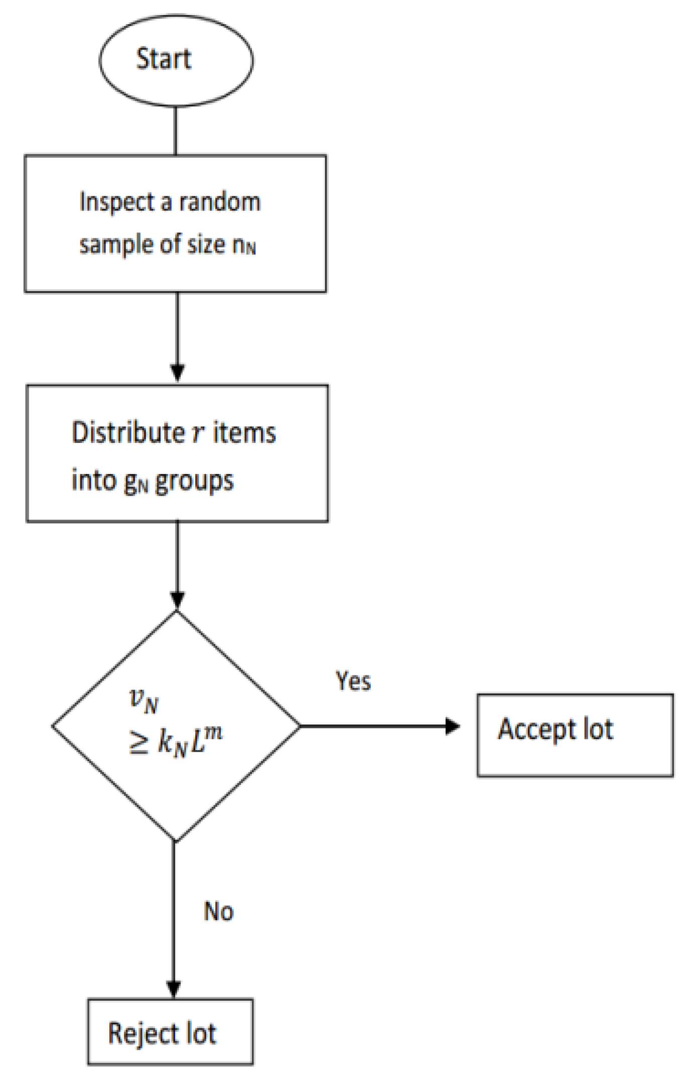
Step 1.: Select a random sample $n_{N} ϵ {n_{L}, n_{U}}$ and distribute $r$ items into $g_{N} ϵ {g_{L}, g_{U}}$ groups.
Step 2.: Record first failure from ith group $(i = 1, 2, \dots g_{N})$ and calculate neutrosophic fuzzy statistic $v_{N} = \sum_{i = 1}^{g_{N}} Y_{i N}^{m}$ ; $g_{N} ϵ {g_{L}, g_{U}}$ , $v_{N} ϵ {v_{L}, v_{U}}$ .
Step 3.: Accept lot of the product if $v_{N} \geq k_{N} L^{m}$ , $k_{N} ϵ {k_{a L}, k_{a U}}$ is a neutrosophic fuzzy acceptance number.

The proposed plan has two neutrosophic fuzzy parameters

g_{N} ϵ {g_{L}, g_{U}}

and

k_{N} ϵ {k_{a L}, k_{a U}}

. The proposed sampling plan is the extension of the plan proposed in Reference [1]. The proposed sampling plan reduces to the plan in Reference [1] when

g_{L} = g_{U} = g

and

k_{a L} = k_{a U} = k

. The operational process of the proposed plan is also shown in Figure 1.

By following Reference [1] that

Y_{i N}^{m}

in

v_{N} = \sum_{i = 1}^{g_{N}} Y_{i N}^{m}

follows the i.i.d. neutrosophic exponential distribution with neutrosophic parameter

λ_{N}^{m_{N}} r_{N}

, so

v_{N}

follows the neutrosophic fuzzy gamma distribution with neutrosophic parameters

(g_{N}, λ_{N}^{m_{N}} r_{N})

;

g_{N} ϵ {g_{L}, g_{U}}

. The neutrosophic fuzzy operating function (NFOC) will be derived as follows:

L (p_{N}) = 1 - G_{2 g_{N}} (2 r_{N} k_{N} w_{N}); k_{N} ϵ {k_{a L}, k_{a U}}

(4)

where

G_{δ_{N}}

is the neutrosophic fuzzy cumulative distribution function of the neutrosophic fuzzy gamma with a neutrosophic degree of freedom

δ_{N}

.

Neutrosophic Fuzzy Non-Linear Optimization

Let

α

and

β

respectively be the producer’s risk and consumer’s risk. The plan parameters

g_{N} ϵ {g_{L}, g_{U}}

and

k_{N} ϵ {k_{a L}, k_{a U}}

will be determined

L (C_{A Q L}) \geq 1 - α

at acceptable quality level (AQL =

p_{1}

) and

L (C_{L Q L}) \leq β

at limiting quality level (LQL =

p_{2}

). Therefore, the neutrosophic fuzzy plan parameters of the proposed plan will be determined by following the neutrosophic fuzzy non-linear optimization problem:

minimize n_{N} ϵ {n_{L}, n_{U}}

(5)

L (C_{A Q L}) = (1 - G_{2 g N} (2 r_{N} k_{N} w_{N 0})) \geq 1 - α, k_{N} ϵ {k_{L}, k_{U}}; g_{N} ϵ {g_{L}, g_{U}}

(6)

L (C_{L Q L}) = (1 - G_{2 g N} (2 r_{N} k_{N} w_{N 1})) \leq β, k_{N} ϵ {k_{L}, k_{U}}; g_{N} ϵ {g_{L}, g_{U}}

(7)

The plan parameters

g_{N} ϵ {g_{L}, g_{U}}

and

k_{N} ϵ {k_{a L}, k_{a U}}

will be determined through Equations (5)–(7) using the grid search method. The following algorithm is used to determine the plan parameters.

Step 1.: Specify the value of r.
Step 2.: Determine the values of $g_{N}$ and $k_{N}$ using the search grid method through Equations (5)–(7).
Step 3.: Choose the parameters for the plan where indeterminacy interval in $g_{N}$ is minimum.

The combinations that have smaller values of

n_{N} ϵ {n_{L}, n_{U}}

are selected and reported in Table 1 and Table 2. Table 1 reports for

g_{N} ϵ {g_{L}, g_{U}}

and

k_{N} ϵ {k_{a L}, k_{a U}}

when

r

= 5 and Table 2 reports for

g_{N} ϵ {g_{L}, g_{U}}

and

k_{N} ϵ {k_{a L}, k_{a U}}

when

r

= 10. From Table 1 and Table 2, we noted the following trend in

g_{N} ϵ {g_{L}, g_{U}}

and

k_{N} ϵ {k_{a L}, k_{a U}}

.

For the fixed values of neutrosophic parameters, $g_{N} ϵ {g_{L}, g_{U}}$ and $k_{N} ϵ {k_{a L}, k_{a U}}$ decrease as $r$ increases from 5 to 10.
For the fixed values of neutrosophic parameters, $g_{N} ϵ {g_{L}, g_{U}}$ and $k_{N} ϵ {k_{a L}, k_{a U}}$ decrease as LQL increases.

3. Application of Proposed Plan

The application of the proposed plan will be given on the ball bearing quality assurance, as the quality characteristic is measurable and as there is a chance that some observations may be fuzzy. Suppose that the ball bearing manufacturer is interested in applying the proposed sampling plan, but is not certain how to select suitable plan parameters for the testing of his product. Suppose he decides to install five items on the single tester. Let AQL = AQL = 0.001, LQL = 0.010,

α

= 0.05 and

β

= 0.10. From Table 1, we have

g_{N} ϵ {3, 5}

and

k_{N} ϵ {106.0, 160.8}

. Hence, he can select

g

between 3 and 5. Suppose experimenter decides to select a random sample size

n

= 25 and

g

= 5.

Step 1.: Select a random sample 25 and distribute five items into five groups.
Step 2.: Perform sudden death testing and note down the first failure from each of the five groups $(i = 1, 2, \dots, 5)$ . The number of first failures from the five groups are Y₁ = [220, 230], Y₂ = [300, 320], Y₃ = 285, Y₄ = [155, 165] and Y₅ = [365, 375]. The lifetime of ball bearing follows the neutrosophic Weibull distribution with parameter $m_{N} ϵ {2, 2}$ and lower specification limit $L$ = 200. The statistic $v_{N}$ is calculated as:

$v_{N} = \sum_{i = 1}^{g_{N}} Y_{i N}^{m}; g_{N} ϵ {3, 5}, v_{N} ϵ {106.0, 160.8} .$

v_{N} =

[220², 230²] + [300², 320²] + [285², 285²] + [155², 165²] + [365², 375²] = [376875, 404375]. Now

k_{N} L^{m_{N}} ϵ {4240000, 6432000}

. As

v_{N} < k_{N} L^{m_{N}}

, so reject the lot of ball bearing product.

4. Comparison Study

In this section, we will compare the efficiency of the proposed plan using the neutrosophic statistics and the sudden death sampling plan proposed in Reference [2] using the classical (crisp) statistics in terms of plan parameter

g

. For fair comparison, we will consider the same plan parameter values. By comparing Table 1 of the proposed plan with Table 1 of Reference [2] when r = 5, it can be seen that the proposed plan provides smaller values of

g

as compared to the plan in Reference [2]. For easy reference, we present the comparison in

g_{N}

between the proposed plan and Reference [2] in Table 3. For example, when AQL = 0.001 and LQL = 0.002 in Table 3, the proposed plan has a minimum value of

g

= 17 and a maximum value of

g

= 21, while the plan in [2] provides a crisp value of

g =

231. Therefore, the proposed plan needs a sample size of n = r*g between 85 and 105. By comparison, the existing plan needs a sample size of 1155 for the testing of the same lot of the product. From Table 3, we note that the proposed plan has a smaller

g_{N}

for all combinations of AQL and LQL. Therefore, the proposed plan required a smaller sample size for the inspection of the same product. Hence, less inspection cost is needed when the proposed sampling plan is implemented.

5. Concluding Remarks

In this paper, we have designed a neutrosophic fuzzy sudden death testing plan for the inspection/testing of the electronic product or parts manufacturing. The NFOC and neutrosophic fuzzy non-linear optimization problem are used to evaluate the proposed sampling plan. The proposed plan can be applied for the testing of parts when some observations or parameters are fuzzy. The proposed plan is the extension of a sudden death plan based on classical statistics. However, the proposed plan is more flexible than the plan based on classical statistics. Some tables are given and discussed with the help of a ball bearing example. The proposed plan can be applied for testing products in the automobile, aerospace and electronics industries. The proposed plan has the limitation that it can only be applied when the failure time follows the neutrosophic fuzzy Weibull distribution. The proposed plan for some other distribution can be considered as future research. The proposed sampling plan using big data can also be considered as future research.

Author Contributions

Conceived and designed the experiments, M.A.; Performed the experiments, M.A. Analyzed the data, M.A. and O.H.A.; Contributed reagents/materials/analysis tools, M.A.; Wrote the paper, M.A. and O.H.A.

Funding

This article was funded by the Deanship of Scientific Research (DSR) at King Abdulaziz University, Jeddah. The authors, therefore, acknowledge with thanks DSR technical and financial support.

Acknowledgments

The authors are deeply thankful to editor and reviewers for their valuable suggestions to improve the quality of this manuscript.

Conflicts of Interest

The authors declare no conflict of interest regarding this paper.

References

Jun, C.-H.; Balamurali, S.; Lee, S.-H. Variables sampling plans for Weibull distributed lifetimes under sudden death testing. IEEE Trans. Reliab. 2006, 55, 53–58. [Google Scholar] [CrossRef]
Aslam, M.; Azam, M.; Balamurali, S.; Jun, C.-H. A new mixed acceptance sampling plan based on sudden death testing under the Weibull distribution. J. Chin. Inst. Ind. Eng. 2012, 29, 427–433. [Google Scholar] [CrossRef]
Balamurali, S.; Subramani, J. Conditional variables double sampling plan for Weibull distributed lifetimes under sudden death testing. Bonfring Int. J. Data Min. 2012, 2, 12. [Google Scholar]
Fertig, K.; Mann, N.R. Life-test sampling plans for two-parameter Weibull populations. Technometrics 1980, 22, 165–177. [Google Scholar] [CrossRef]
Kwon, Y. A Bayesian life test sampling plan for products with Weibull lifetime distribution sold under warranty. Reliab. Eng. Syst. Saf. 1996, 53, 61–66. [Google Scholar] [CrossRef]
Balasooriya, U.; Saw, S.L.; Gadag, V. Progressively censored reliability sampling plans for the Weibull distribution. Technometrics 2000, 42, 160–167. [Google Scholar] [CrossRef]
Tse, S.-K.; Yang, C. Reliability sampling plans for the Weibull distribution under Type II progressive censoring with binomial removals. J. Appl. Stat. 2003, 30, 709–718. [Google Scholar] [CrossRef]
Chen, J.; Choy, S.; Li, K.-H. Optimal Bayesian sampling acceptance plan with random censoring. Eur. J. Oper. Res. 2004, 155, 683–694. [Google Scholar] [CrossRef]
Chen, J.; Chou, W.; Wu, H.; Zhou, H. Designing acceptance sampling schemes for life testing with mixed censoring. Nav. Res. Logist. 2004, 51, 597–612. [Google Scholar] [CrossRef]
Balasooriya, U.; Low, C.-K. Competing causes of failure and reliability tests for Weibull lifetimes under type I progressive censoring. IEEE Trans. Reliab. 2004, 53, 29–36. [Google Scholar] [CrossRef]
Kanagawa, A.; Ohta, H. A design for single sampling attribute plan based on fuzzy sets theory. Fuzzy Sets Syst. 1990, 37, 173–181. [Google Scholar] [CrossRef]
Tamaki, F.; Kanagawa, A.; Ohta, H. A fuzzy design of sampling inspection plans by attributes. Jpn. J. Fuzzy Theory Syst. 1991, 3, 211–212. [Google Scholar]
Cheng, S.-R.; Hsu, B.-M.; Shu, M.-H. Fuzzy testing and selecting better processes performance. Ind. Manag. Data Syst. 2007, 107, 862–881. [Google Scholar] [CrossRef]
Zarandi, M.F.; Alaeddini, A.; Turksen, I. A hybrid fuzzy adaptive sampling—Run rules for Shewhart control charts. Inf. Sci. 2008, 178, 1152–1170. [Google Scholar] [CrossRef]
Alaeddini, A.; Ghazanfari, M.; Nayeri, M.A. A hybrid fuzzy-statistical clustering approach for estimating the time of changes in fixed and variable sampling control charts. Inf. Sci. 2009, 179, 1769–1784. [Google Scholar] [CrossRef]
Sadeghpour Gildeh, B.; Baloui Jamkhaneh, E.; Yari, G. Acceptance single sampling plan with fuzzy parameter. Iran. J. Fuzzy Syst. 2011, 8, 47–55. [Google Scholar]
Jamkhaneh, E.B.; Sadeghpour-Gildeh, B.; Yari, G. Inspection error and its effects on single sampling plans with fuzzy parameters. Struct. Multidiscip. Optim. 2011, 43, 555–560. [Google Scholar] [CrossRef]
Turanoğlu, E.; Kaya, İ.; Kahraman, C. Fuzzy acceptance sampling and characteristic curves. Int. J. Comput. Intell. Syst. 2012, 5, 13–29. [Google Scholar] [CrossRef]
Divya, P. Quality interval acceptance single sampling plan with fuzzy parameter using poisson distribution. Int. J. Adv. Res. Technol. 2012, 1, 115–125. [Google Scholar]
Jamkhaneh, E.B.; Gildeh, B.S. Acceptance double sampling plan using fuzzy poisson distribution. World Appl. Sci. J. 2012, 16, 1578–1588. [Google Scholar]
Jamkhaneh, E.B.; Gildeh, B.S. Sequential sampling plan using fuzzy SPRT. J. Intell. Fuzzy Syst. 2013, 25, 785–791. [Google Scholar]
Venkateh, A.; Elango, S. Acceptance sampling for the influence of TRH using crisp and fuzzy gamma distribution. Aryabhatta J. Math. Inform. 2014, 6, 119–124. [Google Scholar]
Afshari, R.; Gildeh, B.S. Construction of fuzzy multiple deferred state sampling plan. In Proceedings of the 2017 Joint 17th World Congress of International Fuzzy Systems Association and 9th International Conference on Soft Computing and Intelligent Systems (IFSA-SCIS), Otsu, Japan, 27–30 June 2017; pp. 1–7. [Google Scholar]
Afshari, R.; Gildeh, B.S.; Sarmad, M. Multiple deferred state sampling plan with fuzzy parameter. Int. J. Fuzzy Syst. 2017, 20, 549–557. [Google Scholar] [CrossRef]
Elango, S.; Venkatesh, A.; Sivakumar, G. A fuzzy mathematical analysis for the effect of trh using acceptance sampling plans. Int. J. Pure Appl. Math. 2017, 117, 1–7. [Google Scholar]
Afshari, R.; Sadeghpour Gildeh, B.; Sarmad, M. Fuzzy multiple deferred state attribute sampling plan in the presence of inspection errors. J. Intell. Fuzzy Syst. 2017, 33, 503–514. [Google Scholar] [CrossRef]
Viertl, R. On reliability estimation based on fuzzy lifetime data. J. Stat. Plan. Inference 2009, 139, 1750–1755. [Google Scholar] [CrossRef]
Aslam, M. A new sampling plan using neutrosophic process loss consideration. Symmetry 2018, 10, 132. [Google Scholar] [CrossRef]
Huang, H.-Z.; Zuo, M.J.; Sun, Z.-Q. Bayesian reliability analysis for fuzzy lifetime data. Fuzzy Sets Syst. 2006, 157, 1674–1686. [Google Scholar] [CrossRef]
Pak, A.; Parham, G.A.; Saraj, M. Inference for the Weibull distribution based on fuzzy data. Rev. Colomb. Estad. 2013, 36, 337–356. [Google Scholar]

Figure 1. Operational procedure of proposed plan.

Table 1. The neutrosophic plan optimal parameters when r = 5.

p₁	p₂		$g_{N}$	$k_{N}$	$L (C_{A Q L})$	$L (C_{L Q L})$
0.001	0.002	Min	19	2473.2	0.952163	0.099984
	0.002	Max	21	2717.5	0.962712	0.095018
	0.003	Min	8	783.6	0.953490	0.099964
	0.003	Max	10	953.3	0.975800	0.095052
	0.004	Min	6	462.9	0.969175	0.099899
	0.004	Max	8	592.6	0.988845	0.095073
	0.006	Min	4	222.1	0.973434	0.099858
	0.006	Max	6	311.3	0.994680	0.095147
	0.008	Min	3	132.6	0.970167	0.099792
	0.008	Max	5	201.2	0.996239	0.095123
	0.010	Min	3	106.0	0.983213	0.099699
	0.010	Max	5	160.8	0.998555	0.095117
	0.015	Min	2	51.5	0.971999	0.099838
	0.015	Max	4	89.4	0.998831	0.095418
	0.020	Min	2	38.6	0.983592	0.099255
	0.020	Max	4	66.9	0.999599	0.095298
0.0025	0.005	Min	19	987.8	0.952444	0.099978
	0.005	Max	21	1085.3	0.962975	0.095069
	0.010	Min	6	184.6	0.969462	0.099904
	0.010	Max	8	236.3	0.988989	0.095133
	0.015	Min	4	88.5	0.973691	0.099564
	0.015	Max	6	123.9	0.994785	0.095364
	0.020	Min	3	52.7	0.983439	0.099924
	0.020	Max	5	80.0	0.996321	0.095083
	0.025	Min	3	42.1	0.983490	0.099512
	0.025	Max	5	63.8	0.998600	0.095342
	0.030	Min	2	25.6	0.958424	0.099282
	0.030	Max	4	44.4	0.997442	0.095051
	0.050	Min	2	15.2	0.984044	0.099320
	0.050	Max	4	26.3	0.999624	0.096062
0.005	0.010	Min	19	492.7	0.952885	0.099908
	0.010	Max	21	541.3	0.963371	0.095048
	0.015	Min	8	155.8	0.954335	0.099875
	0.015	Max	10	189.5	0.976377	0.095086
	0.020	Min	6	91.9	0.969849	0.099547
	0.020	Max	8	117.5	0.989243	0.095381
	0.030	Min	4	43.9	0.974240	0.099688
	0.030	Max	6	61.5	0.994931	0.095194
	0.040	Min	3	26.1	0.971200	0.099658
	0.040	Max	5	39.5	0.996491	0.096118
	0.050	Min	3	20.8	0.983945	0.099161
	0.050	Max	5	31.5	0.998668	0.095215
	0.100	Min	2	7.4	0.984787	0.099317
	0.100	Max	4	12.8	0.999658	0.096182
0.01	0.020	Min	19	245.1	0.953835	0.099928
	0.020	Max	21	269.2	0.964273	0.095309
	0.030	Min	8	77.3	0.955450	0.099925
	0.030	Max	10	94.0	0.977123	0.095270
	0.040	Min	5	39.2	0.950025	0.099569
	0.040	Max	7	52.0	0.982409	0.095945
	0.050	Min	4	26.1	0.955741	0.099193
	0.050	Max	6	36.5	0.988705	0.095461
	0.100	Min	3	10.2	0.984642	0.096525
	0.100	Max	5	15.3	0.998813	0.096244
	0.150	Min	2	4.8	0.975190	0.099150
	0.150	Max	4	8.3	0.999095	0.096094
	0.200	Min	2	3.5	0.986232	0.098790
	0.200	Max	4	6.0	0.999729	0.099160
0.03	0.060	Min	19	80.1	0.957244	0.099165
	0.060	Max	21	87.9	0.967418	0.095266
	0.090	Min	8	25.0	0.959516	0.099143
	0.090	Max	10	30.3	0.980098	0.096447
	0.120	Min	5	12.6	0.954365	0.096610
	0.120	Max	7	16.6	0.985015	0.096118
	0.150	Min	4	8.3	0.960407	0.096094
	0.150	Max	6	11.5	0.990833	0.096298
	0.300	Min	2	2.2	0.954964	0.097352
	0.300	Max	5	4.5	0.999285	0.098199
0.05	0.100	Min	18	44.9	0.953778	0.098375
	0.100	Max	20	49.4	0.965643	0.096049
	0.150	Min	8	14.5	0.963878	0.099439
	0.150	Max	10	17.6	0.982585	0.095869
	0.200	Min	5	7.2	0.960131	0.097749
	0.200	Max	7	9.5	0.987505	0.096649
	0.250	Min	4	4.7	0.965761	0.095135
	0.250	Max	6	6.5	0.992691	0.096047
	0.500	Min	2	1.2	0.961324	0.080608
	0.500	Max	6	2.7	0.999915	0.095643

Table 2. The neutrosophic plan optimal parameters when r = 10.

p₁	p₂		$g_{N}$	$k_{N}$	$L (C_{A Q L})$	$L (C_{L Q L})$
0.001	0.002	Min	19	1236.6	0.952163	0.099984
	0.002	Max	21	1358.7	0.962724	0.095049
	0.003	Min	8	391.8	0.953490	0.099964
	0.003	Max	10	476.6	0.975815	0.095115
	0.004	Min	6	231.5	0.969147	0.099791
	0.004	Max	8	296.3	0.988845	0.095073
	0.006	Min	4	111.1	0.973396	0.099670
	0.006	Max	6	155.6	0.994688	0.095301
	0.008	Min	3	66.3	0.970167	0.099792
	0.008	Max	5	100.6	0.996239	0.095123
	0.010	Min	3	53.0	0.983213	0.099699
	0.010	Max	5	80.4	0.998555	0.095117
	0.015	Min	2	25.8	0.971899	0.099239
	0.015	Max	4	44.7	0.998831	0.095418
	0.020	Min	2	19.3	0.983592	0.099255
	0.020	Max	4	33.4	0.999602	0.095903
0.0025	0.005	Min	19	493.9	0.952444	0.099978
	0.005	Max	21	542.6	0.963004	0.095147
	0.010	Min	6	92.3	0.969462	0.099904
	0.010	Max	8	118.1	0.989014	0.095364
	0.015	Min	4	44.3	0.973597	0.099096
	0.015	Max	6	61.9	0.994805	0.095754
	0.020	Min	3	26.4	0.970450	0.099229
	0.020	Max	5	40.0	0.996321	0.095083
	0.025	Min	3	21.1	0.983387	0.098644
	0.025	Max	5	31.9	0.998600	0.095342
	0.030	Min	2	12.8	0.958424	0.099282
	0.030	Max	4	22.2	0.997442	0.095051
	0.050	Min	2	7.6	0.984044	0.099320
	0.050	Max	4	13.1	0.999629	0.097616
0.005	0.010	Min	19	246.4	0.952809	0.099739
	0.010	Max	21	270.6	0.963430	0.095205
	0.015	Min	8	77.9	0.954335	0.099875
	0.015	Max	10	94.7	0.976451	0.095405
	0.020	Min	6	46.0	0.969713	0.099008
	0.020	Max	8	58.7	0.989294	0.095848
	0.030	Min	4	22.0	0.974054	0.098745
	0.030	Max	6	30.7	0.994970	0.095980
	0.040	Min	3	13.1	0.970920	0.098260
	0.040	Max	5	19.7	0.996529	0.097257
	0.050	Min	3	10.4	0.983945	0.099161
	0.050	Max	5	15.7	0.998686	0.096635
	0.100	Min	2	3.7	0.984787	0.099317
	0.100	Max	4	6.4	0.999658	0.096182
0.01	0.020	Min	19	122.6	0.953686	0.099588
	0.020	Max	21	134.6	0.964273	0.095309
	0.030	Min	8	38.7	0.955176	0.099196
	0.030	Max	10	47.0	0.977123	0.095270
	0.040	Min	5	19.6	0.950025	0.099569
	0.040	Max	7	26.0	0.982409	0.095945
	0.050	Min	4	13.1	0.955231	0.097616
	0.050	Max	6	18.2	0.988843	0.096790
	0.100	Min	3	5.1	0.984642	0.096525
	0.100	Max	5	7.6	0.998847	0.099210
	0.150	Min	2	2.4	0.975190	0.099150
	0.150	Max	3	3.3	0.995249	0.097215
	0.200	Min	2	1.8	0.985482	0.090371
	0.200	Max	4	3.0	0.999729	0.099160
0.03	0.060	Min	19	40.1	0.956814	0.098132
	0.060	Max	21	43.9	0.967745	0.096233
	0.090	Min	8	12.5	0.959516	0.099143
	0.090	Max	10	15.1	0.980490	0.098475
	0.120	Min	5	6.3	0.954365	0.096610
	0.120	Max	7	8.3	0.985015	0.096118
	0.150	Min	4	4.2	0.958944	0.091311
	0.150	Max	7	6.5	0.995704	0.098411
	0.300	Min	2	1.1	0.954964	0.097352
	0.300	Max	3	1.5	0.988671	0.098094
0.05	0.100	Min	18	22.5	0.952981	0.096593
	0.100	Max	20	24.7	0.965643	0.096049
	0.150	Min	8	7.3	0.962650	0.095621
	0.150	Max	10	8.8	0.982585	0.095869
	0.200	Min	5	3.6	0.960131	0.097749
	0.200	Max	8	5.3	0.993116	0.097357
	0.250	Min	4	2.4	0.963476	0.086889
	0.250	Max	8	4.1	0.998501	0.098851
	0.500	Min	2	0.6	0.961324	0.080608
	0.500	Max	8	1.7	0.999996	0.099397

Table 3. The comparison of proposed plan with the plan in Reference [2].

p₁	p₂	Proposed Plan	Existing Plan
p₁	p₂	$g_{N}$	$g$
0.001	0.002	[19, 21]	231
	0.003	[8, 10]	154
	0.004	[6, 8]	115
	0.006	[4, 6]	77
	0.008	[3, 5]	58
0.05	0.100	[18, 20]	34
	0.150	[8, 10]	16
	0.200	[5, 7]	8

© 2018 by the authors. Licensee MDPI, Basel, Switzerland. This article is an open access article distributed under the terms and conditions of the Creative Commons Attribution (CC BY) license (http://creativecommons.org/licenses/by/4.0/).

Share and Cite

MDPI and ACS Style

Aslam, M.; Arif, O.H. Testing of Grouped Product for the Weibull Distribution Using Neutrosophic Statistics. Symmetry 2018, 10, 403. https://doi.org/10.3390/sym10090403

AMA Style

Aslam M, Arif OH. Testing of Grouped Product for the Weibull Distribution Using Neutrosophic Statistics. Symmetry. 2018; 10(9):403. https://doi.org/10.3390/sym10090403

Chicago/Turabian Style

Aslam, Muhammad, and Osama H. Arif. 2018. "Testing of Grouped Product for the Weibull Distribution Using Neutrosophic Statistics" Symmetry 10, no. 9: 403. https://doi.org/10.3390/sym10090403

Note that from the first issue of 2016, this journal uses article numbers instead of page numbers. See further details here.

Article Menu

Testing of Grouped Product for the Weibull Distribution Using Neutrosophic Statistics

Abstract

1. Introduction

2. Design of Proposed Plan

Neutrosophic Fuzzy Non-Linear Optimization

3. Application of Proposed Plan

4. Comparison Study

5. Concluding Remarks

Author Contributions

Funding

Acknowledgments

Conflicts of Interest

References

Share and Cite

Article Metrics

Article Access Statistics

Further Information

Guidelines

MDPI Initiatives

Follow MDPI