The Gauss Map and the Third Laplace-Beltrami Operator of the Rotational Hypersurface in 4-Space

Abstract

We study and examine the rotational hypersurface and its Gauss map in Euclidean four-space ${\mathbb{E}}^4$. We calculate the Gauss map, the mean curvature and the Gaussian curvature of the rotational hypersurface and obtain some results. Then, we introduce the third Laplace–Beltrami operator. Moreover, we calculate the third Laplace–Beltrami operator of the rotational hypersurface in ${\mathbb{E}}^4.$ We also draw some figures of the rotational hypersurface.

1. Introduction

When we focus on the rotational characters in the literature, we meet Arslan et al. [1,2], Arvanitoyeorgos et al. [3], Chen [4,5], Dursun and Turgay [6], Kim and Turgay [7], Takahashi [8], and many others.

Magid, Scharlach and Vrancken [9] introduced the affine umbilical surfaces in four-space. Vlachos [10] considered hypersurfaces in ${\mathbb{E}}^4$ with the harmonic mean curvature vector field. Scharlach [11] studied the affine geometry of surfaces and hypersurfaces in four-space. Cheng and Wan [12] considered complete hypersurfaces of four-space with constant mean curvature.

General rotational surfaces in ${\mathbb{E}}^4$ were introduced by Moore [13,14]. Ganchev and Milousheva [15] considered these kinds of surfaces in the Minkowski four-space. They classified completely the minimal rotational surfaces and those consisting of parabolic points. Arslan et al. [2] studied generalized rotation surfaces in ${\mathbb{E}}^4.$ Moreover, Dursun and Turgay [6] studied minimal and pseudo-umbilical rotational surfaces in ${\mathbb{E}}^4$.

In [16], Dillen, Fastenakels and Van der Veken studied the rotation hypersurfaces of ${\mathbb{S}}^n\times \mathbb{R}$ and ${\mathbb{H}}^n\times \mathbb{R}$ and proved a criterion for a hypersurface of one of these spaces to be a rotation hypersurface. They classified minimal, flat rotation hypersurfaces and normally flat rotation hypersurfaces in the Euclidean and Lorentzian space containing ${\mathbb{S}}^n\times \mathbb{R}$ and ${\mathbb{H}}^n\times \mathbb{R}$, respectively. Senoussi and Bekkar [17] studied the Laplace operator using the fundamental forms $I,II$ and $\mathrm{III}$ of the helicoidal surfaces in ${\mathbb{E}}^3$.

For the characters of ruled (helicoid) and rotational surfaces, please see Bour’s theorem in [18]. Do Carmo and Dajczer [19] showed the existence of surfaces isometric to helicoidal ones by using Bour’s theorem [18]. Güler [20] studied a helicoidal surface with a light-like profile curve using Bour’s theorem in Minkowski geometry. Furthermore, Hieu and Thang [21] studied helicoidal surfaces by Bour’s theorem in four-space. Choi et al. [22] studied helicoidal surfaces and their Gauss map in Minkowski three-space. See also [23,24,25,26]. Güler, Magid and Yaylı [27] studied the Laplace–Beltrami operator of a helicoidal hypersurface in ${\mathbb{E}}^4$.

In the present paper, we consider the rotational hypersurface with three-parameters and its Gauss map in Euclidean four-space ${\mathbb{E}}^4$. We give some basic notions of the four-dimensional Euclidean geometry in Section 2. We give the definition of a rotational hypersurface, and then, we calculate the mean and the Gaussian curvatures of such a hypersurface in Section 3. In Section 4, we obtain the mean and the Gaussian curvatures of the Gauss map of the hypersurface. Moreover, we introduce the third Laplace–Beltrami operator and calculate it in ${\mathbb{E}}^4$ in Section 5. Finally, we give a conclusion in the last section.

2. Curvatures in ${\mathbb{E}}^4$

We identify a vector $\overrightarrow{\alpha }$ with its transpose. Let $\mathbf{M}=\mathbf{M}(u,v,w)$ be an isometric immersion of a hypersurface $M^3$ in ${\mathbb{E}}^4$. The triple vector product of $\overrightarrow{x}=(x_1,x_2,x_3,x_4),$ $\overrightarrow{y}=(y_1,y_2,y_3,y_4)$ and $\overrightarrow{z}=(z_1,z_2,z_3,z_4)$ is defined by

$$\begin{array}{c}\overrightarrow{x}\times \overrightarrow{y}\times \overrightarrow{z}=\left(\begin{array}{c}{x}_2{y}_3{z}_4-x_2{y}_4{z}_3-x_3{y}_2{z}_4+x_3{y}_4{z}_2+x_4{y}_2{z}_3-x_4{y}_3{z}_2\\ -x_1{y}_3{z}_4+x_1{y}_4{z}_3+x_3{y}_1{z}_4-x_3{z}_1{y}_4-y_1{x}_4{z}_3+x_4{y}_3{z}_1\\ x_1{y}_2{z}_4-x_1{y}_4{z}_2-x_2{y}_1{z}_4+x_2{z}_1{y}_4+y_1{x}_4{z}_2-x_4{y}_2{z}_1\\ -x_1{y}_2{z}_3+x_1{y}_3{z}_2+x_2{y}_1{z}_3-x_2{y}_3{z}_1-x_3{y}_1{z}_2+x_3{y}_2{z}_1\end{array}\right).\end{array}$$

For a hypersurface $\mathbf{M}$ in four-space, the first and the second fundamental form matrices are as follows: $\mathbf{I}={\left(g_{ij}\right)}_{3\times 3},$ $\mathbf{II}={\left(h_{ij}\right)}_{3\times 3},$ where $1\le i,j\le 3,$ $g_{11}={\mathbf{M}}_u·{\mathbf{M}}_u,$ $g_{12}={\mathbf{M}}_u·{\mathbf{M}}_v,...,$ $g_{33}={\mathbf{M}}_w·{\mathbf{M}}_w,$ $h_{11}={\mathbf{M}}_{uu}·\mathbf{e},$ $h_{12}={\mathbf{M}}_{uv}·\mathbf{e},...,$ $h_{33}={\mathbf{M}}_{ww}·\mathbf{e},$ $“·”$ means the Euclidean dot product; some partial differentials that we represent are ${\mathbf{M}}_u=\frac{\partial \mathbf{M}}{\partial u},$ ${\mathbf{M}}_{uw}=\frac{{\partial }^2\mathbf{M}}{\partial u\partial w}$; and

$$\mathbf{e}=\frac{{\mathbf{M}}_u\times {\mathbf{M}}_v\times {\mathbf{M}}_w}{∥{\mathbf{M}}_u\times {\mathbf{M}}_v\times {\mathbf{M}}_w∥}$$

(1)

is the Gauss map (i.e., the unit normal vector). The product of the matrices ${\left(g_{ij}\right)}^{-1}$ and $\left(h_{ij}\right)$ gives the matrix of the shape operator $\mathbf{S}=\frac{1}{det\mathbf{I}}{\left(s_{ij}\right)}_{3\times 3}.$ Here, $g_{ij}^{-1}·h_{ij}=\frac{s_{ij}}{det\mathbf{I}}$ are the elements of $\mathbf{S}$. Therefore, the formulas of the Gaussian curvature and the mean curvature are given by

$$K=det\left(\mathbf{S}\right)=\frac{det\mathbf{II}}{det\mathbf{I}},$$

(2)

and

$$H=\frac{1}{3}tr\left(\mathbf{S}\right),$$

(3)

respectively.

3. Rotational Hypersurface in ${\mathbb{E}}^4$

We define the rotational hypersurface in ${\mathbb{E}}^4$. Let $\gamma :I\subset \mathbb{R}⟶\Pi$ be a curve in a plane $\Pi$ in ${\mathbb{E}}^4$ and ℓ be a line in $\Pi$.

Definition 1.

A rotational hypersurface $M^3$ in ${\mathbb{E}}^4$ is defined by rotating a curve γ around a line ℓ. In this case, γ and ℓ are called the profile curve and the axis of $M^3$, resp.

We now describe a rotational hypersurface $M^3$ of ${\mathbf{E}}^4$ more precisely. Without loss of generality, we may assume that the straight line ℓ is the line spanned by the vector ${\left(0,0,0,1\right)}^t$. The orthogonal matrix $\mathbf{Z}(v,w)$ that fixes the above vector is

$$\mathbf{Z}(v,w)=\left(\begin{array}{cccc}cosvcosw& -sinv& -cosvsinw& 0\\ sinvcosw& cosv& -sinvsinw& 0\\ sinw& 0& cosw& 0\\ 0& 0& 0& 1\end{array}\right),v,w\in \mathbb{R}.$$

The matrix $\mathbf{Z}$ can be found by solving the equations

$$\mathbf{Z}\ell =\ell ,{\mathbf{Z}}^t\mathbf{Z}={\mathbf{ZZ}}^t=I_4,det\mathbf{Z}=1,$$

simultaneously. Since the axis of rotation ℓ is the $x_4$-axis of ${\mathbb{E}}^4,$ the profile curve can be put as follows

$$\gamma \left(u\right)=\left(u,0,0,\phi \left(u\right)\right),$$

where $\phi \left(u\right)$ is a differentiable function, $u\in I$. Therefore, the rotational hypersurface, which is spanned by the vector $\left(0,0,0,1\right)$ in ${\mathbb{E}}^4$, is given by

$$\mathbf{R}(u,v,w)=\mathbf{Z}(v,w).\gamma {\left(u\right)}^t,$$

where $u,v,w\in \mathbb{R}.$ Therefore, we obtain the parametrization of $M^3$

$$\mathbf{R}(u,v,w)=\left(\begin{array}{c}ucosvcosw\\ usinvcosw\\ usinw\\ \phi \left(u\right)\end{array}\right)=\left(\begin{array}{c}{x}_1\\ x_2\\ x_3\\ x_4\end{array}\right).$$

(4)

Theorem 1.

The Gaussian curvature K and the mean curvature H of the rotational hypersurface (4) are given as follows, respectively,

$$K=-\frac{{\phi }^{\prime 2}{\phi }^{″}}{u^3{(1+{\phi }^{\prime 2})}^3},\mathrm{and}H=-\frac{u{\phi }^{″}+2{\phi }^{\prime 3}+2{\phi }^{\prime }}{3u{\left(1+{\phi }^{\prime 2}\right)}^{3/2}},$$

where $u\in \mathbb{R}$, $\phi =\phi \left(u\right)$, ${\phi }^{\prime }=\frac{d\phi }{du}.$

Proof. 

Using the first partial differentials of (4) with respect to $u,v,w,$ we get the first quantities as follows

$$\mathbf{I}=\left(\begin{array}{ccc}1+{\phi }^{\prime 2}& 0& 0\\ 0& u^2{cos}^{2}w& 0\\ 0& 0& u^2\end{array}\right).$$

We have

$$det\mathbf{I}=u^4(1+{\phi }^{\prime 2}){cos}^{2}w.$$

Using the second partial differentials of (4) with respect to $u,v,w,$ the second quantities are given as follows

$$\mathbf{II}=\left(\begin{array}{ccc}-\frac{{\phi }^{″}}{\mathbf{W}}& 0& 0\\ 0& -\frac{u{\phi }^{\prime }{cos}^{2}w}{\mathbf{W}}& 0\\ 0& 0& -\frac{u{\phi }^{\prime }}{\mathbf{W}}\end{array}\right),$$

where

$$det\mathbf{II}=-\frac{u^2{\phi }^{\prime 2}{\phi }^{″}{cos}^{2}w}{{\mathbf{W}}^3},$$

and $\mathbf{W}=\sqrt{1+{\phi }^{\prime 2}}.$ □

The Gauss map of the rotational hypersurface is given by

$${\mathbf{e}}_{\mathbf{R}}=\frac{1}{\mathbf{W}}\left(\begin{array}{c}{\phi }^{\prime }cosvcosw\\ {\phi }^{\prime }sinvcosw\\ {\phi }^{\prime }sinw\\ -1\end{array}\right).$$

(5)

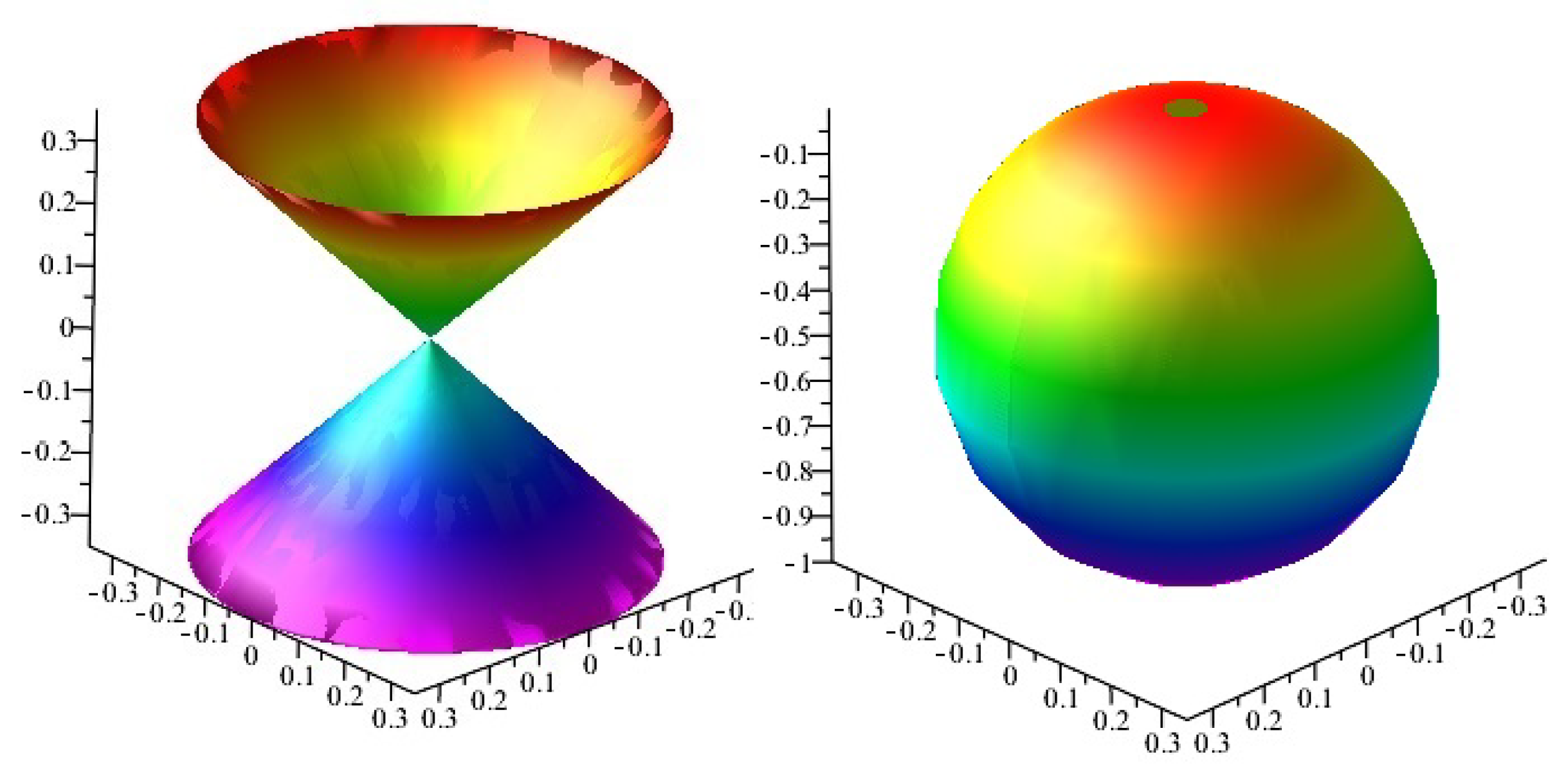
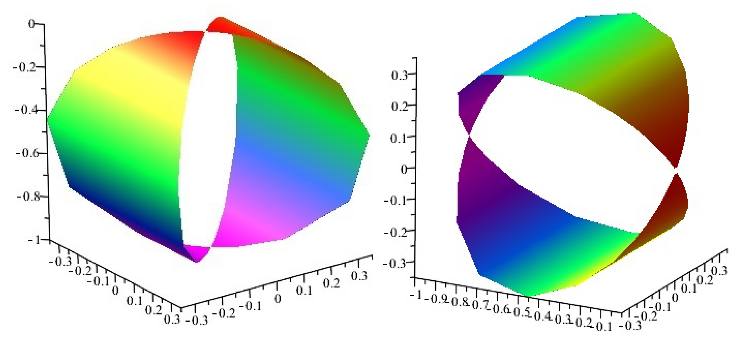
See Figure 1 and Figure 2 for some different projections and symmetries, from four-space to three-spaces of the Gauss map of the rotational hypersurface.

Thus, the shape operator of the rotational hypersurface is obtained as

$$\mathbf{S}=\left(\begin{array}{ccc}-\frac{{\phi }^{″}}{{\mathbf{W}}^3}& 0& 0\\ 0& -\frac{{\phi }^{\prime }}{u\mathbf{W}}& 0\\ 0& 0& -\frac{{\phi }^{\prime }}{u\mathbf{W}}\end{array}\right).$$

From these, we obtain the Gaussian curvature K and the mean curvature H of the rotational hypersurface as follows

$$K=-\frac{{\phi }^{\prime 2}{\phi }^{″}}{u^2{\mathbf{W}}^5}\mathrm{and}H=-\frac{u{\phi }^{″}+2{\phi }^{\prime 3}+2{\phi }^{\prime }}{3u{\mathbf{W}}^3}.$$

Therefore, we have the following corollaries:

Corollary 1.

Let $\mathbf{R}$ : $M^3$ ⟶ ${\mathbb{E}}^4$ be an isometric immersion given by (4). Then, $M^3$ has constant Gaussian curvature iff

$${\phi }^{\prime 4}{\phi }^{″2}-C{u}^4{(1+{\phi }^{\prime 2})}^5=0.$$

Corollary 2.

Let $\mathbf{R}$ : $M^3$ ⟶ ${\mathbb{E}}^4$ be an isometric immersion given by (4). Then, $M^3$ has constant mean curvature (CMC) iff

$${\left(u{\phi }^{\prime }+2{\phi }^{\prime 3}+2{\phi }^{\prime }\right)}^2-9C{u}^2{\left(1+{\phi }^{\prime 2}\right)}^3=0.$$

Corollary 3.

Let $\mathbf{R}$ : $M^3$ ⟶ ${\mathbb{E}}^4$ be an isometric immersion given by (4). Then, $M^3$ has zero Gaussian curvature iff

$$\phi \left(u\right)=c_{1}u+c_2,\mathrm{or}\phi \left(u\right)=c_1.$$

Proof. 

Solving the second order differential equation $K=0,$ i.e.,

$${\phi }^{\prime 2}{\phi }^{″}=0,$$

we get the solution.

Corollary 4.

Let $\mathbf{R}$ : $M^3$ ⟶ ${\mathbb{E}}^4$ be an isometric immersion given by (4). Then, $M^3$ has zero mean curvature iff

$$\phi \left(u\right)=\pm c_1\int \frac{du}{\sqrt{u^4-c_1}}+c_2.$$

Proof. 

When we solve the second order differential equation $H=0,$ i.e.,

$$u{\phi }^{″}+2{\phi }^{\prime 3}+2{\phi }^{\prime }=0,$$

we get the solution. Taking $z={\phi }^{\prime },$ $z^{\prime }={\phi }^{″}$, we have

$$\begin{array}{cc}\Rightarrow & u{z}^{\prime }+2z^3+2z=0\hfill \\ \Rightarrow & \frac{z^2{u}^4}{z^2+1}=c_1^2\hfill \\ \Rightarrow & \phi \left(u\right)=\pm c_1\int \frac{du}{\sqrt{u^4-c_1}}.\hfill \end{array}$$

Therefore, the solutions of $\phi \left(u\right)$ are given, by using Mathematica, as follows

$$\phi \left(u\right)=\pm \frac{i{c}_1\sqrt{\frac{1}{u^4-c_1}}\sqrt{1-\frac{u^4}{c_1}}\mathrm{EllipticF}\left[iargsinh\left[\sqrt{-\frac{1}{\sqrt{c_1}}}u\right],-1\right]}{\sqrt{-\frac{1}{\sqrt{c_1}}}}+c_2,$$

and, by using Maple, we get for the solutions $\phi \left(u\right)$:

$$\phi \left(u\right)=\pm \frac{c_1\sqrt{1+\frac{u^2}{\sqrt{c_1}}}\sqrt{1+\frac{u^2}{\sqrt{c_1}}}\mathrm{EllipticF}\left[u\sqrt{-\frac{1}{\sqrt{c_1}}}u,i\right]}{\sqrt{-\frac{1}{\sqrt{c_1}}}\sqrt{u^4-c_1}}+c_2,$$

where EllipticF[$\varphi$,m] gives the elliptic integral of the first kind F($\varphi \mid m$). □

Corollary 5.

Let $\mathbf{R}$ : $M^3$ ⟶ ${\mathbb{E}}^4$ be an isometric immersion given by 4. If $M^3$ has zero mean curvature, then we get

$$\phi \left(u\right)={\int }_1^{\infty }\frac{du}{\sqrt{u^4-1}}<\frac{\pi }{2},$$

where $u\in [1,\infty ).$

Proof. 

For the third kind improper integral ${\int }_1^{\infty }\frac{du}{\sqrt{u^4-1}},$ we get

$${\int }_1^{\infty }\frac{du}{\sqrt{u^4-1}}<{\int }_1^{\infty }\frac{du}{u\sqrt{u^2-1}}.$$

Taking $u=coshx,$ we have

$${\int }_1^{\infty }\frac{du}{u\sqrt{u^2-1}}={\int }_0^{\infty }\frac{dx}{coshx}=\frac{\pi }{2}.$$

□

4. Gauss Map

Next, we calculate the curvatures of the Gauss map (5) of the rotational hypersurface (4).

Theorem 2.

The Gaussian curvature and the mean curvature of the Gauss map (5) of the rotational hypersurface (4) are given as follows

$$K=-1andH=-1,$$

respectively,

Proof. 

Using the first partial differentials of (5), we get the first quantities as follows

$$\mathbf{I}=\left(\begin{array}{ccc}\frac{{\phi }^{″2}}{{\mathbf{W}}^4}& 0& 0\\ 0& \frac{{\phi }^{\prime 2}{cos}^{2}w}{{\mathbf{W}}^2}& 0\\ 0& 0& \frac{{\phi }^{\prime 2}}{{\mathbf{W}}^2}\end{array}\right).$$

We have

$$det\mathbf{I}=\frac{{\phi }^{\prime 4}{\phi }^{″2}{cos}^{2}w}{{\mathbf{W}}^8},$$

where $\phi =\phi \left(u\right),$ ${\phi }^{\prime }=\frac{d\phi }{du},$ ${\phi }^{″}=\frac{d^2\phi }{d{u}^2}.$ Using the second partial differentials of (5), we have the second quantities as follows

$$\mathbf{II}=\left(\begin{array}{ccc}-\frac{{\phi }^{″2}}{{\mathbf{W}}^4}& 0& 0\\ 0& -\frac{{\phi }^{\prime 2}{cos}^{2}w}{{\mathbf{W}}^2}& 0\\ 0& 0& -\frac{{\phi }^{\prime 2}}{{\mathbf{W}}^2}\end{array}\right),$$

where

$$det\mathbf{II}=-\frac{{\phi }^{\prime 4}{\phi }^{″2}{cos}^{2}w}{{\mathbf{W}}^8}.$$

The Gauss map of the Gauss map (5) of the rotational hypersurface (4） is

$${\mathbf{e}}_{\left({\mathbf{e}}_{{}_{\mathbf{R}}}\right)}=\frac{1}{\mathbf{W}}\left(\begin{array}{c}{\phi }^{\prime }cosvcosw\\ {\phi }^{\prime }sinvcosw\\ {\phi }^{\prime }sinw\\ -1\end{array}\right).$$

(6)

The shape operator of （6） is

$$\mathbf{S}=\left(\begin{array}{ccc}-1& 0& 0\\ 0& -1& 0\\ 0& 0& -1\end{array}\right).$$

Finally, we obtain the Gaussian curvature and the mean curvature of （5） as $K=-1,$ and $H=-1.$ □

5. The Third Laplace–Beltrami Operator

Next, we introduce the third Laplace–Beltrami operator to the four-space. Then, we apply it for the hypersurface (4). See [28] for the Laplace–Beltrami operator in three-space.

The inverse of the matrix

$$\left(e_{ij}\right)=\left(\begin{array}{ccc}{e}_{11}& e_{12}& e_{13}\\ e_{21}& e_{22}& e_{23}\\ e_{31}& e_{32}& e_{33}\end{array}\right)$$

is as follows

$$\frac{1}{e}\left(\begin{array}{ccc}{e}_{22}{e}_{33}-e_{23}{e}_{32}& -\left(e_{12}{e}_{33}-e_{13}{e}_{32}\right)& e_{12}{e}_{23}-e_{13}{e}_{22}\\ -\left(e_{21}{e}_{33}-e_{31}{e}_{23}\right)& e_{11}{e}_{33}-e_{13}{e}_{31}& -\left(e_{11}{e}_{23}-e_{21}{e}_{13}\right)\\ e_{21}{e}_{32}-e_{22}{e}_{31}& -\left(e_{11}{e}_{32}-e_{12}{e}_{31}\right)& e_{11}{e}_{22}-e_{12}{e}_{21}\end{array}\right),$$

where

$$\begin{array}{ccc}\hfill e& =& det\left(e_{ij}\right)\hfill \\ & =& e_{11}{e}_{22}{e}_{33}-e_{11}{e}_{23}{e}_{32}+e_{12}{e}_{31}{e}_{23}-e_{12}{e}_{21}{e}_{33}+e_{21}{e}_{13}{e}_{32}-e_{13}{e}_{22}{e}_{31}.\hfill \end{array}$$

Definition 2.

The third Laplace–Beltrami operator ${\Delta }^{\mathbf{III}}$ of hypersurface $\mathbf{M}$ is as follows

$${\Delta }^{\mathbf{III}}\varphi =\frac{1}{\sqrt{e}}\sum _{i,j=1}^3\frac{\partial }{\partial x^i}\left(\sqrt{e}{e}^{ij}\frac{\partial \varphi }{\partial x^j}\right),$$

(7)

where $\left(e^{ij}\right)={\left(e_{kl}\right)}^{-1}$ and $e=det\left(e_{ij}\right)$ and $\varphi =\varphi (x^1,x^2,x^3){\mid }_{\mathbf{D}}$ $(\mathbf{D}\subset {\mathbb{R}}^3)$ is a smooth function of class $C^3$. We can write ${\Delta }^{\mathbf{III}}\varphi$ as follows

$$\frac{1}{\sqrt{e}}\left[\begin{array}{c}\frac{\partial }{\partial x^1}\left(\sqrt{e}{e}^{11}\frac{\partial \varphi }{\partial x^1}\right)-\frac{\partial }{\partial x^1}\left(\sqrt{e}{e}^{12}\frac{\partial \varphi }{\partial x^2}\right)+\frac{\partial }{\partial x^1}\left(\sqrt{e}{e}^{13}\frac{\partial \varphi }{\partial x^3}\right)\\ -\frac{\partial }{\partial x^2}\left(\sqrt{e}{e}^{21}\frac{\partial \varphi }{\partial x^1}\right)+\frac{\partial }{\partial x^2}\left(\sqrt{e}{e}^{22}\frac{\partial \varphi }{\partial x^2}\right)-\frac{\partial }{\partial x^2}\left(\sqrt{e}{e}^{23}\frac{\partial \varphi }{\partial x^3}\right)\\ +\frac{\partial }{\partial x^3}\left(\sqrt{e}{e}^{31}\frac{\partial \varphi }{\partial x^1}\right)-\frac{\partial }{\partial x^3}\left(\sqrt{e}{e}^{32}\frac{\partial \varphi }{\partial x^2}\right)+\frac{\partial }{\partial x^3}\left(\sqrt{e}{e}^{33}\frac{\partial \varphi }{\partial x^3}\right)\end{array}\right].$$

Clearly, we can write the matrix of the third fundamental form

$$\mathbf{III}=\left(\begin{array}{ccc}X& Y& U\\ Y& Z& J\\ U& J& O\end{array}\right),$$

(8)

where

$$\begin{array}{ccc}\hfill X& =& {\mathbf{e}}_u·{\mathbf{e}}_u,Y={\mathbf{e}}_u·{\mathbf{e}}_v,U={\mathbf{e}}_u·{\mathbf{e}}_w,\hfill \\ \hfill Z& =& {\mathbf{e}}_v·{\mathbf{e}}_v,J={\mathbf{e}}_v·{\mathbf{e}}_w,O={\mathbf{e}}_w·{\mathbf{e}}_w.\hfill \end{array}$$

Here, $\mathbf{e}$ is the Gauss map (i.e., the unit normal vector). More precisely, we get

$${\mathbf{III}}^{-1}=\frac{1}{det\mathbf{III}}\left(\begin{array}{ccc}OZ-J^2& JU-OY& JY-UZ\\ JU-OY& OX-U^2& UY-JX\\ JY-UZ& UY-JX& XZ-Y^2\end{array}\right),$$

where

$$det\mathbf{III}=\left(XZ-Y^2\right)O-J^{2}X+2JUY-U^{2}Z.$$

Hence, using a function $\varphi =\varphi (u,v,w)$, we specifically obtain

$${\Delta }^{\mathbf{III}}\varphi =\frac{1}{\sqrt{\left|det\mathbf{III}\right|}}\left[\begin{array}{c}\frac{\partial }{\partial u}\left(\frac{\left(OZ-J^2\right){\varphi }_u-\left(JU-OY\right){\varphi }_v+\left(JY-UZ\right){\varphi }_w}{\sqrt{\left|det\mathbf{III}\right|}}\right)\\ -\frac{\partial }{\partial v}\left(\frac{\left(JU-OY\right){\varphi }_u-\left(OX-U^2\right){\varphi }_v+\left(UY-JX\right){\varphi }_w}{\sqrt{\left|det\mathbf{III}\right|}}\right)\\ +\frac{\partial }{\partial w}\left(\frac{\left(JY-UZ\right){\varphi }_u-\left(UY-JX\right){\varphi }_v+\left(XZ-Y^2\right){\varphi }_w}{\sqrt{\left|det\mathbf{III}\right|}}\right)\end{array}\right].$$

(9)

We continue our calculations to find the third Laplace–Beltrami operator ${\Delta }^{\mathbf{III}}\mathbf{R}$ of the rotational hypersurface $\mathbf{R}$ using (9) in (4).

The third Laplace–Beltrami operator of the hypersurface parametrized by (4) is given by

$${\Delta }^{\mathbf{III}}\mathbf{R}=\frac{1}{\sqrt{\left|det\mathbf{III}\right|}}\left(\frac{\partial }{\partial u}\mathbf{U}-\frac{\partial }{\partial v}\mathbf{V}+\frac{\partial }{\partial w}\mathbf{W}\right),$$

where

$$\begin{array}{ccc}\hfill \mathbf{U}& =& \frac{\left(OZ-J^2\right){\mathbf{R}}_u-\left(JU-OY\right){\mathbf{R}}_v+\left(JY-UZ\right){\mathbf{R}}_w}{\sqrt{\left|det\mathbf{III}\right|}},\hfill \\ \hfill \mathbf{V}& =& \frac{\left(JU-OY\right){\mathbf{R}}_u-\left(OX-U^2\right){\mathbf{R}}_v+\left(UY-JX\right){\mathbf{R}}_w}{\sqrt{\left|det\mathbf{III}\right|}},\hfill \\ \hfill \mathbf{W}& =& \frac{\left(JY-UZ\right){\mathbf{R}}_u-\left(UY-JX\right){\mathbf{R}}_v+\left(XZ-Y^2\right){\mathbf{R}}_w}{\sqrt{\left|det\mathbf{III}\right|}}.\hfill \end{array}$$

Here, using the parametrization $,$ we get $Y=U=J=0.$ Therefore, we have the following

$$\mathbf{U}=\frac{OZ}{\sqrt{\left|det\mathbf{III}\right|}}{\mathbf{R}}_u=\left(\frac{{\phi }^{\prime 4}{cos}^{2}w}{{\left(1+{\phi }^{\prime 2}\right)}^2\sqrt{\left|det\mathbf{III}\right|}}\right){\mathbf{R}}_u,$$

$$\mathbf{V}=-\frac{OX}{\sqrt{\left|det\mathbf{III}\right|}}{\mathbf{R}}_v=\left(-\frac{{\phi }^{\prime 2}{\phi }^{\prime \prime 2}}{{\left(1+{\phi }^{\prime 2}\right)}^3\sqrt{\left|det\mathbf{III}\right|}}\right){\mathbf{R}}_v,$$

$$\mathbf{W}=\frac{XZ}{\sqrt{\left|det\mathbf{III}\right|}}{\mathbf{R}}_w=\left(\frac{{\phi }^{\prime 2}{\phi }^{\prime \prime 2}{cos}^{2}w}{{\left(1+{\phi }^{\prime 2}\right)}^3\sqrt{\left|det\mathbf{III}\right|}}\right){\mathbf{R}}_w,$$

where

$$det\mathbf{III}=\frac{{\phi }^{\prime 4}{\phi }^{″2}{cos}^{2}w}{{(1+{\phi }^{\prime 2})}^4}.$$

We obtain the vectors

$$\mathbf{U}=\frac{{\phi }^{\prime 2}cosw}{{\left(1+{\phi }^{\prime 2}\right)}^2{\phi }^{″}}\left(\begin{array}{c}cosvcosw\\ sinvcosw\\ sinw\\ {\phi }^{\prime }\end{array}\right),$$

$$\mathbf{V}=-\frac{{\phi }^{″}}{\left(1+{\phi }^{\prime 2}\right)cosw}\left(\begin{array}{c}-usinvcosw\\ ucosvcosw\\ 0\\ 0\end{array}\right)$$

and

$$\mathbf{W}=\frac{{\phi }^{″}cosw}{1+{\phi }^{\prime 2}}\left(\begin{array}{c}-ucosvsinw\\ -usinvsinw\\ ucosw\\ 0\end{array}\right).$$

Taking differentials with respect to $u,v$ and w on $\mathbf{U},\mathbf{V},\mathbf{W},$ respectively, we get

$$\frac{\partial }{\partial u}\left(\mathbf{U}\right)=\frac{\partial }{\partial u}\left(\frac{{\phi }^{\prime 2}}{{\left(1+{\phi }^{\prime 2}\right)}^2{\phi }^{″}}\right)\left(\begin{array}{c}cosv{cos}^{2}w\\ sinv{cos}^{2}w\\ sinvcosw\\ {\phi }^{\prime }cosw\end{array}\right)+\frac{{\phi }^{\prime 2}}{{\left(1+{\phi }^{\prime 2}\right)}^2}\left(\begin{array}{c}0\\ 0\\ 0\\ cosw\end{array}\right),$$

$$\frac{\partial }{\partial v}\left(\mathbf{V}\right)=-\frac{{\phi }^{″}}{\left(1+{\phi }^{\prime 2}\right)}\left(\begin{array}{c}-ucosv\\ -usinv\\ 0\\ 0\end{array}\right),$$

$$\frac{\partial }{\partial w}\left(\mathbf{W}\right)=\frac{{\phi }^{″}}{1+{\phi }^{\prime 2}}\left(\begin{array}{c}ucosvcos2w\\ usinvcos2w\\ -usin2w\\ 0\end{array}\right).$$

Therefore, we obtain the following theorem:

Theorem 3.

The third Laplace–Beltrami operator of the hypersurface (4) is given by

$$\begin{array}{ccc}\hfill {\Delta }^{\mathbf{III}}{\mathbf{R}}_1& =& \eta .\{[-4{\phi }^{\prime }{\phi }^{″}+2{\phi }^{\prime }\left(1+{\phi }^{\prime 2}\right){\phi }^{″2}-\left(1+{\phi }^{\prime 2}\right){\phi }^{‴}]cosv{cos}^{2}w\hfill \\ & & +\left(1+{\phi }^{\prime 2}\right)ucosv{\phi }^{″3}+\left(1+{\phi }^{\prime 2}\right)ucosvcos2w{\phi }^{″3}\},\hfill \end{array}$$

$$\begin{array}{ccc}\hfill {\Delta }^{\mathbf{III}}{\mathbf{R}}_2& =& \eta .\{[-4{\phi }^{\prime }{\phi }^{″}+2{\phi }^{\prime }\left(1+{\phi }^{\prime 2}\right){\phi }^{″2}-\left(1+{\phi }^{\prime 2}\right){\phi }^{‴}]sinv{cos}^{2}w\hfill \\ & & +\left(1+{\phi }^{\prime 2}\right)usinv{\phi }^{″3}+\left(1+{\phi }^{\prime 2}\right)usinvcos2w{\phi }^{″3}\},\hfill \end{array}$$

$$\begin{array}{ccc}\hfill {\Delta }^{\mathbf{III}}{\mathbf{R}}_3& =& \eta .\{[-4{\phi }^{\prime }{\phi }^{″}+2{\phi }^{\prime }\left(1+{\phi }^{\prime 2}\right){\phi }^{″2}-\left(1+{\phi }^{\prime 2}\right){\phi }^{‴}]sinvcosw\hfill \\ & & -\left(1+{\phi }^{\prime 2}\right)usin2w{\phi }^{″3}\},\hfill \end{array}$$

$$\begin{array}{ccc}\hfill {\Delta }^{\mathbf{III}}{\mathbf{R}}_4& =& \eta .\{[-4{\phi }^{\prime }{\phi }^{″}+2{\phi }^{\prime }\left(1+{\phi }^{\prime 2}\right){\phi }^{″2}-\left(1+{\phi }^{\prime 2}\right){\phi }^{‴}]cosw{\phi }^{\prime }\hfill \\ & & +cosw{\phi }^{\prime 2}{\phi }^{″2}\},\hfill \end{array}$$

where

$${\Delta }^{\mathbf{III}}\mathbf{R}=\left({\Delta }^{\mathbf{III}}{\mathbf{R}}_1,{\Delta }^{\mathbf{III}}{\mathbf{R}}_2,{\Delta }^{\mathbf{III}}{\mathbf{R}}_3,{\Delta }^{\mathbf{III}}{\mathbf{R}}_4\right),$$

and

$$\eta =\eta (u,w)={\left({\phi }^{\prime 2}{\phi }^{″3}cosw\right)}^{-1}.$$

6. Conclusions

When the rotational hypersurface $\mathbf{R}$ has the equation ${\Delta }^{\mathbf{III}}\mathbf{R}=\mathbf{0},$ i.e., the rotational hypersurface （4) is $\mathbf{III}$-minimal, then we have to solve the system of equation

$${\Delta }^{\mathbf{III}}{\mathbf{R}}_i=0,$$

where $1\le i\le 4$. In fact, the $\mathbf{III}$-minimal hypersurface of the four-space is a very interesting problem. It is challenging to solve the above equations.

When $\phi \ne c=const.$ or $\phi \ne c_{1}u+c_2,$ and ${\theta }_2\ne \frac{\pi }{2}+2k\pi ,$ $k\in \mathbb{Z},$ we get ${\Delta }^{\mathbf{III}}\mathbf{R}\ne \mathbf{0}.$ Hence, the rotational hypersurface (4) is not $\mathbf{III}$-minimal.

References

- Arslan, K.; Deszcz, R.; Yaprak, Ş. On Weyl pseudosymmetric hypersurfaces. Colloq. Math. 1997, 72, 353–361. [Google Scholar] [CrossRef]
- Arslan, K.; Kılıç Bayram, B.; Bulca, B.; Öztürk, G. Generalized Rotation Surfaces in . Results Math. 2012, 61, 315–327. [Google Scholar] [CrossRef]
- Arvanitoyeorgos, A.; Kaimakamis, G.; Magid, M. Lorentz hypersurfaces in satisfying ΔH = αH. Ill. J. Math. 2009, 53, 581–590. [Google Scholar]
- Chen, B.Y. Total Mean Curvature and Submanifolds of Finite Type; World Scientific: Singapore, 1984. [Google Scholar]
- Chen, B.Y.; Choi, M.; Kim, Y.H. Surfaces of revolution with pointwise 1-type Gauss map. Korean Math. Soc. 2005, 42, 447–455. [Google Scholar] [CrossRef]
- Dursun, U.; Turgay, N.C. Minimal and pseudo-umbilical rotational surfaces in Euclidean space . Mediterr. J. Math. 2013, 10, 497–506. [Google Scholar] [CrossRef]
- Kim, Y.H.; Turgay, N.C. Surfaces in with L1-pointwise 1-type Gauss map. Bull. Korean Math. Soc. 2013, 50, 935–949. [Google Scholar] [CrossRef]
- Takahashi, T. Minimal immersions of Riemannian manifolds. J. Math. Soc. Jpn. 1966, 18, 380–385. [Google Scholar] [CrossRef]
- Magid, M.; Scharlach, C.; Vrancken, L. Affine umbilical surfaces in . Manuscr. Math. 1995, 88, 275–289. [Google Scholar] [CrossRef]
- Vlachos, T. Hypersurfaces in with harmonic mean curvature vector field. Math. Nachr. 1995, 172, 145–169. [Google Scholar]
- Scharlach, C. Affine Geometry of Surfaces and Hypersurfaces in . In Symposium on the Differential Geometry of Submanifolds; Dillen, F., Simon, U., Vrancken, L., Eds.; Un. Valenciennes: Valenciennes, France, 2007; Volume 124, pp. 251–256. [Google Scholar]
- Cheng, Q.M.; Wan, Q.R. Complete hypersurfaces of with constant mean curvature. Monatsh. Math. 1994, 118, 171–204. [Google Scholar] [CrossRef]
- Moore, C. Surfaces of rotation in a space of four dimensions. Ann. Math. 1919, 21, 81–93. [Google Scholar] [CrossRef]
- Moore, C. Rotation surfaces of constant curvature in space of four dimensions. Bull. Am. Math. Soc. 1920, 26, 454–460. [Google Scholar] [CrossRef]
- Ganchev, G.; Milousheva, V. General rotational surfaces in the 4-dimensional Minkowski space. Turk. J. Math. 2014, 38, 883–895. [Google Scholar] [CrossRef] [Green Version]
- Dillen, F.; Fastenakels, J.; Van der Veken, J. Rotation hypersurfaces of and . Note Mat. 2009, 29-1, 41–54. [Google Scholar]
- Senoussi, B.; Bekkar, M. Helicoidal surfaces with ΔJr = Ar in 3-dimensional Euclidean space. Stud. Univ. Babeş-Bolyai Math. 2015, 60, 437–448. [Google Scholar]
- Bour, E. Théorie de la déformation des surfaces. J. Êcole Imp. Polytech. 1862, 22, 1–148. [Google Scholar]
- Do Carmo, M.; Dajczer, M. Helicoidal surfaces with constant mean curvature. Tohoku Math. J. 1982, 34, 351–367. [Google Scholar] [CrossRef]
- Güler, E. Bour’s theorem and light-like profile curve. Yokohama Math. J. 2007, 54, 155–157. [Google Scholar]
- Hieu, D.T.; Thang, N.N. Bour’s theorem in 4-dimensional Euclidean space. Bull. Korean Math. Soc. 2017, 54, 2081–2089. [Google Scholar]
- Choi, M.; Kim, Y.H.; Liu, H.; Yoon, D.W. Helicoidal surfaces and their Gauss map in Minkowski 3-space. Bull. Korean Math. Soc. 2010, 47, 859–881. [Google Scholar] [CrossRef]
- Choi, M.; Kim, Y.H. Characterization of the helicoid as ruled surfaces with pointwise 1-type Gauss map. Bull. Korean Math. Soc. 2001, 38, 753–761. [Google Scholar]
- Choi, M.; Yoon, D.W. Helicoidal surfaces of the third fundamental form in Minkowski 3-space. Bull. Korean Math. Soc. 2015, 52, 1569–1578. [Google Scholar] [CrossRef]
- Ferrandez, A.; Garay, O.J.; Lucas, P. On a Certain Class of Conformally at Euclidean Hypersurfaces. In Global Analysis and Global Differential Geometry; Springer: Berlin, Germany, 1990; pp. 48–54. [Google Scholar]
- Verstraelen, L.; Valrave, J.; Yaprak, Ş. The minimal translation surfaces in Euclidean space. Soochow J. Math. 1994, 20, 77–82. [Google Scholar]
- Güler, E.; Magid, M.; Yaylı, Y. Laplace Beltrami operator of a helicoidal hypersurface in four space. J. Geom. Symmetry Phys. 2016, 41, 77–95. [Google Scholar]
- Lawson, H.B. Lectures on Minimal Submanifolds, 2nd ed.; Mathematics Lecture Series 9; Publish or Perish, Inc.: Wilmington, Delaware, 1980. [Google Scholar]
Figure 1.
Projections of : (left) into -space; (right) into -space;
Figure 2.
© 2018 by the authors. Licensee MDPI, Basel, Switzerland. This article is an open access article distributed under the terms and conditions of the Creative Commons Attribution (CC BY) license (http://creativecommons.org/licenses/by/4.0/).
Share and Cite
MDPI and ACS Style
Güler, E.; Hacısalihoğlu, H.H.; Kim, Y.H. The Gauss Map and the Third Laplace-Beltrami Operator of the Rotational Hypersurface in 4-Space. Symmetry 2018, 10, 398. https://doi.org/10.3390/sym10090398
AMA Style
Güler E, Hacısalihoğlu HH, Kim YH. The Gauss Map and the Third Laplace-Beltrami Operator of the Rotational Hypersurface in 4-Space. Symmetry. 2018; 10(9):398. https://doi.org/10.3390/sym10090398
Chicago/Turabian StyleGüler, Erhan, Hasan Hilmi Hacısalihoğlu, and Young Ho Kim. 2018. "The Gauss Map and the Third Laplace-Beltrami Operator of the Rotational Hypersurface in 4-Space" Symmetry 10, no. 9: 398. https://doi.org/10.3390/sym10090398
Note that from the first issue of 2016, this journal uses article numbers instead of page numbers. See further details here.